Abstract
Electromagnetic (EM) surveys play a significant role in mineral exploration. However, the EM method often faces limitations when investigating minerals in areas covered by rivers, lakes, or other water bodies. This paper introduces audio magnetotelluric (AMT) observation technology that utilizes separated electric and magnetic channels to deal with this challenge over water-covered areas. The study analyzes and discusses the characteristics of the relative error of the magnetic field through forward simulation. The observation and profile experiments were conducted at the estuary of a river in Liaoning Province, China, and high-quality data in the river and the pseudo-geoelectric section of the underwater space were successfully obtained. The results demonstrate the feasibility and effectiveness of the AMT observation technology over water-covered areas, emphasizing the importance of locating the magnetic channel in a quiet zone at a certain distance from the shore. This configuration helps reduce the influence of resistivity differences between water and shore, ultimately improving data quality and accuracy. The research suggests that the AMT observation technology, utilizing separated electric and magnetic channels, has the potential for further improvement and can serve as a valuable guide for mineral exploration over water-covered areas.
1. Introduction
In modern times, the growing demand for various mineral resources has led to the development of numerous geophysical technologies and equipment, significantly enhancing their ability to explore mineral deposits beneath complex covers. Among these techniques, the electromagnetic (EM) method stands out as a popular geophysical exploration tool. It has several excellent characteristics, including low cost, high work efficiency, great detection depth, and minimal susceptibility to terrain effects. Consequently, it has found extensive application in the surveying of mineral resources, engineering exploration, and environmental monitoring worldwide [1,2]. However, the EM method often faces challenges in detecting and discovering mineral deposits over water-covered areas, such as brine resources in or under salt lakes [3] and lithium–boron deposits and potassium deposits under large salt lakes [4,5]. Therefore, the development of effective EM technologies for mineral exploration over water-covered areas can be significant and useful.
Magnetotelluric (MT) sounding is the primary EM method used for marine surveys [6]. The initial applications of MT sounding in shallow seas were discussed by Filloux (1973), Bennett and Filloux (1975), Filloux (1980), and Chave and Filloux (1984) [7,8,9,10]. Since the beginning of this century, marine frequency-domain EM methods have experienced rapid development [11,12,13,14]. While Chinese geophysicists entered this field relatively late, they have conducted numerous studies and have found several applications [15,16,17,18,19,20,21]. However, exploration technologies in deep water have challenging requirements on equipment and result in high costs.
Due to the limitations of geophysical equipment, land-based EM methods are generally unsuitable for mineral resource surveying and engineering exploration over water-covered areas. Consequently, limited research and applications have been reported in this domain. Various techniques such as water-based resistivity surveying, electrical resistivity tomography (ERT), continuous resistivity profiling, and the transient electromagnetic method (TEM) have been proposed and applied for investigations related to groundwater discharge, rock tunnels, and sediments beneath lakes [22,23,24,25]. ERT and audio magnetotelluric (AMT) sounding have shown promising application results in hydrothermal systems under volcanic lakes [26,27]. In China, MT surveys have primarily focused on shallow seas [15,28,29,30,31], while other methods have been employed for underground exploration in rivers and lakes. The spectrum-induced polarization method was used for geological surveying beneath a river [32]; the high-density resistivity method was applied in the construction of a cross-river tunnel and oil pipelines [33,34]; and TEM was the most commonly used EM method for geological surveying beneath rivers [35,36,37,38].
AMT sounding, known for its natural field source and large exploration depth, has found widespread application in geological and mineral explorations [39,40,41]. However, when land-based AMT equipment is used for underwater exploration in rivers and lakes, the magnetic sensor is prone to damage due to its poor waterproof performance. Additionally, accurately fixing the magnetic sensor in a specific horizontal direction over the water poses another challenge. Typically, AMT surveys in an aquatic environment are conducted by placing the magnetic channel on the shore and the electric channel over the water or on the water body floor, with synchronous recording of magnetic and electric fields [30,42].
Moreover, setting up channels on the water body floor is complicated due to the invisible topography of the water floor. Another challenge arises from the electric field differences between the surface and the water floor caused by the overlying water layer. The electric field needs to be corrected to the plane where the sensor is located [29,30]. To address these issues, this research applied an AMT observation technology of separated electric and magnetic channels over water-covered areas. The electric channel was positioned over the water, while the magnetic channel was placed on the shore to simultaneously measure the electric and magnetic fields.
The key precondition for this study is whether the magnetic field on the shore can replace the magnetic field over the water. In homogeneous media or horizontally layered media, when the initial incident wave is a plane EM wave, the horizontal component of the total magnetic field on the ground is always twice that of the primary magnetic field, regardless of the variation in the underground resistivity [43]. Therefore, the magnetic field on the ground does not carry any electrical information about the underground media, and only the horizontal component of the electric field is related to the underground geoelectric section. In the early 1970s, the telluric–magnetotelluric method used the magnetic field at the base site as the magnetic field for the whole work area, with telluric field measurements taken only at remote sites. This approach yielded successful results in beaches and geothermal explorations [44,45]. Ding (2006), Yang (2006), and Xu (2006) conducted MT observation experiments using separated electric and magnetic channels on beaches and discussed the influence of the water layer on the magnetic field [29,30,31]. However, for inhomogeneous media, when the AMT survey takes the magnetic field at the base site as the magnetic field for the whole work area, it may introduce errors and reduce exploration accuracy.
In this study, we introduced an AMT observation technology using separated electric and magnetic channels over water-covered areas. This approach involves synchronously measuring the electric field over the water and the magnetic field on the shore. Through forward modeling, we initially analyzed the distribution characteristics of magnetic field errors caused by separated electric and magnetic channels and discussed methods to mitigate these influences. Subsequently, we conducted observation and profile experiments using separated electric and magnetic channels at the estuary of a river in Liaoning Province, China. The results confirm the feasibility of the AMT observation technology proposed in this study, providing guidance for EM surveys over water-covered areas.
2. Technology of Separated Electric and Magnetic Channels
The magnetotelluric equation [6] is expressed as follows:
where E and H represent the electric and magnetic fields, respectively, while Z denotes the impedance tensor. At the measuring point (i.e., electric channel site) P, we define EP and HP as the electric and magnetic fields, respectively. Additionally, we designate HM as the magnetic field at the magnetic channel site. Under the separated electric and magnetic channels mode, if the magnetic field of the magnetic channel site HM replaces the magnetic field of the measuring point HP, the impedance tensor of the measuring point P (ZPM) can be represented as
Furthermore, the relative error of the magnetic field caused by the separated electric and magnetic channels is given by
3. Numerical Simulation of Separated Electric and Magnetic Channels
To quantitatively analyze the variation characteristics of the horizontal component of the magnetic field under the separated electric and magnetic channels mode, we employed the two-dimensional (2D) AMT finite-element method [46] for numerical simulation. The forward modeling involved the inhomogeneous geoelectric model and the water body model. We conducted respective simulations for each and analyzed the relative errors of the horizontal component of the magnetic field resulting from the separated electric and magnetic channels. The frequency range used for forward modeling was 0.35–10,400 Hz. In 2D cases, as the geological body is infinite along the strike direction, the magnetic field component in the horizontal direction remains constant. Therefore, we focus on discussing the horizontal component of the magnetic field in the dip direction of the geological body only.
3.1. Inhomogeneous Geoelectric Model
As shown in Figure 1, the underground medium consists of two different geoelectric units, with the interface located at the center of the profile (0, 0). The left geoelectric body has a lower resistivity of 50 Ω∙m, while the resistivity of the right geoelectric body is higher. To examine the influence of resistivity differences on the magnetic field, we set the resistivities of the right geoelectric body to 200/500/2000 Ω∙m, respectively. Through AMT forward modeling, we computed the changes in the magnetic field along the profile and the relative errors under the separated electric and magnetic channels mode. The results are presented in Figure 2, Figure 3, Figure 4 and Figure 5.
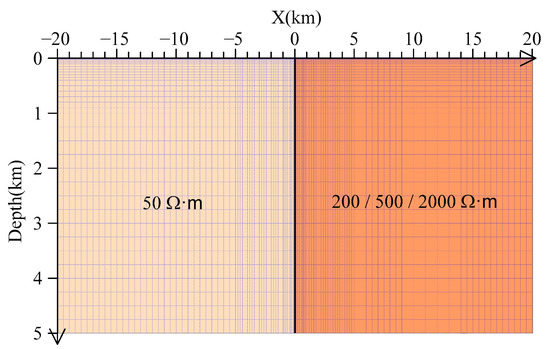
Figure 1.
Sketch map of the inhomogeneous geoelectric model. The blue lines represent the forward mesh.
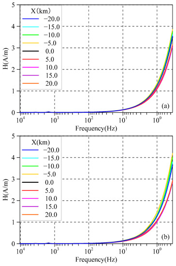
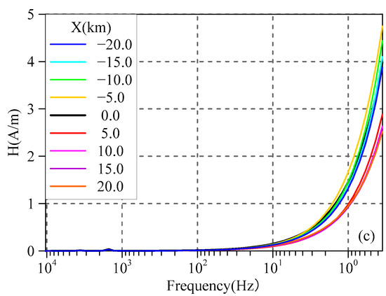
Figure 2.
Comparison of the magnetic field at different positions along the profile of the inhomogeneous geoelectric model with the right geoelectric body’s resistivity of (a) 200 Ω∙m, (b) 500 Ω∙m, and (c) 2000 Ω∙m.
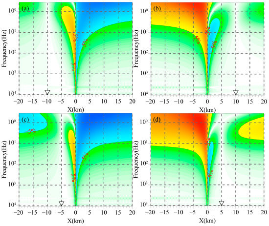
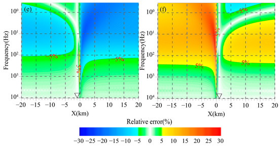
Figure 3.
Contour maps of the relative error of the magnetic field at different positions along the profile of the inhomogeneous geoelectric model with the right geoelectric body’s resistivity set at 200 Ω∙m. The measuring points are at (a) −10.0 km, (b) 10.0 km, (c) −5.0 km, (d) 5.0 km, (e) −1.0 km, and (f) 1.0 km. The inverted triangle indicates the location of the measuring point.
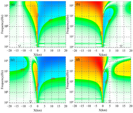
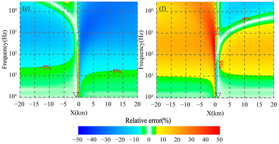
Figure 4.
Contour maps of the relative error of the magnetic field at different positions along the profile of the inhomogeneous geoelectric model with the right geoelectric body’s resistivity set at 500 Ω∙m. The measuring points are at (a) −13.0 km, (b) 13.0 km, (c) −5.0 km, (d) 5.0 km, (e) −1.0 km, and (f) 1.0 km. The inverted triangle indicates the location of the measuring point.
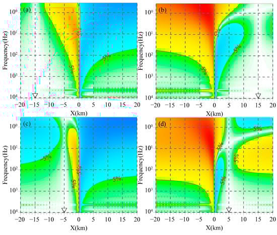
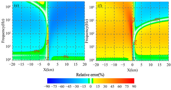
Figure 5.
Contour maps of the relative error of the magnetic field at different positions on the profile of the inhomogeneous geoelectric model with the right geoelectric body’s resistivity set at 2000 Ω∙m. The measuring points are at (a) −15.0 km, (b) 15.0 km, (c) −5.0 km, (d) 5.0 km, (e) −1.0 km, and (f) 1.0 km. The inverted triangle indicates the location of the measuring point.
As Figure 2 shows, the magnetic fields of different geoelectric bodies on the profile increase with the decrease in frequency. The curves exhibit good agreement in the frequency range of 10–10,400 Hz, but gradually diverge at lower frequencies from approximately 10 Hz, with the differences becoming more pronounced as the frequency decreases. In high-resistivity regions, the magnetic field on the profile is lower than that at the interface, while it is the opposite in low-resistivity regions. Comparing Figure 2a–c, it can be seen that the greater the electrical difference between the media on two sides of the interface, the larger the magnetic field difference on the profile at lower frequencies.
Figure 3, Figure 4 and Figure 5 illustrate the distribution of the relative error of the magnetic field with the frequency caused by replacing the magnetic field at the measuring point with that of the magnetic channel at different positions along the profile. In this study, we take 5% as the threshold value of the relative error, irrespective of its positive or negative sign. It can be seen from Figure 3, Figure 4 and Figure 5 that the relative errors of the magnetic field caused by electrical differences of geoelectric bodies are primarily concentrated in the middle-low frequency band and are distributed on both sides of the interface. When the magnetic channel and the measuring point are in the same geoelectric unit, the influence of electrical difference on the magnetic field becomes more complex. Specifically, between the measuring point and the interface, the relative error of the magnetic field exceeding 5% is primarily observed in the middle-low frequency band. As the magnetic channel approaches the interface, the effect gradually extends to the high-frequency band. On the opposite side of the measuring point, the relative error of the magnetic field is mainly concentrated in the low-frequency band. As the magnetic channel gradually moves away from the measuring point, the effect also extends to the high-frequency band. When the magnetic channel and the measuring point are in different geoelectric units, the relative error of the magnetic field consistently exceeds 5% in the low-frequency band, and the magnitude of the error increases as the frequency decreases. As the magnetic channel approaches the interface, the effect gradually extends to the high-frequency band. Comparing Figure 3a,c,e, it can be observed that as the measuring point approaches the interface, the frequency band where the relative error of the magnetic field exceeds 5% gradually expands from the low to high frequencies, which aligns with the frequency band in Figure 3b,d,f.
Comparing Figure 3, Figure 4 and Figure 5 reveals that the greater the electrical difference between the two sides of the interface, the larger the relative error range of the magnetic field. Specifically, as shown in Figure 3a,b, when the measuring point is 10 km away from the interface, the relative error of the magnetic field in the area over 5.0 km away from the interface on the same side remains below 5%. Similarly, as shown in Figure 4a,b, when the measuring point is 13.0 km away from the interface, the relative error of the magnetic field in the area over 8.0 km away from the interface on the same side stays below 5%. Furthermore, as shown in Figure 5a,b, when the measuring point is 15.0 km away from the interface, the relative error of the magnetic field in the area over 12.0 km away from the interface on the same side remains below 5%.
Based on the above analysis, it is evident that under the separated electric and magnetic channels mode, the influence of inhomogeneous geoelectric units on the magnetic field is relatively complex. In the same geoelectric unit, the influence is primarily concentrated near the interface. However, in different geoelectric units, the low-frequency magnetic field in all regions is consistently affected. Therefore, under the separated electric and magnetic channels mode, it is recommended to position the magnetic channel in the same geoelectric unit as the measuring point, with a certain distance from the interface. This distance should increase with the increase in the electrical difference between the geological units on two sides of the interface, and it is preferable to focus on observing the high-frequency band.
3.2. Water Body Model
In China, inland rivers, lakes, and other water bodies are typically situated on sedimentary strata or bedrock, with the resistivity of the water bodies generally being n × 101–102 Ω∙m within tens of meters. The sedimentary strata consist of clay (10−1–101 Ω∙m), mudstone (101–102 Ω∙m), siltstone (101–102 Ω∙m), and sandstone (101–103 Ω∙m). The bedrock tends to have higher resistivity, approximately n × (102–103) Ω∙m. Consequently, we established two water models. As depicted in Figure 6, the water is located at the center of the land (0, 0), with a width of 1000 m. The water depth increases from the shore to the center over a distance of 20 m, and the water resistivity is 20 Ω∙m. In Model A, the water is situated in the Quaternary (Q) strata with a resistivity of 40 Ω∙m, and the underlying bedrock has a resistivity of 1000 Ω∙m. In Model B, the water is located on the bedrock with a resistivity of 500 Ω∙m. Both models are symmetric, with (0, 0) as the center, so the analysis of magnetic field changes is focused on the right region. Under the separated electric and magnetic channels mode, the measuring point (i.e., the electric channel site) is positioned over the water, while the magnetic channel is placed on the shore. The changes in the magnetic field and the relative error are computed through AMT forward modeling, and the results are presented in Figure 7 and Figure 8.
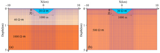
Figure 6.
Sketch map of different water body models. (a) In Model A, the water body is situated on sedimentary strata with a similar resistivity, and (b) in Model B, the water body is situated on bedrock with a significant resistivity difference. The light blue portion represents the water body, the orange portion represents strata with different resistivity, and the blue lines represent the forward mesh.
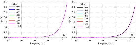
Figure 7.
Comparison of the magnetic field at different positions in (a) Model A and (b) Model B.
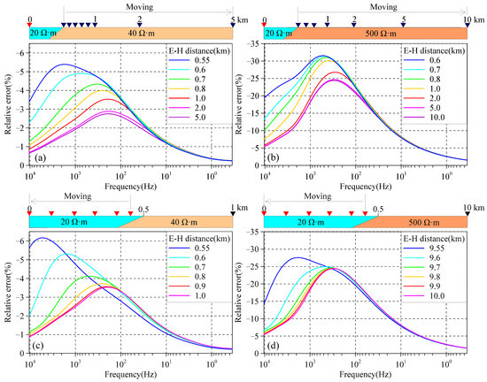
Figure 8.
Comparison of the relative error of the magnetic field with different distances between separated electric and magnetic channels. (a,b) The measuring point is located at the center of the water body while the magnetic channel moves along the shore in Model A (a) and Model B (b); (c,d) the measuring point moves over the water while the magnetic channel is located at 1.0 km in Model A (c) and 10.0 km in Model B (d). The red inverted triangle represents the measuring point over the water (colored in light blue), the black inverted triangle represents the magnetic channel on the shore (colored in orange), and the E-H distance in the legend denotes the distance between the separated electric and magnetic channels.
As observed in Figure 7, the magnetic field along the profile increases as the frequency decreases, and the magnetic field remains relatively consistent at different locations. This indicates that the electrical difference between the water and shore has minimal impact on the horizontal component of the total magnetic field in these two models. Figure 8 displays the relative error of the magnetic field of Models A and B. It can be observed that the magnetic field on the shore is lower than that at the measuring point over the water. As the separated electric and magnetic channels move further apart, the relative error of the magnetic field initially increases and then decreases with the decrease in the frequency, primarily concentrated in the middle-high frequency band. With an increase in the distance between the separated electric and magnetic channels, the peak value of the relative error of the magnetic field gradually decreases and shifts from the high-frequency band toward the middle-frequency band.
For Model A, in Figure 8a, the measuring point is located at the center of the water area, and the magnetic channel gradually moves from the shore, increasing the distance between the separated electric and magnetic channels. When the magnetic channel is 0.05 km away from the shore, the distance between the separated electric and magnetic channels is 0.55 km, and the relative error of the magnetic field slightly exceeds 5% in the frequency band around 1 k–4 k Hz. As the magnetic channel continues to move away from the shore, the distance between the separated electric and magnetic channels increases, leading to a decrease in the relative error, and the main part moves from the high-frequency band to the middle-frequency band. When the magnetic channel is 4.5 km away from the shore, the distance between the separated electric and magnetic channels is 5.0 km, and the relative error of the magnetic field tends to stabilize (<3%). In Figure 8c, with the magnetic channel fixed at 1.0 km, the measuring point over the water gradually approaches the water’s center from the shore, increasing the distance between the separated electric and magnetic channels. When the measuring point over the water is within 0.1 km from the shore, the distance between the separated electric and magnetic channels is less than 0.6 km, and the relative error of the local frequency band above 1 k Hz exceeds 5%. As the measuring point moves towards the water’s center, the distance between the separated electric and magnetic channels gradually increases, leading to a decrease in the relative error of the magnetic field, and the main part moves from the high-frequency band to the middle-frequency band. When the measuring point is 0.5 km away from the shore, the distance between the separated electric and magnetic channels is 1.0 km, and the relative error of the magnetic field tends to stabilize (<3%). From the above analysis, it is evident that whether the measuring point or the magnetic channel is close to the shore, the relative error of the magnetic field between the magnetic channel and the measuring point increases, indicating that the electrical difference between the media on both sides of the shore is the primary factor causing the magnetic field difference.
For Model B, as seen in Figure 8b,d, the relative error variation of the magnetic field with the distance between the separated electric and magnetic channels is similar to that in Model A. However, due to the significantly higher land resistivity compared to the water, the relative error of all frequencies above 3 Hz exceeds 5%. In Figure 8b, with the measuring point fixed at the center of the water area, the magnetic channel gradually moves away from the shore, increasing the distance between the separated electric and magnetic channels. When the magnetic channel is 0.1 km away from the shore, the distance between the separated electric and magnetic channels is 0.6 km, and the maximum relative error reaches 30%. As the magnetic channel moves away from the shore, when the distance between the separated electric and magnetic channels increases to 5.0 km, the relative error of the magnetic field tends to stabilize. However, the maximum relative error remains consistently close to 25%. In Figure 8d, the magnetic channel is fixed at 10.0 km, and the measuring point over the water gradually approaches the water center from the shore, resulting in a gradual increase in the distance between the separated electric and magnetic channels. When the distance between the electric and magnetic channels increases from 9.55 km to 10.0 km, the maximum relative error of the magnetic field decreases from 28% to 25%. Although the relative error of the magnetic field eventually stabilizes, it remains too high. Based on the above analysis, it can be seen that the significant electrical differences on two sides of the shore contribute to a high relative error of the magnetic field. Therefore, in this case, it is not suitable to replace the magnetic field of the measuring point over the water with the magnetic field on the shore.
4. AMT Observation Experiments Using Separated Electric and Magnetic Channels
We selected a river in Liaoning Province, China, for the AMT observation experiments using separated electric and magnetic channels. The river has a width of approximately 200–500 m and a depth of about 2–8 m, which satisfies the requirements for the observation experiments over the water. The Q sedimentary layers and sand–gravel mixed layers are mainly distributed on the surface. In the eastern part of the work area, there is a large area of granitic rocks, including Neoarchean and Late Triassic intrusive granitic gneiss and Late Jurassic biotite monzonitic granite [47]. Due to the significant transgression and seawater backflow, the river water is highly salinized. The resistivity of the Q sedimentary layer and the sand gravel layer ranges from several to over ten ohms, while the resistivity of the gneiss ranges from several hundred to thousands of ohms. The resistivity of the granitic bedrock is thousands of ohms, with obvious electrical differences. Since there is a similarity in the resistivity between the river water and the surface strata near the shore, the magnetic field in the river can be approximated by that on the Q sedimentary layer and the sand gravel layer near the shore.
4.1. Magnetic Channel Comparison Experiment
Figure 9 shows the work area of the AMT observation experiment and the arrangement of electric channels in the river. We set the measuring point at the center of the river for the electrical field and selected three magnetic channel sites (M1, M2, and M3) on the shore, which were located at distances of 0.1 km, 0.3 km, and 0.8 km from the shore, respectively. The corresponding distances between the separated electric and magnetic channels were 0.3 km, 0.5 km, and 1.0 km, respectively. In the experiment, the polar distances of 20 m and 60 m were selected, with an observation time of 45 min. The observation frequency range was 0.35–10,400 Hz. The apparent resistivity and impedance phase curves were obtained as presented in Figure 10.
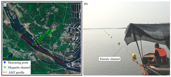
Figure 9.
AMT observation experiment using separated electric and magnetic channels in a river in Liaoning province, China: (a) the work area and (b) the electric channel arrangement in the river.
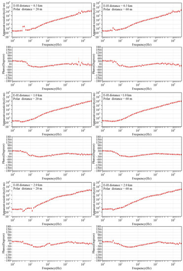
Figure 10.
Apparent resistivity and impedance phase curves of AMT at different magnetic channel sites on the shore. The E-H distance represents the distance between the separated electric and magnetic channels.
Figure 10 displays the apparent resistivity and impedance phase curves of AMT survey at different magnetic channel sites. The apparent resistivity curves exhibit a “low–middle–high” electrical pattern, which aligns with the underground geological and petrophysical variation in the work area, indicating the reliability of the obtained data. As we can see, the apparent resistivity and impedance phase curves obtained at three different magnetic channel sites exhibit good quality. However, the data’s robustness in the high-frequency band of 1 k–4 k Hz and the low-frequency band around 1.0 Hz is slightly poor. These two frequency bands are considered dead bands of the natural source, resulting in a low signal-to-noise ratio. Additionally, since the magnetic channel site M1 is close to the river, the water flow is considered to affect the data in the low-frequency band. Nevertheless, the data curves observed at the three magnetic channel sites demonstrate good agreement, indicating that the magnetic field at the measuring point in the river is almost identical to that at the magnetic channel site on the shore. Thus, the use of the separated electric and magnetic channels observation mode is feasible. In Figure 10, it can be observed that when the distance between the separated electric and magnetic channels is greater than 0.5 km and the magnetic channel is located more than 0.3 km from the shore, the influence of river water and water flow on the magnetic field is likely minimal, resulting in good data quality that aligns with the results of forward modeling. Furthermore, when comparing the observation data with different polar distances, it becomes apparent that a large polar distance improves the signal-to-noise ratio of the data and allows for the acquisition of high-quality data.
4.2. Profile Experiment
We also conducted an AMT profile experiment using separated electric and magnetic channels in the same river. As shown in Figure 10, AMT profile AA’ was arranged in the mid-river and spanned a length of 2820 m. The profile consisted of 48 measuring points spaced 60 m, and the magnetic channel was located at site M2 on the shore (Figure 9). The V5-2000 MT equipment (Canada Phoenix Geophysics, Ltd., Scarborough, ON, Canada) was used for the experiment, with the observation frequency range of 0.35–10,400 Hz and the observation time of 45 min. Figure 11 presents the apparent resistivity and impedance phase curves of the AMT test profile, which generally correspond to those in Figure 10.
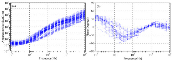
Figure 11.
(a) Apparent resistivity and (b) impedance phase curves of the AMT test profile in the river.
After editing the AMT data, we employed the 2D inversion software SCS2D (Zonge Engineering and Research Organization Inc., Tucson, AZ, USA) for profile inversion. The initial model used was a uniform half-space model with a resistivity of 100 Ω∙m. The top layer had a thickness of 5.0 m, and the row-to-row thickness multiplier was set to 1.25. A total of 20 layers were used, and the 2D moving-average filter parameter was set to 0.5. The maximum iteration was set to 20, and the error floor was 5% for the apparent resistivity and 50 milliradians for the impedance phase. The inversion frequency range was 1.0–10,400 Hz. Figure 12 displays the inversion results of the AMT test profile with transverse magnetic (TM) mode. The resistivity pseudo-section exhibits a “low–middle–high” characteristic from the surface. Based on the geological and petrophysical analysis of the study area, we conducted a preliminary interpretation of the inversion results. We identified three layers: the surface layer, which consists of salinized water, water-bearing silt, and sand gravel with a thickness of approximately 15–40 m; the middle layer, which is composed of gneiss with a thickness of approximately 25–120 m; and the deep layer, which is the granitic bedrock, being deeper in the east and shallower in the west, with the top depth of approximately 30–150 m.
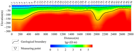
Figure 12.
Inversion results of the AMT test profile with TM mode in the river. The root-mean-square misfit is 1.34 after 12 iterations.
5. Discussion
Based on the forward simulation of two typical models and field experiments, it has been determined that the AMT observation technology using separated electric and magnetic channels over water-covered areas is feasible. However, the main factor contributing to data error is the electrical difference between the water and the shore. In cases where the resistivity of the water body is similar to that of the surrounding media, such as large rivers and lakes on sedimentary strata, the observation technology using separated electric and magnetic channels can be employed. However, when there is a significant resistivity difference between the water body and the surrounding media, such as large lakes and reservoirs on bedrock, this observation technology may yield lower exploration accuracy.
To mitigate the influence of the electrical difference between the water and the shore under the separated electric and magnetic channels mode, both the electric and magnetic channels should be positioned at a certain distance from the shore. This distance should increase with the increase in the electrical difference between the water and the shore. Before AMT detection, the magnetic channel site can be selected through numerical simulation and field observation experiments. For rivers and lakes that are not suitable for the observation technology using separated electric and magnetic channels, exploration accuracy may be reduced, or the electric and magnetic fields should be observed synchronously at the same site. However, this approach requires advanced geophysical equipment.
The field experiments conducted in the river further confirmed the feasibility of the observation technology using separated electric and magnetic channels. Since the resistivities of the river and the shore were similar, and the river was shallow, the magnetic field in this study area was relatively uniform. The magnetic field on the shore could effectively replace the magnetic field in the river, as demonstrated by the observation experiments. However, the low-frequency vibration caused by the river flow might affect the data quality. Unfortunately, due to equipment limitations, we could not directly observe the magnetic field in the river, making it difficult to accurately evaluate the accuracy of the measured data.
6. Conclusions
This paper introduced an AMT observation technology using separated electric and magnetic channels over water-covered areas. The distribution characteristics of the magnetic field error caused by this observation technology were discussed through forward simulation. Field experiments were conducted at the estuary of a river in Liaoning Province, China, to validate the feasibility of the AMT observation technology. The results demonstrate that the proposed AMT observation technology is practical and provides an effective method for surveying mineral resources and engineering exploration in aquatic environments.
When conducting AMT exploration in aquatic environments, the observation technology of separated water–electric and land–magnetic channels proves to be useful and feasible. The magnetic channel should be positioned in a quiet area on the shore, at a certain distance from the shore, to minimize the influence of electrical differences between the water and the shore. The selection of a suitable area for the magnetic channel can be determined through numerical simulation and field experiments. However, there are still some limitations to the AMT observation technology presented in this paper. Ongoing efforts are being made to develop AMT observation technologies and equipment for aquatic environments [48], which are expected to enhance the performance of mineral exploration and engineering exploration over water-covered areas.
Author Contributions
Conceptualization, Q.W. and H.-Z.M.; Methodology, Q.W. and Y.-B.L.; Software, Y.-B.L. and G.W.; Supervision, Y.-B.L. and H.-Z.M.; Validation, Y.-B.L., H.-Z.M., G.W. and Z.-Y.Z.; Writing—original draft, Q.W. and Z.-Y.Z.; Writing—review and editing, Q.W., Y.-B.L., H.-Z.M., G.W. and Z.-Y.Z. All authors have read and agreed to the published version of the manuscript.
Funding
This research was funded by the Basic Scientific Research Project of the Chinese National Non-profit Institute (AS2022P02, AS2019P01, YYWF201732).
Data Availability Statement
Data associated with this research are available and can be obtained by contacting the corresponding author.
Acknowledgments
We are thankful for the constructive comments of the editors and anonymous reviewers that improved this paper. We are also grateful for the useful advice for field experiments provided by Shumin Wang.
Conflicts of Interest
The authors declare no conflict of interest.
References
- Teng, J.W. Strengthening exploration of metallic minerals in the second depth space of the crust, accelerating development and industrialization of new geophysical technology and instrumental equipment. Prog. Geophys. 2010, 25, 729–748. [Google Scholar]
- Xue, G.; Chen, W.; Wu, X.; Yan, S.; Guo, W. A Near-Source Electromagnetic Method for Deep Ore Explorations. Minerals 2022, 12, 1208. [Google Scholar] [CrossRef]
- Zhang, P.X. Salt Lakes in Qaidam Basin, 1st ed.; Science Publishing House: Beijing, China, 1987; pp. 143–148. [Google Scholar]
- Liu, C.L.; Jiao, P.C.; Wang, M.L. A tentative discussion on exploration model for potash deposits in basins of China. Miner. Depos. 2010, 29, 581–592. [Google Scholar]
- Wang, K.; Zhang, Y.; Han, J.H.; Ma, L.C.; Zheng, M.P.; Wu, Y.; Yang, B.W. Distribution and Genesis of Potassium-Bearing Minerals in Lop Nor Playa, Xinjiang, China. Minerals 2023, 13, 560. [Google Scholar] [CrossRef]
- Cagniard, L. Basic theory of the magnetotelluric method of geophysical prospecting. Geophysics 1953, 63, 605–636. [Google Scholar] [CrossRef]
- Filloux, J.H. Techniques and instrumentation for the study of natural electromagnetic induction at sea. Phys. Earth Planet. Inter. 1973, 7, 323–338. [Google Scholar] [CrossRef]
- Bnnett, D.J.; Filloux, J.H. Magnetotelluric deep electrical sounding and resistivity. Rev. Geophys. Space Phys. 1975, 13, 197–203. [Google Scholar] [CrossRef]
- Filloux, J.H. North pacific magnetotelluric experiments. J. Geomagn. Geoelectr. 1980, 32, SI33–SI43. [Google Scholar] [CrossRef]
- Chave, A.D.; Filloux, J.H. Electromagnetic induction field in the deep ocean off California: Oceanic and ionospheric sources. Geophys. J. Int. 1984, 77, 143–171. [Google Scholar] [CrossRef]
- Eidesmo, T.; Ellingsrud, S.; MacGregor, L.M.; Constable, S.; Sinha, M.C.; Johansen, S.; Kong, F.N.; Westerdahl, H. Sea bed logging (SBL), a new method for remote and direct identification of hydrocarbon filled layers in deepwater areas. First Break 2002, 20, 144–152. [Google Scholar]
- Constable, S. Ten years of marine CSEM for hydrocarbon exploration. Geophysics 2010, 75, 75A67–75A81. [Google Scholar] [CrossRef]
- Key, K. Marine electromagnetic studies of seafloor resources and tectonics. Surv. Geophys. 2012, 33, 135–167. [Google Scholar] [CrossRef]
- Constable, S. Review paper: Instrumentation for marine magnetotelluric and controlled source electromagnetic sounding. Geophys. Prospect. 2013, 61, 505–532. [Google Scholar] [CrossRef]
- Li, T.L.; Lin, J.; Wang, D.P.; Liu, C.F.; Zeng, X.Z. Study on Sea-Land Electromagnetic Noise and Beach Magnetotelluric Sounding, 1st ed.; Geophysics Publishing House: Beijing, China, 2001; pp. 79–92. [Google Scholar]
- Deng, M.; Liu, F.L.; Zhang, Q.S.; Chen, K. Long-span and Multi-point Synchronizing Data Acquisition for Seafloor Magnetotelluric Based on Union of Marine and Land. Sci. Technol. Rev. 2006, 24, 28–32. [Google Scholar]
- He, Z.X.; Sun, W.B.; Kong, F.S.; Wang, X.F. Marine electromagnetic approach. Oil Geophys. Prospect. 2006, 41, 45l–457. [Google Scholar]
- Li, Y.G.; Constable, S. Transient electromagnetic in shallow water: Insights from 1D modeling. Chin. J. Geophys. 2010, 53, 737–742. [Google Scholar]
- Shen, J.S.; Zhan, L.S.; Wang, P.F.; Ma, C.; Lian, F.M. Theoretic analysis and numerical simulation of effects of airwave interaction on the marine controlled source electromagnetic exploration. Chin. J. Geophys. 2012, 55, 2473–2488. [Google Scholar]
- Yin, C.C.; Ben, F.; Liu, Y.H.; Huang, W.; Cai, J. MCSEM 3D modeling for arbitrarily anisotropic media. Chin. J. Geophys. 2014, 57, 4110–4122. [Google Scholar]
- Yang, J.; Liu, Y.; Wu, X.P. 3D simulation of marine CSEM using vector finite element method on unstructured grids. Chin. J. Geophys. 2015, 58, 2827–2838. [Google Scholar]
- Nyquist, J.E.; Freyer, P.A.; Toran, L. Stream bottom resistivity tomography to map ground-water discharge. GroundWater 2008, 46, 561–569. [Google Scholar] [CrossRef]
- Tsourlos, P.; Tsokas, G.N. Underwater resistivity surveying for sludge layer parametrization. In Proceedings of the 1st International Conference on Advances in Mineral Resources Management and Environmental Geotechnology, Crete, Greece, 7–9 June 2004. [Google Scholar]
- Dahlin, T.; Loke, M.H. Underwater ERT surveying in water with resistivity layering with example of application to site investigation for a rock tunnel in central Stockholm. Near Surf. Geophys. 2018, 16, 230–237. [Google Scholar] [CrossRef]
- Mollidor, L.; Tezkan, B.; Bergers, R.; Löhken, J. Float-transient electromagnetic method: In-loop transient electromagnetic measurements on Lake Holzmaar, Germany. Geophys. Prospect. 2013, 61, 1056–1064. [Google Scholar] [CrossRef]
- Byrdina, S.; Vandemeulebrouck, J.; Rath, V.; Silva, C.; Hogg, C.; Kiyan, D.; Viveiros, F.; Eleuterio, J.; Gresse, M. Resistivity structure of the Furnas hydrothermal system (Azores archipelago, Portugal) from AMT and ERT imaging. In Proceedings of the EGU General Assembly Conference, Vienna, Austria, 17–22 April 2016. [Google Scholar]
- Yogeshwar, P.; Küpper, M.; Tezkan, B.; Rath, V.; Kiyan, D.; Byrdina, S.; Cruz, J.V.; Andrade, C.; Viveiros, F. Innovative Boat-Towed Transient Electromagnetics-Investigation of the Furnas Volcanic Lake Hydrothermal System, Azores. Geophysics 2019, 85, 41–56. [Google Scholar] [CrossRef]
- Liu, J.X.; Mao, X.C.; Zhang, Y.S. Underwater magnetotelluric sounding method. Geophys. Geochem. Explor. 1997, 21, 74–76. [Google Scholar]
- Ding, J.R.; Wang, Y.; Yu, P.; Wang, J.L.; Hao, T.Y. MT Surveying Test of Synchronous Acquisition by Separated Electric and Magnetic Channels on Shallow Sea. Oil Geophys. Prospect. 2006, 41, 107–110. [Google Scholar]
- Yang, S. Computation of Apparent Resistivity for Separately Acquired Electromagnetic Signals in MT Exploration of Water Domain. Oil Geophys. Prospect. 2006, 41, 592–595. [Google Scholar]
- Xu, J.R.; Liu, J.X.; Li, A.Y.; Yang, S.; Liu, H.F.; Weng, J.B. Liquid effect upon electromagnetic fields in water area MT exploration. J. Cent. South Univ. Sci. Technol. 2007, 38, 567–573. [Google Scholar]
- Feng, N.; Tong, T.G.; Zuo, G.Q. The Application of dual-frequency IP in engineering geological survey on water area. West-China Explor. Eng. 2006, 18, 187–188. [Google Scholar]
- Ni, L.; Chen, D.H.; Xu, H.W.; Zhang, H.; Jin, W.J.; Zhang, W.H.; Lin, D.M. Electrical exploration on water region used in the geophysical prospecting cross the river and lake. Prog. Geophys. 2012, 27, 2710–2715. [Google Scholar]
- Liu, H.Y. The application of DC resistivity to shallow marine engineering exploration. Geophys. Geochem. Explor. 2013, 37, 756–760. [Google Scholar]
- Fu, X.M.; Tan, X.J.; Lei, Y.C. The Application of Integrated Geophysical Methods to Water Crossing Project. Chin. J. Eng. Geophys. 2013, 10, 175–179. [Google Scholar]
- Zhang, Y.S.; Li, B.; Zhang, J.L. The application of the transient electromagnetic method to the waters geological investigation. Geophys. Geochem. Explor. 2016, 40, 160–162. [Google Scholar]
- Meng, Q.L. Application of towing transient electromagnetic method of waters in the geological investigation of the Muping Xiangjiang Bridge. In Proceedings of the 2018 National Engineering Survey Conference, Xi’an, China, 21–24 June 2018. [Google Scholar]
- Jiang, J. Application of towed TEM method in shallow waters geotechnical investigation. Coal Geol. China 2019, 31, 103–107. [Google Scholar]
- Qi, P.; Yin, Y.; Jin, S.; Wei, W.; Xu, L.; Dong, H.; Huang, J. Three-Dimensional Audio-Magnetotelluric Imaging including Surface Topography of the Cimabanshuo Porphyry Copper Deposit, Tibet. Minerals 2021, 11, 1424. [Google Scholar] [CrossRef]
- Pitiya, R.; Lu, M.; Chen, R.; Nong, G.; Chen, S.; Yao, H.; Shen, R.; Jiang, E. Audio Magnetotellurics Study of the Geoelectric Structure across the Zhugongtang Giant Lead–Zinc Deposit, NW Guizhou Province, China. Minerals 2022, 12, 1552. [Google Scholar] [CrossRef]
- Wang, N.; Wang, Z.; Sun, Q.; Hui, J. Coal Mine Goaf Interpretation: Survey, Passive Electromagnetic Methods and Case Study. Minerals 2023, 13, 422. [Google Scholar] [CrossRef]
- Zhang, Q.S.; Wang, J.Y.; Ye, J.Y.; Wang, L. A feasibility test of offshore magnetotelluric prospecting in the Leiqiong area. Geol. Prospect. 2006, 42, 64–67. [Google Scholar]
- Chen, L.S.; Wang, G.E. Magnetotelluric Sounding Method, 1st ed.; Geophysics Publishing House: Beijing, China, 1990; pp. 10–22. [Google Scholar]
- Hermance, J.F.; Thayer, R.E. The telluric-magnetotelluric method. Geophysics 1975, 40, 664–668. [Google Scholar] [CrossRef]
- Stodt, J.A.; Hohmann, G.W.; Ting, S.C. The telluric-magnetotelluric method in two- and three-dimensional environments. Geophysics 1981, 46, 1137–1147. [Google Scholar] [CrossRef][Green Version]
- Coggon, J.H. Electromagnetic and electrical modeling by the finite element method. Geophysics 1971, 36, 132–151. [Google Scholar] [CrossRef]
- Bureau of Geology and Mineral Resources of Liaoning Province. Regional Geology of Liaoning Province, 1st ed.; Geophysics Publishing House: Beijing, China, 1989; pp. 252–257. [Google Scholar]
- Zhao, Y.; Chen, X.D.; Huang, Y.; Wang, G.; Li, Y.B.; Zhao, F.G.; Wang, S.M. The development of three-component inductive magnetic field sensor suitable for shallow water work. Geophys. Geochem. Explor. 2019, 43, 1326–1332. [Google Scholar]
Disclaimer/Publisher’s Note: The statements, opinions and data contained in all publications are solely those of the individual author(s) and contributor(s) and not of MDPI and/or the editor(s). MDPI and/or the editor(s) disclaim responsibility for any injury to people or property resulting from any ideas, methods, instructions or products referred to in the content. |
© 2023 by the authors. Licensee MDPI, Basel, Switzerland. This article is an open access article distributed under the terms and conditions of the Creative Commons Attribution (CC BY) license (https://creativecommons.org/licenses/by/4.0/).