Abstract
This paper introduces an original approach to the joint inversion of airborne electromagnetic (EM) data for three-dimensional (3D) conductivity and chargeability models using hybrid finite difference (FD) and integral equation (IE) methods. The inversion produces a 3D model of physical parameters, which includes conductivity, chargeability, time constant, and relaxation coefficients. We present the underlying principles of this approach and an example of a high-resolution inversion of the data acquired by a new active time domain airborne EM system, TargetEM, in Ontario, Canada. The new TargetEM system collects high-quality multicomponent data with low noise, high power, and a small transmitter–receiver offset. This airborne system and the developed advanced inversion methodology represent a new effective method for mineral resource exploration.
1. Introduction
Induced polarization effects have been documented in induced sources since the late 1980s [1,2]. In 1996, Smith and Klein [3] first identified these effects in airborne data. At that time, they were regarded as a special case and not to be generally considered when interpreting airborne EM data. Since that time, airborne systems have evolved, and system signal-to-noise ratios have dramatically increased so that induced polarization effects are routinely observed in the raw data ([4,5,6,7,8], etc.). Indeed, we are now to the point where it has been shown that quantitative interpretation or inversion cannot be conducted accurately without including these effects [9,10].
The current topic of research is not whether there are IP effects in AEM data but how best to incorporate them into the interpretation schemes. For a zero offset time domain system, induced polarization is the only mechanism that can cause the vertical component of the response to become negative. Because of this, various metrics, such as the first channel to become negative or the integral of the negative part of the transients, have been used to estimate the magnitude of the induced polarization. These types of data space metrics can be used as a quick and dirty first look at the data to determine if induced polarization effects are present. Still, the lack of negative transients does not preclude polarizable media. Several methods that extend the interpretations to the model space include Kwan [11], who presents a method where a global search is conducted for a best fit resistive and chargeable half-space, essentially developing maps of apparent resistivity and chargeability. Chen [12] decomposes the observed decay curves into a resistive and a chargeable part to identify locations where IP is likely contained in the data. Macnae [13] uses a set of thin sheets as basis functions to recover all Cole-Cole parameters and includes superparamagnetism as a bonus.
As with conductivity-only interpretation, much of the thrust has been moving towards the one-dimensional (1D) approximation, where for each transmitter–receiver location, the approximation is made that the Earth is laterally invariant for forward modeling and sensitivity calculations. This speeds up and simplifies the computations and is a form of regularization (stabilization) since the class of models recovered by the inversion is greatly simplified. Works conducted by [7,14,15,16] have all demonstrated the effectiveness of these inversion methods with good case histories. However, it is known that conductivity-only 1D inversions can create spurious results [17], and including induced polarization will not change this. Additionally, the inline component of the dB/dt field, which has been shown to greatly reduce non-uniqueness and improve resolution in inversion results, cannot be used with the 1D approximation.
The first demonstration of using a full, rigorous 3D inversion of airborne data for IP parameters was given by Goold et al. [18]. Using a numerical modeling study and field data inversion, the authors of this paper demonstrated the possibility of developing an airborne version of the spectral IP method. Kang and Oldenburg [19] also used full three-dimensional models of the electric fields for recovering distributed IP information from an inductive source. This method produced excellent results over a known kimberlite [8]. However, it is a multi-step process that uses early time data to build a conductivity model, which is forward modeled to synthesize the full decay, removes this decay from the observed data, and then inverts the residual for pseudo-changeability. This approach is robust, but the resistivity and chargeability are not truly separable, and early times are often influenced by polarizable media.
The paper by [9] is an excellent overview of the effects of varying Cole-Cole parameters on the measured airborne response from a 1D perspective. For inversion purposes, the takeaway from this paper is that the inversion problem is highly non-linear and non-unique, more so than conductivity-only airborne inversion problems. Therefore, a knowledgeable processor, robust workflow, and reconciling the results with geology are of the utmost importance [20]. This study of 1D modeling and inversion also shows that because of the limited bandwidth of airborne EM systems, the recovered time constant of chargeability is between 1 × 10⁻² and 1 × 10⁻⁴ s. This result is in general agreement with [13] and our personal experience.
The aforementioned papers make approximations with the modeling physics, dimensionality, or both to recover a subsurface physical parameter model. Cox et al. [10] developed a method of full 3D simultaneous inversion for conductivity and other IP parameters based on the generalized effective medium theory of the IP effect GEMTIP [21]. In that paper, the integral equation (IE) method was used for 3D modeling. Here, we extend the modeling and inversion code to use a hybrid finite difference (FD) and IE modeling scheme and develop a new methodology to reduce the chance of being trapped in a local minimum in the parametric functional. We create a more robust result by building up the model dimensionality step-by-step. Our workflow progresses from apparent resistivities and polarization parameters to 1D inversion and to full 3D inversion. If the 1D results are sufficient to fit all components of the data, the 3D modeling will reveal this. If the model does not fit the data, as is nearly always the case, the 3D inversion will adjust the model to fit the data, but with a minimum departure from the 1D inversion results to accomplish this, as dictated by the stabilizer. All data from the AEM system, including all time channels and components (inline and vertical), contribute to this 3D modeling and inversion process and are fitted in this methodology.
The recently developed TargetEM active airborne EM system data are used for the case history. This system was developed to image discrete conductors and layering. The system prioritizes precise, detailed analysis through a combination of low noise, robust power, and a zero-offset transmitter–receiver setup. By using cutting-edge electronic components and incorporating a sophisticated suspension system within the receiver complemented by a bucking coil designed to compensate for the direct impact of the primary field, the system achieves a higher than ordinary signal-to-noise ratio. The transmitting pulse features a rectangular waveform with a short turn-off time providing a clean secondary field response.
2. Methods
2.1. TargetEM System Description
TargetEM represents an innovative airborne electromagnetics system currently under patent review. It employs full waveform recording at a rate of 73,728 Hz. The system achieves a maximum dipole moment of 700,000 NIA (number of turns multiplied by the peak current and multiplied by the transmitter area), depending on the transmitter loop’s diameter and the number of turns. Typically, the loop diameter ranges from 21 m to 31 m, with a base frequency of either 25 or 30 Hz, depending on the local powerline frequency. The system measures inline, crossline, and vertical dB/dt data (with processed B-field data also provided), within a time range spanning from 40 µs to 14 ms post-turn-off, varying with the base frequency and transmitter pulse width. It operates with a triaxial dB/dt receiver located in the center of the horizontal transmitter loop, with a bucking coil collecting both VLF and AFMAG data alongside the time-domain EM data [22].For this survey, a loop of 21 m was used. The data were processed to 37 Z component channels from 41 μs to 8.2 ms and 21 X component channels from 514 μs to 8.2 ms (centers after waveform turn off). The waveform is a trapezoid with a peak current of 240 A. The turn-off time is 1.0 ms. All time channels and components were used in the inversion. The units of the system are pV/Am4. This is the same as pT/sAm2, or equivalently, the time derivative of the magnetic field normalized by the transmitter dipole moment.
2.2. Induced Polarization Parameterization
For apparent model parameters, 1D inversion and 3D inversion, modeling occurs in the frequency domain. The fields are transformed to the time domain with a cosine transform and then convolved with the time derivative of the instrument’s current waveform to arrive at the time domain response [23]. This approach facilitates the inclusion of flexible induced polarization (IP) parameterization within the modeling and inversion processes. The simplified GEMTIP model [21] is used, which is similar to the Cole-Cole model [24] and is utilized to parameterize induced polarization effects:
where is the DC conductivity (S/m), ω is the angular frequency (rad/s), τ is the time constant; is the intrinsic chargeability, and C is the dimensionless relaxation parameter. The dimensionless intrinsic chargeability, η, characterizes the intensity of the IP effect.
2.3. Model Discretization
For both 1D and 3D methods, a 3D model is discretized into voxels horizontally and vertically. Typically, 25 m cells are used in the inline direction, and 25–50 m cells are used in the crossline direction. Vertically, around 20 cells are logarithmically spaced from 3 m to 70 m. The discretization of the model can, of course, be adjusted with varying systems, geology, time gates, line spacings, etc., to capture the full resolution of the system. It can also be changed on each increase in modeling dimensionality with interpolation, but the important fact is that a 3D volume of stabilized model parameters is used during each step, ensuring a coherent model.
2.4. Global Search for Apparent Parameters
A global search is first performed on the vertical component decay of each sounding location to find the best fitting GEMTIP parameters (conductivity, chargeability, time constant, relaxation coefficient) for each location. These are equivalent to “apparent” parameters. The best-fit determination uses weighted data, where each datum is weighted by the inverse of the estimated error:
where is the total error, is the estimated percent error, and is the estimated absolute error. Data with a magnitude less than 1/3rd of the error floor are rejected completely. For this survey, the data errors were estimated to be 10% of the observed value plus 0.003 pV/Am4 for the Z channel and 0.01 pV/Am4 for the X channel. These should not necessarily be taken as actual data error but estimates that produce the best inverse images and visual data fit at an RMS = 1. These errors include system noise and errors from sources such as incorrect altitude and instrument tilt. The best-fit parameters are interpolated onto the discretized 3D grid. This forms the starting and reference model for the 1D inversion.
2.5. Inversion Method
Both the 1D and 3D inversions attempt to minimize the parametric functional [25]:
where is the data weighting matrix, is the forward modeling operator, is a stabilizing functional, and is the regularization parameter. Equation (3) is minimized with the reweighted regularized conjugate gradient (RRCG) method, as described in [26]. The practical implementation of the RRCG method requires effective algorithms for forward modeling and sensitivity (Fréchet derivative) calculations. Below, we discuss the corresponding techniques used for 1D and 3D inversions.
2.6. One-Dimensional Modeling and Inversion
The 1D modeling uses the layered Earth expressions from [27] to find the vertical component of the frequency domain field (the inline and crossline components are null and cannot be used in 1D inversion). The 1D sensitivities for inversion are found via perturbation of the DC conductivity, and then the sensitivities for the GEMTIP parameters are found via the chain rule from the analytical derivatives of Equation (1), so almost no additional computation time is required to fully include induced polarization in the modeling and sensitivity calculation [10]. While the sensitivities are 1D, the mesh on which the inversion operates is 3D. Hence, the stabilizers are 3D, which is similar to the laterally or spatially constrained inversion of [28]. A variety of stabilizers could be used in any combination, including minimum norm, first or second derivatives, and focusing [25]. Here, we are using a second derivative stabilizer for all inversions.
The 1D inversion is run to the approximate error level in the data (normalized RMS = 1). As with all inverse problem solutions, many inversions are run with different parameters to determine the robustness of the model and to select the parameters that best allow data fit, convergence, and a geologically reasonable model. For example, between 16 and 30 layers are used in the 1D inversion. The exact number depends on the target (e.g., is resolving variable overburden thickness important?), the system resolution (how early are instrument time samples valid?), and what is required to fit the data properly.
2.7. Three-Dimensional Modeling and Inversion Using Hybrid Finite Difference and Integral Equation Method
We use the 1D inversion results to create a starting and reference model for the 3D inversion. The model from the 1D inversion undergoes a smoothing process through convolution using a boxcar function, which matches the lateral extent of the instrument’s sensitivity domain (footprint). This approach is rooted in the idea that within the instrument’s footprint, where the Earth displays lateral uniformity, the 1D approximation generates reasonable models. Consequently, smoothing in these regions does not significantly alter the model. However, when the lateral variations are pronounced, the 1D inversion tends to present artifacts and inaccurate geometry and conductivity differences that are too weak. In such instances, smoothing the 1D model establishes general regional conductivity, serving as a background and starting model for the subsequent 3D inversion.
The 3D modeling and sensitivity calculations are based on the hybrid finite difference (FD) and integral equation (IE) method [29,30]. This technique employs an anomalous field formulation where the total field is split into background and anomalous fields,
The anomalous electric field, in the frequency domain is related to the background electric field, according to the following second-order differential equation:
where and represent the total and anomalous electric conductivities of the medium, respectively.
Equation (5) is discretized on the staggered grid and is solved using the conventional finite difference technique [30,31]. Calculating the anomalous field with an equivalent source, represented by the right side of Equation (5), sidesteps issues linked to discretization problems from discrete sources. This method also streamlines the process of using complex sources, such as a loop versus a vertical dipole or an arbitrarily oriented dipole. Widely referenced in EM modeling literature, this approach is adaptable across various methods like FD, finite volume, finite element, or IE methods [32].
We employ the Paradiso direct solver [33] to solve for multiple sources and their adjoint counterparts efficiently. The advantage of a direct solver is that the left-hand side of Equation (5), which is independent of the source, can be decomposed once, and then solutions for multiple right-hand sides can be solved with little additional effort. This is especially advantageous for airborne EM modeling and inversion because there are a very large number of sources (transmitter positions) and adjoint sources (receiver positions and components), each with a unique right-hand side. Solving these iteratively has proved challenging from a computation time perspective because each source requires a completely independent solving run.
Once the anomalous field is calculated, the fields at the receivers must be found. To speed up and stabilize the computations, we use the approach generally reserved for the IE method to calculate the magnetic fields at the receivers. The anomalous magnetic fields at the receiver position, , can be expressed as an integral over the excess currents in the inhomogeneous domain D:
where is the magnetic Green’s tensor defined for an unbounded conductive medium with the background (horizontally layered) anisotropic conductivity; is the total electric field at the point inside the domain, and is the anomalous (scattered) magnetic field at receiver .
The inversion is run using the RRCG method for conductivity, chargeability, time constant, and relaxation parameter, as outlined by [10]. The sensitivities are found using reciprocity for the DC conductivity, and then the sensitivities for the GEMTIP parameters are found using the chain rule (analytic derivatives of Equation (1)).
In summary, the methodology for the 3D inversion of airborne data consists of the following steps:
- 1.
- Determine the best-fit polarizable half-space for each transmitter–receiver pair, including conductivity, chargeability, time constant, and relaxation coefficient;
- 2.
- Grid the best-fit half-spaces into a 3D voxel model;
- 3.
- Use this as a starting point for inversion based on a one-dimensional (1D) approximation;
- 4.
- Smooth the 1D inversion results;
- 5.
- Run the 3D inversion using the smoothed 1D inversion results as a starting and reference model.
All inversions in this example were run on a standard desktop with 64 GB of RAM and an Intel 3.7 GHz Quad Core I7. The main language is MATLAB R2023b, utilizing the parallel computing toolbox to speed up certain blocks. Generally, using a relatively polished workflow, the full inversion process takes a few hours from start to finish.
3. Results
3.1. Geologic Background
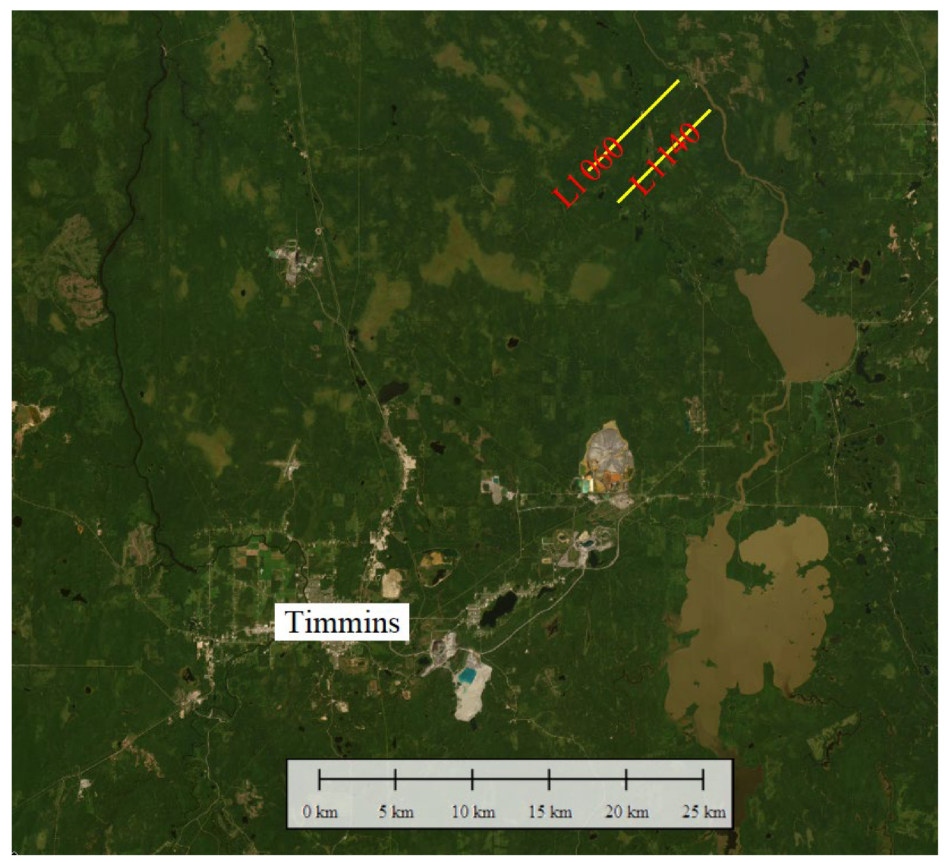
The study area is in the Porcupine Mining District, around 40 km north of Timmins, Northern Ontario. The district is undergoing gold and nickel prospecting with historic geophysical ground and airborne surveys [34]. The property lies in the Abitibi Terrain, eastern part of Superior Province, and is underlain by mafic and ultramafic rocks, as well as intermediate metavolcanics with iron formations. These early Precambrian units have been intruded by several metamorphosed mafic and ultramafic bodies. Thin inter-formational units of iron formations occur as sulfide and carbonate facies. Mafic to ultramafic intrusions range from gabbro to pyroxenite, peridotite, and dunite in composition. By the drill core observation, metavolcanic rocks are often hydrothermally brecciated in variable intensity. The area is extensively covered by quaternary glacial sediments. The overburden thickness may reach 30–50 m. Nearby drillholes conform the thickness of the overburden at 30 m with an intersection of sulfide mineralization at the depth between 80 and 103 m [34]. The geological terrain hosts some of the richest mineral deposits of the Superior Province, including the giant Kidd Creek massive sulfide deposit and the large gold camps of Ontario and Quebec [35]. The area is actively explored for sulfide nickel–copper–cobalt–PGE mineralization targets, VMS-Au, and potentially orogenic gold.
3.2. Survey
The TargetEM survey was flown along test lines of 1060 and 1140 in this area (Figure 1). The mean flight height was 53 m. Vertical (Z) component dB/dt data were processed to time channels from 41 μs to 8.24 ms, and the inline (X) component data from 514 μs to 8.24 ms. All time channels and components were used in the 3D inversion, and all-time channels from the vertical component were used in the 1D inversion. The two widely separated lines mean that the model was constrained in the crossline direction via heavy stabilization.
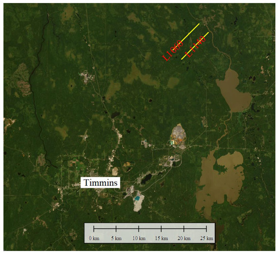
Figure 1.
Location map of the test TargetEM survey. The location of the two test lines L1060 and L1140 are shown.
3.3. Inversion Results
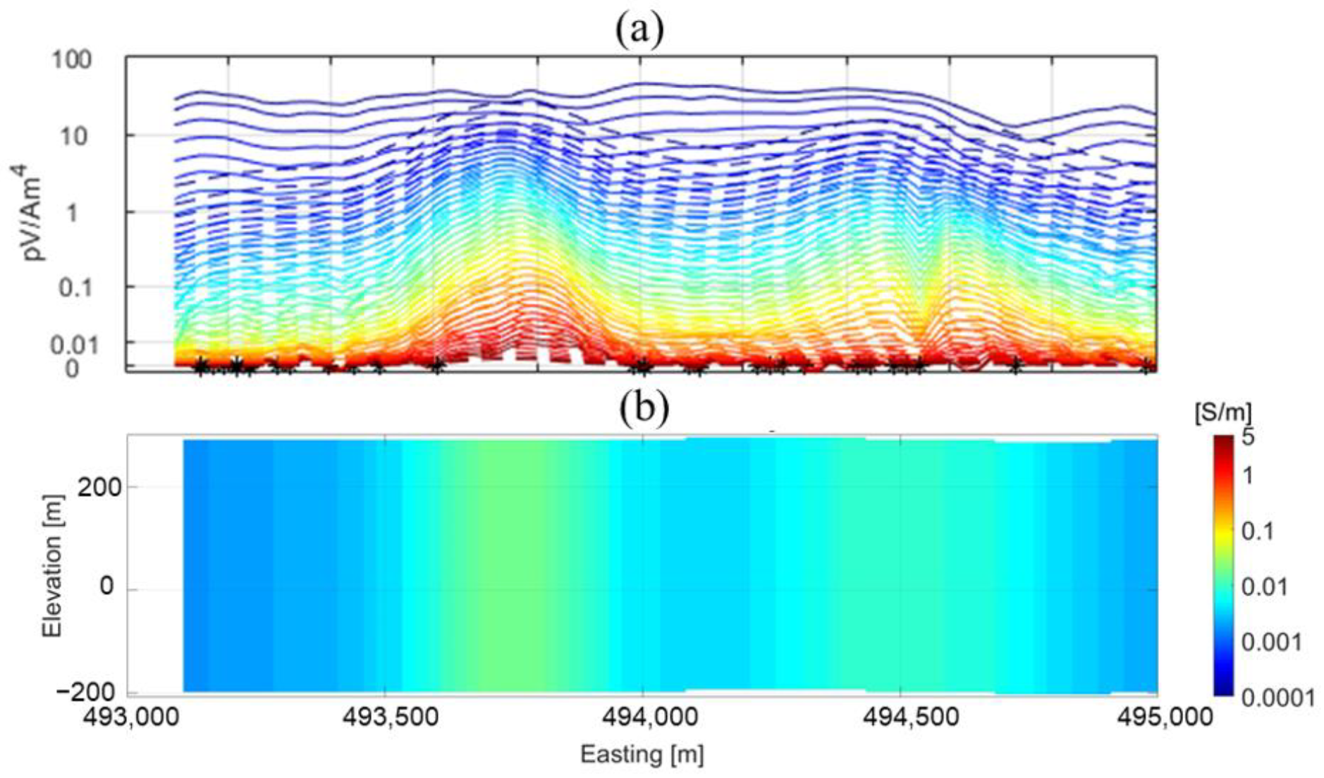
The results presented in the following figures are from each step in the methodology detailed above. For clarity, each parameter remains on the same color scale in each image despite the weaker contrast in the preliminary stages. Figure 2 shows the starting model produced by gridding the apparent model parameters from each station into a 3D model. In this case, we found a 20 mV/V half-space to be optimal as a starting model for the 1D inversion through testing and experience. This value is small enough to not create a large response, but large enough to generate some initial sensitivity to chargeability, relaxation coefficient, and time constant. The relaxation parameter C was set to 1 [unitless], and the time constant to 0.1 ms, which is near the center of the bandwidth of the system. The starting model is very smooth and is a rough approximation of the regional conductivity structure. It is close enough to provide the 1D inversion a starting and reference model. Note the data fit is reasonable for a starting model, but in no way close to the error level in the observed data.
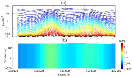
Figure 2.
Starting model and data fit. The top panel (a) shows the observed data (solid lines) and predicted data (dotted lines) of the vertical component as modeled using the 1D approximation. The time channels extend from 41 μs (blue) to 8247 µs (red). Black asterisks show rejected data points. The bottom panel (b) shows the apparent conductivity gridded into a 3D model and extracted along the line 1060. The data fit for the model shown is quite poor, as should be expected. The conductivity contrast in this model is weak, and the model is very approximate. This is the starting and reference model for the 1D inversion.
The predicted data shown in Figure 2 are from the 1D forward modeling approximation, as this is the starting point for the 1D inversion. It is important to remember that the data are not synthesized on the model as shown in the profile, but only on the column of cells directly under the modeled transmitter–receiver as if that conductivity structure extends laterally to infinity as a layered Earth. These 1D models are all merged or stitched into a single model parameter profile for display purposes. Conversely, 3D-modeled data are based on the conductivity structure shown in the Figures.
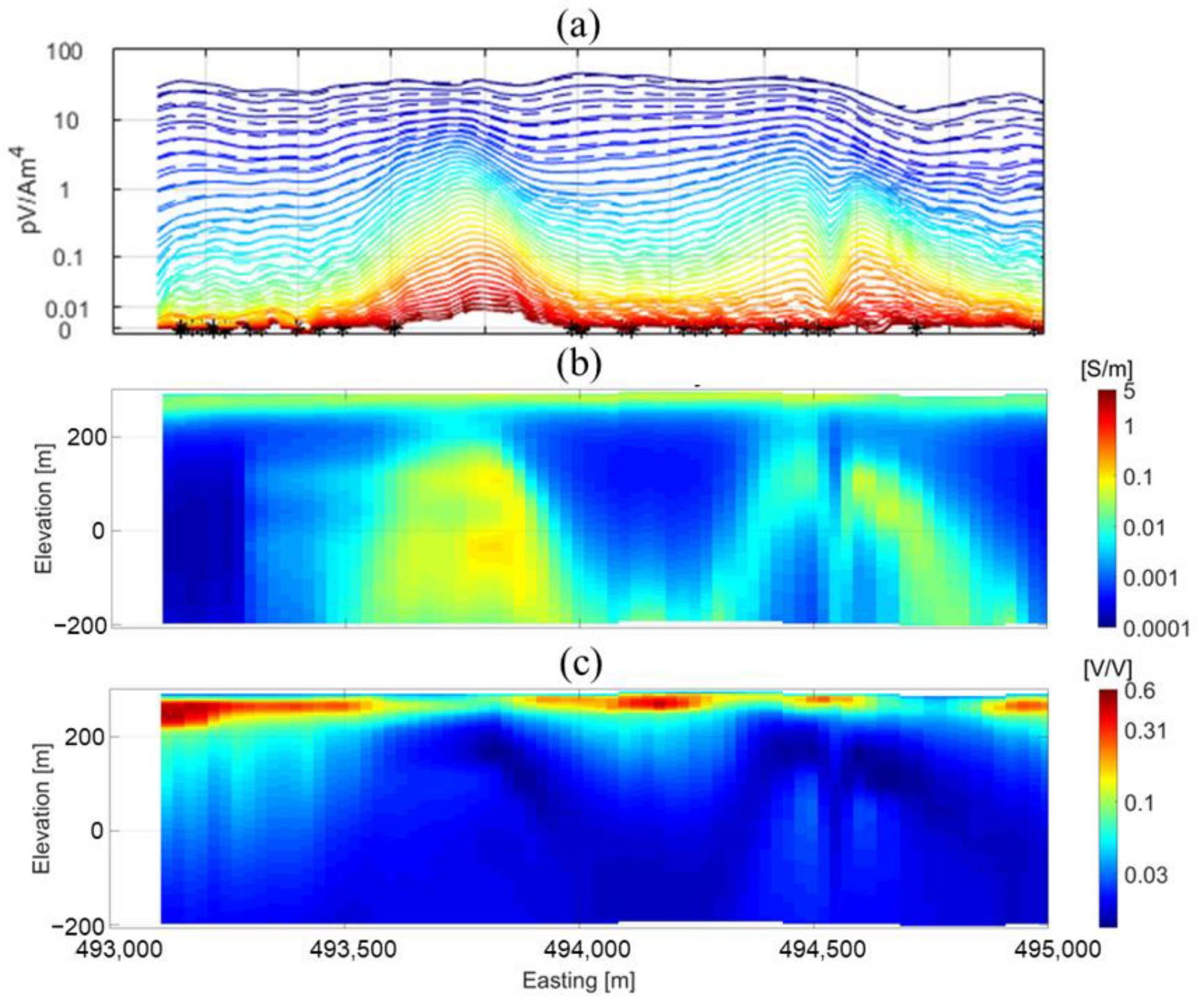
Figure 3 presents the results of the 1D inversion. For all inversions, the absolute error floors were set at 0.003 pV/Am4 for the vertical component and 0.01 pV/Am4 for the inline component (for 3D inversion only), and the percent error was set to 10% for both components (see Equation (2)). The conductive overburden is very well imaged in the 1D inversion. The instrument’s footprint is smaller near the Earth’s surface, and the overburden is relatively smooth laterally, which are ideal conditions for 1D inversion to operate. The chargeable overburden is also properly described.

Figure 3.
1D inversion results. The top panel (a) shows the observed data (solid lines) and predicted data (dotted lines) of the vertical component. The time channels extend from 41 μs (blue) to 8247 µs (red). Black asterisks show rejected data points. The second panel (b) shows the recovered conductivity model from the 1D inversion along the line 1060. The bottom panel (c) shows the recovered chargeability model from the 1D inversion along the line 1060. The data fit is for the model shown with the 1D approximation used for the forward modeling. It appears to be quite good but does not represent the true data fit, as evaluated by 3D modeling.
At depth, the blocky structure imaged to the west (left) of the image between 493,500 mE and 494,000 mE and starting around 200 m MSL (about 100 m below the Earth’s surface) does not have obvious artifacts from the 1D inversion. Subtle variations can be seen in the vertical component data over this conductor, indicative of lateral conductivity changes within this body, but the resolution using only the vertical component is limited. The conductive feature to the east centered slightly right of 494,500 mE is not imaged well in the 1D inversion. The experienced interpreter will recognize the classic “M” shape in the vertical component data, indicating an electrically thin conductor at depth with a null over the top of the conductor. This creates the obvious “pant leg” artifacts in the conductivity model with an apparent conductivity low where the conductor should be.
The data fit appears quite good after the 1D inversion, but in fact, it is not representative of the model shown because it was calculated for individual laterally invariant models for each observation point. To evaluate the true data fit, the synthetic data must be modeled in 3D, and the data fit must be calculated after this (see Figure 4).
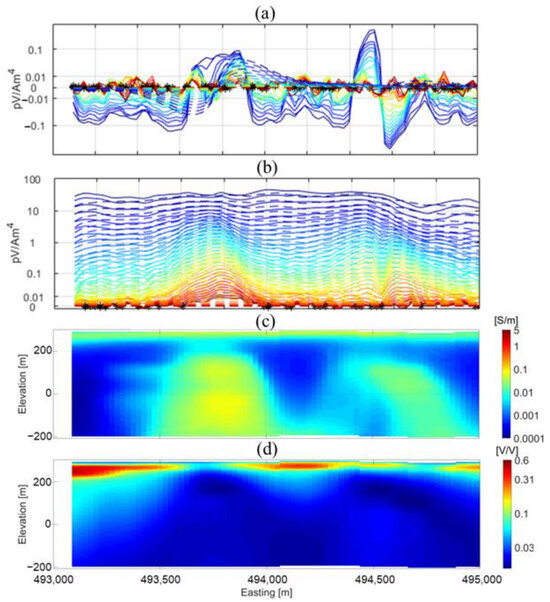
Figure 4.
Smoothed 1D inversion results used as input into the 3D inversion. The top panel (a) shows the observed data (solid lines) and predicted data (dotted lines) of the inline component modeled in full 3D. The time channels extend from 514 μs (blue) to 8247 µs (red). Black asterisks show rejected data points. The second panel (b) shows the observed data (solid lines) and predicted data (dotted lines) of the vertical component. The time channels extend from 41 μs (blue) to 8247 µs (red). The third panel (c) shows the smoothed 1D conductivity model used for the 3D inversion starting model. The bottom panel (d) shows the smoothed 1D chargeability model used for the 3D inversion starting model.
Figure 4 shows the smoothed model from the 1D inversion results. This is used as the starting and reference model for the 3D inversion. Comparing Figure 3 and Figure 4, note the conductors at depth have been smoothed and their artifacts reduced. The body on the left has undergone little change from the smoothing, as has the conductive overburden. The conductor showing the pant leg artifact has been smoothed into a coherent body and the center conductive low has been eliminated. As the initial model for the 3D inversion, this is first modeled with the 3D hybrid FD code to obtain residuals for inversion. Note the poor data fit after the 3D modeling based on the smoothed model from the 1D inversion results. The conductivity contrast of the conductive body on the left is dramatically underestimated, as shown by the poor late time data fit of the vertical component. There is no null in the vertical data component over the conductor on the right. The inline component is especially poorly fit. The positive-to-negative strong zero-crossing over the eastern anomaly shown in the observed data, which indicates a thin vertical conductor with vertically polarized current, is absent in the predicted response. The western anomaly has a reasonable fit in some areas but is not near the instrument’s noise level. In summary, 3D modeling based on the 1D inversion results does not generate predicted data that fit the observed data.
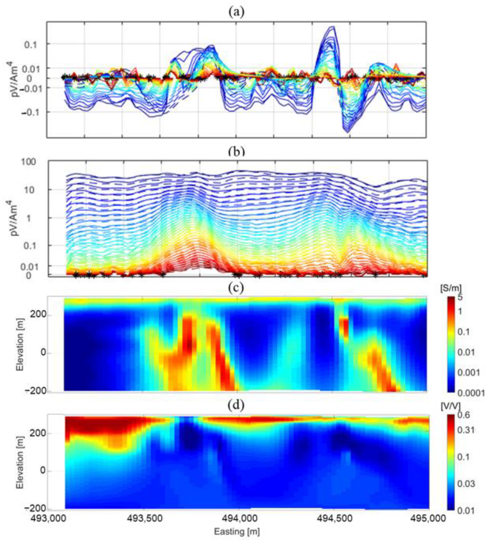
The last step is applying rigorous 3D inversion to the observed data using the smoothed model from the 1D inversion results as a starting model. In this case, the predicted data fit the observed data reasonably well (top panels in Figure 5). The bottom panels of Figure 5 show the vertical sections of 3D inversion results. One can see about 30 m of moderately (~30 Ohm-m) conductive overburden in the 3D model, which is retained from the 1D inversion results. The chargeability section also shows results that are very similar to the 1D inversion results, albeit with a slight thickening in the west (left). Below the overburden, the background conductivity of the model also does not change, with a largely nonpolarizable lower half-space of 1000 s Ohm-m.
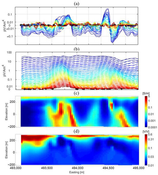
Figure 5.
Final 3D inversion results extracted from the line 1060 from the 3D model. The top panel (a) shows the observed data (solid lines) and predicted data (dotted lines) of the inline component modeled in full 3D. The time channels extend from 514 μs (blue) to 8247 µs (red). Black asterisks show rejected data points. The second panel (b) shows the observed data (solid lines) and predicted data (dotted lines) of the vertical component. The time channels extend from 41 μs (blue) to 8247 µs (red). The third panel (c) shows the final conductivity model extracted from the 3D inversion results. The fourth panel (d) shows the final chargeability model extracted from the 3D inversion results.
In the deeper sections, however, the resolution of the anomalies of interest is dramatically improved from the 1D model. The western anomaly is sharpened, the contrast increased ten times from 0.01–0.1 S/m to around 1 Ohm-m, and the anomaly is divided into two distinct parts. The eastern anomaly is now imaged in the correct location, with a thin vertical conductor under the null in the vertical component data. A second, deeper anomaly which dips steeply eastward is also imaged. Most importantly, the predicted data fit the observed data when modeled in 3D. It can be seen from the data that the inline component largely drives the lateral variations in the 3D inversion.
Figure 6 shows the recovered relaxation coefficient and time constant from the final 3D inversion. These parameters have better resolution in areas with strong chargeability, and poorer resolution in areas with weak chargeability. The near-surface chargeability anomaly shows relaxation coefficients of nearly 1, and the shortest time constants of around 4 × 10⁻⁵ s. These values likely indicate clays and near-surface regolith, which is appropriate given the geological setting. An obvious anomaly (0.65 []) in the relaxation coefficient is imaged around 100 m MSL and 494,500 mE, corresponding with the eastern conductive anomaly. More research is needed to explain and interpret these values fully.
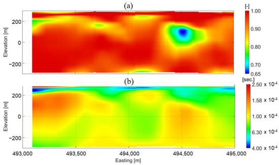
Figure 6.
Final 3D inversion results extracted from the line 1060 from the 3D model. The top panel (a) shows the recovered relaxation coefficient (C), and the bottom panel (b) shows the recovered time constant.
4. Discussion
The inverse problem of recovering conductivity models from time domain AEM data is an ill-posed problem, meaning that it is non-unique and unstable [32,35]. With the inclusion of the IP effect, up to three more unknown parameters (chargeability, time constant, relaxation coefficient) are added to the inverse problem, exacerbating the ill-posedness. Performing the inversion in 3D also expands the subset of models that will fit the data. In this case, including a polarizable model was required to fit the data to the noise level, with RMS values of only 1.5 being reached (instead of 1) when a non-polarizable conductivity was used. A 3D model was also required to fit the X component data and extract information from this component.
One-dimensional inversion, typically used because it simplifies the forward modeling and decreases computational time and memory requirements of inversion, is also a form a regularization. This helps to reduce the model space and non-uniqueness of the inversion. It also allows more efficient exploration of the 1D class of models, data error levels, and regional conductivity structures. Conductive overburden, layering, and regional background conductivities are well developed with the 1D model. There are two major drawbacks to the 1D inversion method: (1) no inline (or crossline) component data is used, which essentially ignores the half of the collected data that offers the best lateral resolution, and (2) a comparison of the synthesized data to the observed data is not a measure of the correctness of the model [17]. In other words, the data synthesized from the 1D inversion do not accurately represent the model portrayed as a stitched 3D section. Three-dimensional modeling must be performed to see an accurate representation of the stitched 3D model response.
The developed methodology builds the 3D conductivity and polarizable model in a series of steps, which optimize the use of apparent values and 1D inversions, then takes the final step of including inline data in the inversion. For example, in our case study, we believe the western anomaly would not be properly resolved with any method using only the vertical component of the data. Many local minimums in the model recovery process are avoided by starting with a smoothed model from 1D inversion. By virtue of the 3D modeling, the synthesized data can be used to evaluate the validity of the final recovered model. While the inversion attempts to fit all collected data within the noise level, deviations are often seen, such as near 493,700 mE in the late time inline component of the final inversion (Figure 5a). This allows quantitative evaluation of the developed model, and if the data do not fit adequately, one can perform additional inversions to fit the data better or at least realize that the model is incomplete.
5. Conclusions
We have developed a methodology that combines the advantages of several different AEM data interpretation techniques, from apparent parameters to 3D inversion, to build a comprehensive 3D model. The TargetEM system was shown to collect accurate multi-component data that can be used for quantitative inversion from 40 µs to 8.2 ms. The 3D inversion uses a hybrid 3D FD-IE scheme to rapidly and accurately model 3D data and compute sensitivities. All measured times and components are used in the workflow, as are the full physics, including induced polarization and three-dimensionality. The quality of the final model can be assessed using the data fit, even in complex areas with rapidly varying laterally conductivity and chargeability. Non-uniqueness states that fitting the observed data does not mean the model is correct. However, if the data are not fit, the model is most certainly incorrect. We should strive to honor all the collected data.
Author Contributions
Conceptualization, M.S.Z., L.H.C. and A.P.; methodology, M.S.Z., L.H.C. and A.P.; software, L.H.C.; validation, M.S.Z. and A.P.; formal analysis, M.S.Z., L.H.C. and A.P.; investigation, M.S.Z., L.H.C. and A.P.; resources, M.S.Z. and A.P.; data curation, A.P.; writing—original draft preparation, L.H.C.; writing—review and editing, L.H.C. and M.S.Z.; visualization, L.H.C.; supervision, M.S.Z.; project administration, M.S.Z.; funding acquisition, M.S.Z. and A.P. All authors have read and agreed to the published version of the manuscript.
Funding
This research was supported by TechnoImaging LLC and Expert Geophysics Ltd. and received no external funding.
Data Availability Statement
Data that support the findings of this study are available from the corresponding author upon reasonable request.
Acknowledgments
We acknowledge the support of TechnoImaging LLC, Expert Geophysics, Ltd., and CEMI, University of Utah.
Conflicts of Interest
Leif H. Cox was employed by TechnoImaging, and Alexander Prikhodko was employed by Expert Geophysics Limited. The remaining authors declare that the research was conducted in the absence of any commercial or financial relationships that could be construed as a potential conflict of interest.
References
- Flis, M.F.; Newman, G.A.; Hohmann, G.W. Induced-polarization effects in time-domain electromagnetic measurements. Geophysics 1989, 54, 514–523. [Google Scholar] [CrossRef]
- Smith, R.S.; West, G.F. Inductive interaction between polarizable conductors; an explanation of a negative coincident-loop transient electromagnetic response. Geophysics 1988, 53, 677–690. [Google Scholar] [CrossRef]
- Smith, R.S.; Klein, J. A special circumstance of airborne induced polarization measurements. Geophysics 1996, 61, 66–73. [Google Scholar] [CrossRef]
- Macnae, J.; Hine, K. Comparing induced polarization responses from airborne inductive and galvanic ground systems: Tasmania. Geophysics 2016, 81, E471–E479. [Google Scholar] [CrossRef]
- Viezzoli, A.; Kaminski, V. Airborne IP: Examples from the Mount Milligan Deposit, Canada, and the Amakinskaya Kimberlite Pipe, Russia. Explor. Geophys. 2016, 47, 269–278. [Google Scholar] [CrossRef]
- Lei, D.; Ren, H.; Fu, C.; Wang, Z.; Zhen, Q. Computation of analytical derivatives for Airborne TEM inversion using a Cole–Cole parameterization based on the current waveform of the transmitter. Sensors 2022, 23, 439. [Google Scholar] [CrossRef] [PubMed]
- Couto Junior, M.A.; Fiandaca, G.; Maurya, P.K.; Christiansen, A.V.; Porsani, J.L.; Auken, E. AEMIP robust inversion using maximum phase angle Cole–Cole model re-parameterisation applied for HTEM survey over Lamego gold mine, Quadrilátero Ferrífero, MG, Brazil. Explor. Geophys. 2020, 51, 170–183. [Google Scholar] [CrossRef]
- Kang, S.; Fournier, D.; Oldenburg, D.W. Inversion of airborne geophysics over the DO-27/DO-18 Kimberlites—Part 3: Induced polarization. Interpretation 2017, 5, T327–T340. [Google Scholar] [CrossRef]
- Viezzoli, A.; Manca, G. On airborne IP effects in standard AEM systems: Tightening model space with data space. Explor. Geophys. 2020, 51, 155–169. [Google Scholar] [CrossRef]
- Cox, L.H.; Zhdanov, M.S.; Pitcher, D.H.; Niemi, J. Three-dimensional inversion of induced polarization effects in airborne time domain electromagnetic data using the GEMTIP model. Minerals 2023, 13, 779. [Google Scholar] [CrossRef]
- Kwan, K.; Prikhodko, A.; Legault, J.M.; Plastow, G.; Xie, J.; Fisk, K. Airborne inductive induced polarization chargeability mapping of VTEM data. ASEG Ext. Abstr. 2015, 2015, ab104. [Google Scholar] [CrossRef]
- Chen, T.; Hodges, G.; Smiarowski, A. Extracting subtle IP responses from airborne time domain electromagnetic data. In Proceedings of the SEG International Exposition and Annual Meeting, SEG-2015-5828596, New Orleans, LA, USA, 18–23 October 2015. [Google Scholar]
- Macnae, J. Quantifying airborne induced polarization effects in helicopter time domain electromagnetics. J. Appl. Geophys. 2016, 135, 495–502. [Google Scholar] [CrossRef]
- Kai-Feng, M.; Chang-Chun, Y.; Yun-He, L.; Xiu-Yan, R.; Si-Yuan, S.; Jia-Jia, M.; Bin, X. Inversion of time-domain airborne EM data with IP effect based on Pearson correlation constraints. Appl. Geophys. 2020, 17, 589–600. [Google Scholar] [CrossRef]
- Di Massa, D.; Fedi, M.; Florio, G.; Vitale, A.; Viezzoli, A.; Kaminski, V. Joint interpretation of AEM and aeromagnetic data acquired over the Drybones Kimberlite, NWT (Canada). J. Appl. Geophys. 2018, 158, 48–56. [Google Scholar] [CrossRef]
- Fiandaca, G.; Auken, E.; Christiansen, A.V.; Gazoty, A. Time-domain-induced polarization: Full-decay forward modeling and 1D laterally constrained inversion of Cole–Cole parameters. Geophysics 2012, 77, E213–E225. [Google Scholar] [CrossRef]
- Ellis, R.G. Inversion of airborne electromagnetic data. Explor. Geophys. 1998, 29, 121–127. [Google Scholar] [CrossRef]
- Goold, J.W.; Cox, L.H.; Zhdanov, M.S. Spectral complex conductivity inversion of airborne electromagnetic data. In Proceedings of the SEG Technical Program Expanded Abstracts 2007, San Antonio, TX, USA, 23–28 September 2007; pp. 487–491. [Google Scholar]
- Kang, S.; Oldenburg, D.W. On recovering distributed IP information from inductive source time domain electromagnetic data. Geophys. J. Int. 2016, 207, 174–196. [Google Scholar] [CrossRef]
- Zhdanov, M. Generalized effective-medium theory of induced polarization. Geophysics 2008, 73, F197–F211. [Google Scholar] [CrossRef]
- Prikhodko, A.; Bagrianski, A.; Kuzmin, P.; Carpenter, A. Passive and active airborne electromagnetics -separate and combined technical solutions and applicability. In Proceedings of the ASEG Extended Abstracts; ASEG: Crows Nest, NSW, Australia, 2023; Volume 8. [Google Scholar]
- Raiche, A. Modelling the time-domain response of AEM systems. Explor. Geophys. 1998, 29, 103–106. [Google Scholar] [CrossRef]
- Pelton, W.H. Interpretation of Induced Polarization and Resistivity Data. Ph.D. Thesis, University of Utah, Salt Lake City, UT, USA, 1977. [Google Scholar]
- Zhdanov, M.S. Inverse Theory and Applications in Geophysics; Elsevier: Amsterdam, The Netherlands, 2015; Volume 36. [Google Scholar]
- Cox, L.H.; Wilson, G.A.; Zhdanov, M.S. 3D inversion of airborne electromagnetic data. Geophysics 2012, 77, WB59–WB69. [Google Scholar] [CrossRef]
- Nabighian, M.N. Electromagnetic Methods in Applied Geophysics: Voume 1, Theory; Society of Exploration Geophysicists: Houston, TX, USA, 1988; ISBN 0-931830-51-6. [Google Scholar]
- Viezzoli, A.; Christiansen, A.V.; Auken, E.; Sørensen, K. Quasi-3D modeling of airborne TEM data by spatially constrained inversion. Geophysics 2008, 73, F105–F113. [Google Scholar] [CrossRef]
- Cox, L.H.; Zhdanov, M.S. 3D Airborne electromagnetic inversion using a hybrid edge-based FE-IE method with moving sensitivity domain. In Proceedings of the SEG International Exposition and Annual Meeting, SEG-2014-0927, Denver, CO, USA, 26–31 October 2014. [Google Scholar]
- Yoon, D.; Zhdanov, M.S.; Mattsson, J.; Cai, H.; Gribenko, A. A hybrid finite-difference and integral-equation method for modeling and inversion of marine controlled-source electromagnetic data. Geophysics 2016, 81, E323–E336. [Google Scholar] [CrossRef]
- Newman, G.A.; Alumbaugh, D.L. Frequency-domain modelling of airborne electromagnetic responses using staggered finite differences. Geophys. Prospect. 1995, 43, 1021–1042. [Google Scholar] [CrossRef]
- Zhdanov, M.S. Geophysical Inverse Theory and Regularization Problems; Elsevier: Amsterdam, The Netherlands, 2002; Volume 36, ISBN 0-08-053250-0. [Google Scholar]
- Schenk, O.; Gärtner, K. PARDISO. In Encyclopedia of Parallel Computing; Padua, D., Ed.; Springer: Boston, MA, USA, 2011; pp. 1458–1464. ISBN 978-0-387-09766-4. [Google Scholar]
- Kaminski, V.; Prikhodko, A.; Oldenburg, D. Using ERA low frequency E-field profiling and UBC 3D frequency-domain inversion to delineate and discover a mineralized zone in Porcupine District, Ontario, Canada. In SEG Technical Program Expanded Abstracts 2011; Society of Exploration Geophysicists: Houston, TX, USA, 2011; pp. 1262–1266. ISBN 1052-3812. [Google Scholar]
- Poulsen, K.H. Geological classification of Canadian gold deposits. Bull. Geol. Surv. Can. 2000, 540, 1–106. [Google Scholar]
- Tikhonov, A.N.; Arsenin, V.I. Solutions of Ill-Posed Problems; Scripta Series in Mathematics; Halsted Press: Ultimo, Australia, 1977; ISBN 978-0-470-99124-4. [Google Scholar]


Disclaimer/Publisher’s Note: The statements, opinions and data contained in all publications are solely those of the individual author(s) and contributor(s) and not of MDPI and/or the editor(s). MDPI and/or the editor(s) disclaim responsibility for any injury to people or property resulting from any ideas, methods, instructions or products referred to in the content. |
© 2024 by the authors. Licensee MDPI, Basel, Switzerland. This article is an open access article distributed under the terms and conditions of the Creative Commons Attribution (CC BY) license (https://creativecommons.org/licenses/by/4.0/).