1. Introduction
The observed gravity and magnetic data offer crucial insights into geological makeup, particularly vital in exploring mineral resources. Challenges arise in conducting 3D inversions of regional gravity and magnetic data due to the considerable scale of the inversion area and the lack of a unique solution to the inverse problem. One strategy to mitigate this lack of uniqueness involves jointly inverting diverse physical field data, such as gravity and magnetics. Moreover, incorporating prior knowledge about the internal structure of the Earth’s crust can further narrow down the range of potential inverse models.
Over recent decades, the approach based on structure-coupled constraints was widely used in the joint inversion of multiphysics data (e.g., [
1,
2,
3,
4,
5,
6,
7,
8,
9,
10]). It is based on minimizing the value of the cross-gradients between different model parameters. This approach has been widely used for the joint inversion of geophysical data (e.g., [
11,
12,
13,
14]).
Another approach, utilizing Gramian constraints, was introduced in [
15]. The focus of this study is on the fundamentals of combined gravity and magnetic inversion for extensive datasets, utilizing Gramian constraints. Additionally, we outline a technique for integrating established basement depths into this joint inversion process. This developed methodology has been put into practice through a basement depth-guided joint inversion aimed at interpreting both the Bouguer gravity anomaly and the total magnetic intensity (TMI) anomaly observed in the vicinity of the Victoria Mine area in Nevada, USA (see
Figure 1).
The datasets containing observed gravity and magnetic data can be substantial due to the dense sampling that is common in contemporary airborne surveys. Processing such large datasets for inversion demands significant computer memory and efficient algorithms for accurate computations. This study employs inversion techniques utilizing point-mass approximation methods, significantly enhancing computational speed across all processes.
The U.S. Geological Survey (USGS) has been actively constructing a National Crustal Model for the continental United States [
16]. In previous publications, the basement depth was defined as “the depth to the uppermost surface of igneous or metamorphic rocks, with rocks above this depth comprising sediments or sedimentary rocks”. However, this definition lacked specificity in identifying the basement due to the possibility of sedimentary rocks undergoing metamorphism, resulting in a notable density increase. This study utilizes gravity and magnetic data to ascertain the depth at which a significant contrast in density and magnetization exists below the surface, which, in certain instances, might align with the boundary of the crystalline basement. Additionally, basement depth data can be derived through depth-to-basement inversion methods [
17,
18,
19,
20] and subsequently employed as a pre-existing model for inverting gravity and magnetic data.
To showcase our interpretation methodology, we opted to use gravity and total magnetic intensity (TMI) data extracted from the vicinity of Victoria Mine, Nevada. In
Figure 1, the highlighted red rectangular boundary delineates the designated area of interest (AOI). Spanning 100 km by 80 km, this AOI encompasses a total area of 8000 km
2. The corresponding gravity anomaly is visually represented in
Figure 2.
2. The Voxel-Based 3D Inversion with Regularization
Inverting potential field data poses a significant challenge due to its non-uniqueness, leading to potentially ambiguous interpretations. The application of regularization methods becomes essential to address the inherent complexity and ambiguity in the inverse problem [
21,
22,
23].
These methodologies play a critical role in alleviating the inherent ill-posed nature of the issue. The general formulation of the potential field inverse problem can be articulated as follows:
Here, m is a vector of model parameters (for a gravity inversion, , the density; for a magnetic inversion, , the susceptibility) of the order ; d is a vector of observed data (e.g., for gravity data; for magnetic TMI data) of the order , and is a forward modeling operator. In the case of gravity and magnetic fields, the forward modeling operator is a linear operator; then, is the matrix of this operator. In most cases of the 3D inversion of geophysical survey data, the size of vector of the model parameter, , is much larger than the size of vector d of the observed data, , that is, .
To tackle the inverse problem (1) and determine the model parameters represented by
, we adhere to the conventional structure of the regularization method. Solving the inverse problem (1) involves minimizing the associated parametric functional [
21,
22,
23]:
where
is the data weighting matrix;
is the a priori model; and
is a diagonal matrix of the model parameter weights based on integrated sensitivity:
where
is the Fréchet derivative matrix, and
when
is a linear operator.
This choice of model weights ensures an even sensitivity of the observed data to the model parameters situated across various depths and horizontal positions [
21,
22,
23].
Matrix
is a diagonal matrix of the minimum support stabilizing functional providing focusing inversion [
6]:
The minimization problem (2) is addressed utilizing the re-weighted regularized conjugate gradient (RRCG) technique, extensively elaborated upon in [
21,
22,
23].
3. Three-Dimensional Joint Inversion of Gravity and TMI Data
When performing a joint inversion of gravity and magnetic field data, the parametric functional (2) needs adjustment to encompass both gravity and magnetic misfit functionals. Additionally, a Gramian stabilizer is integrated to promote interaction between the density and magnetic inverse models [
24]:
where
is the observed gravity data and
is the observed magnetic data.
and
are the gravity and magnetic forward modeling operators (for details, see [
23,
25,
26]). The coefficients
and
are the weighting coefficients to balance the stabilizers of density and magnetization models. Parameters
,
and
β are the regularization parameters.
,
, and
are also defined based on the corresponding Fréchet matrices of operators
or
.
The term
is a Gramian stabilizer:
where (…,…) stands for the inner product between the corresponding model parameters [
23].
The Gramian stabilizer ensures a correlation between the density and magnetization inverse models, thereby guaranteeing geological consistency across both models [
23,
24].
4. Geology of the Victoria Copper Mine Area, Nevada
Nevada’s geological history was shaped by the collision and subsequent stretching of tectonic plates. This tectonic activity, along with the rain shadow effect caused by plate movements, transformed Nevada into a desert experiencing occasional significant floods. The state is characterized by rivers that predominantly flow into internal basins rather than towards the ocean. Ranking as the third most earthquake-prone state in the US, Nevada’s landscape is predominantly covered by volcanic rocks, notably observed at Yucca Mountain, the proposed site for a high-level radioactive waste repository. The towering mountains in the eastern part of the state preserve fossils that originated in an ancient ocean. Additionally, the valleys of Western Nevada were inundated by a much more recent Ice Age Lake.
The East Humboldt Range in the Northeast harbors Nevada’s oldest rocks, dating back around 2.5 billion years, indicated by a lead isotope analysis marking the boundary between the Archean and Proterozoic periods. Approximately 1.7 billion years ago, Clark County and the densely populated zones around Las Vegas were underlain by metamorphic and igneous rocks. Around one billion years ago, this area was positioned at the equator as part of the supercontinent Rodinia.
Between 700 and 600 million years ago, the continent experienced a rift, leading to the absence of continental rocks in western Nevada beyond the 700-million-year mark. This absence is attributed to the western portion of the region separating and merging with what is now modern-day Siberia [
27,
28,
29,
30].
The Victoria Copper Mine, situated near Currie, Nevada, has historically been a part of the Dolly Varden Mining District, first discovered back in 1872. Operating both as a surface and underground mining facility, it commenced initial production during the same year of its discovery. The mining operations predominantly involve underground workings, with a recorded mine capacity of 907 metric tons of ore per day in 1973, boasting a production unit cost of USD 10.55 per metric ton of ore. The mined ore comprises limonite, azurite, and chalcopyrite, while waste materials primarily consist of calcite, pyrite, and jasper. Information dating back to 1991 depicted the ore body’s shape and dimensions as unknown. The geological formations in this vicinity include quartz monzonite ranging from the Jurassic period (201.30 to 145.00 million years ago) to the Cretaceous period (145 to 66 million years ago) [
31].
The copper ore deposit at the Victoria mine is situated within a breccia pipe that intrudes Permian limestone and calcareous sandstone. The mineralized section of the breccia seems to result from a collapse. In other areas, the breccia comprises a mixture of various rock types within a matrix of finely ground rock particles, sometimes displaying rounded clasts and sporadic graded bedding, suggesting upward streaming as the emplacement mechanism. During brecciation, monzonite porphyry dikes infiltrated the pipe. Zonation and mineral development in the district and downward within the pipe progress from limestone to talc- and tremolite-bearing assemblages, further to diopside, and eventually to garnet (averaging 77% andradite). Brecciation occurred intermittently during silication: tremolite clasts were bound by diopside; diopside hornfels clasts were cemented initially by coarser diopside, then by diopside and calcite, marking the cessation of brecciation. Ultimately, garnet, calcite, quartz, and sulfide ore sealed the breccia. Copper accumulation primarily resides in a curved zone at one end of the breccia pipe. A subsequent alteration of diopside led to the development of saponite, talc, and localized serpentine, while garnet underwent transformation into mixtures of hematite, calcite, quartz, and chlorite. This sequence is categorized into three stages: (1) early contact metamorphism, (2) primary iron metasomatism alongside copper deposition, and (3) late-stage alteration, almost isochemical except for the introduction of CO
2 and H
2O [
31,
32].
5. Inversion of Bouguer Gravity Anomaly in the Area of Victoria Mine, Nevada
Gravity data encompassing the entirety of Nevada and neighboring regions of California, Utah, and Arizona were collated, comprising around 80,000 gravity stations primarily sourced from the National Geophysical Data Center and the U.S. Geological Survey. These gravity measurements were standardized to the Geodetic Reference System of 1967 and aligned with the Gravity Standardization Net 1971 gravity datum. The dataset underwent processing to derive complete Bouguer and isostatic gravity anomalies, involving the application of standard gravity adjustments, including terrain and isostatic corrections (refer to
Figure 2) (source:
https://pubs.usgs.gov/ds/2006/234/) (accessed on 5 January 2023).
At Victoria Mine in Nevada, the US Geological Survey (USGS) has identified a notably distinct density contrast surface linked to the Mesozoic basement. This depth-to-basement model serves as a flexible guideline within the inversion process.
Figure 3 showcases an illustration of the density contrast surface generated by the USGS [
16,
33].
We utilized the 3D inversion technique on the chosen Bouguer gravity anomaly within the Victoria Mine area of Nevada (as depicted in
Figure 2). The specific area subjected to inversion is delineated by a red rectangle, also visible in
Figure 1.
We utilized standard 3D voxel-type inversion on the filtered complete Bouguer gravity anomaly, as illustrated in
Figure 2. The filtering was carried out by a simple linear regional field removal to separate the anomalous field. The a priori model introduced in Equation (2) of the parametric functional was crafted using the density contrast surface exhibited in
Figure 3, featuring a relatively modest contrast of 0.05 g/cc. The 3D inversion domain was discretized into 84 × 104 × 20 = 174,720 rectangular cells. For comparative analysis, we conducted inversions both with and without the a priori density contrast model. In both scenarios, we employed the iterative re-weighted regularized conjugate gradient (RRCG) method until the discrepancy between the observed and predicted data reached a 5% threshold.
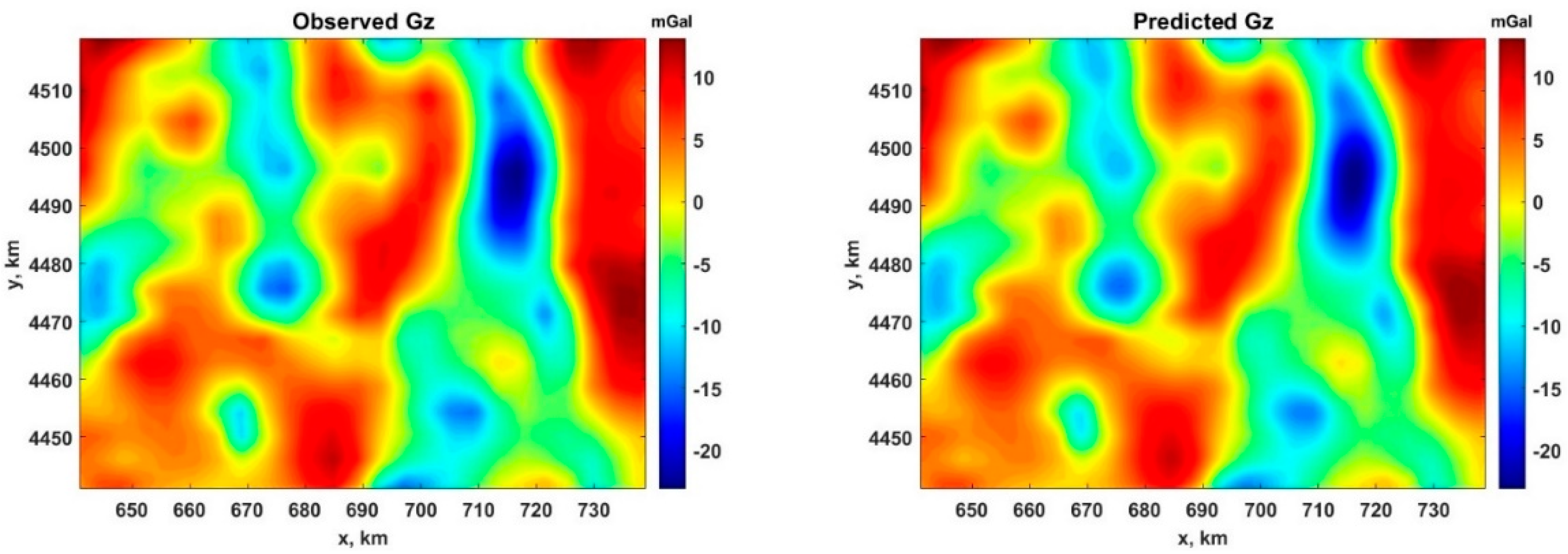
Figure 4 and
Figure 5 correspondingly display the observed and predicted gravity data resulting from the 3D inversions performed with and without the a priori density contrast model. It is evident that both inversion approaches effectively replicate the observed data.
We conducted an analysis and comparison of the 3D density models generated by the two inversion methods.
Figure 6 shows the location of selected profiles over the gravity data.
Figure 7 and
Figure 8 depict vertical sections along profiles AA’, BB’, and CC’, showcasing the 3D density models derived from the inversion without and with the a priori density contrast model.
Incorporating the a priori density contrast model into the solution for the inverse problem yields a precise demarcation of the base of the unconsolidated sediments and the basement’s upper boundary. Simultaneously, our inverse density model aligns effectively with the depth model indicated by the dashed lines in
Figure 3. This demonstrates the capability of guided inversion to refine the a priori model for a better fit with the observed data—a data-driven approach, essentially. We should also note the difference in results concerning the mine area. The density anomaly under the mine is at the surface in the unconstrained models. In the constrained model, the density anomaly is buried as we move away from the mine.
6. Inversion of TMI Anomaly in the Area of Victoria Mine, Nevada
The magnetic data over Nevada are part of digital data grids for the magnetic anomaly map of North America, the new digital magnetic anomaly database and map of North America (usgs.gov) (
https://pubs.usgs.gov/of/2002/ofr-02-414/) (accessed on 5 January 2023).
The collaborative efforts of the Geological Survey of Canada (GSC), the U.S. Geological Survey (USGS), and the Consejo de Recursos Minerales of Mexico (CRM) produced the digital magnetic anomaly database and map for the North American continent. This modern, integrated digital repository of magnetic anomaly data serves as a valuable resource, easily accessible and equipped to aid in further examining the continent’s structure, geological processes, and tectonic evolution. Moreover, it has the potential to contribute to resolving societal and scientific issues that transcend national borders. The North American magnetic anomaly map, derived from this digital database, offers a comprehensive magnetic perspective encompassing continental-scale patterns not found in individual datasets. It plays a crucial role in connecting widely separated geological outcrop areas and harmonizing diverse geological investigations.
The data grids are set with a 1 km interval and are mapped onto the DNAG projection (a spherical transverse Mercator projection), centered at a central meridian of 100° W, base latitude of 0°, employing a scale factor of 0.926, and an Earth radius of 6,371,204 m. These grids specifically represent the magnetic field at an altitude of 305 m above the terrain, subsequently realigned to the original 1 km grid [
34,
35,
36].
In Nevada, the US Geological Survey (USGS) identified a notably distinct depth to the basement surface linked to the Mesozoic basement [
33]. This basement model serves as a guiding reference in our inversion process. We implement a voxel-type 3D susceptibility inversion technique, incorporating the depth-to-basement model (refer to
Figure 3) as a flexible constraint within the inversion process.
The TMI anomaly region chosen for inversion was specifically picked around Victoria Mine, Nevada, as indicated in
Figure 1 and
Figure 9. In
Figure 9, a red rectangle in the map’s northeast marks the designated area of interest (AOI).
For the magnetic field data inversion, we utilized the depth-to-basement model displayed in
Figure 3 as prior information, maintaining a susceptibility contrast of 0.003. This specific value was established through a consideration of existing data and ensured the optimal convergence of the inversion process. The iterative inversion procedure continued until the L2 misfit, indicating the disparity between observed and predicted data, reaching approximately 3%.
Subsequently, we employed a standard 3D volume integral approach to invert the TMI anomaly, filtering it through a basic plane removal process (refer to
Figure 9). The 3D inversion space was divided into a grid of 84 × 104 × 20 = 174,720 rectangular cells. For this phase, we conducted inversions both with and without the a priori model.
Figure 10 and
Figure 11 illustrate that both inversion methods effectively replicate the observed data.
Selected profiles are shown in
Figure 12 overlying the TMI data. It is intriguing to compare the 3D susceptibility models generated by two inversion methods. For instance, in
Figure 13 and
Figure 14, we present vertical cross-sections along profiles AA’, BB’, and CC’, showcasing the 3D susceptibility models obtained from inversions, both with and without incorporating the a priori basement model. These visuals highlight that integrating the a priori basement model into the inverse problem solution enhances our capability to define the lower boundary of loose sediments and the upper limit of the basement more accurately. Moreover, the resulting inverse susceptibility model aligns well with depth, signifying the guided inversion’s capacity to refine the a priori model to better fit the observed data. In essence, this guided inversion embodies a data-centric approach.
7. Joint Inversion of Gravity and Magnetic Data Selected in the Area of the Victoria Mine, Nevada
To conclude, we performed a joint inversion of gravity and magnetic data within the Victoria Mine area in Nevada, as illustrated in
Figure 2 and
Figure 9. The 3D joint inversion space was subdivided into 84 × 104 × 20 = 174,720 rectangular cells. In this phase, the joint inversion was executed while incorporating the a priori model. Specifically, we utilized a density contrast surface, depicted in
Figure 3, characterized by a relatively modest density contrast of 0.05 g/cc and a susceptibility contrast of 0.003, as the basis for the a priori model. Throughout the iterative inversions, we achieved an L2 misfit between observed and predicted data, maintaining a level of less than 5% for gravity inversion and 3% for magnetic inversion.
The parameters in Equation (5) for the parametric functional were selected as follows:
where
is the iteration number.
Figure 15 shows that both gravity and magnetic data predicted by joint inversions reproduce the observed data well.
Figure 16 and
Figure 17 display vertical cross-sections of gravity density and magnetic susceptibility models along profiles AA’, BB’, and CC’, respectively. These visuals demonstrate that integrating the a priori basement model into the joint inverse problem solution allows for a clear delineation of the lower boundary of unconsolidated sediments and the upper limit of the basement. Additionally, the resulting inverse density and susceptibility models align well with depth. This underscores the guided joint inversion’s capability to refine the a priori model effectively, ensuring a proper fit with the observed data.
In addition,
Figure 16 shows the density anomaly in the joint inverted density model directly east of the mine. This was not present in the separate gravity data inversion (
Figure 8). Thus, the resulting 3D density and susceptibility model specific to the Victoria Mine area in Nevada offers crucial insights into the intricate geological composition of the region and provides details regarding the thickness of unconsolidated sediments.
8. Conclusions
Gravity and magnetic surveys are powerful tools for conducting extensive regional geological investigations of the Earth’s crust. They provide valuable insights into the distribution of density and susceptibility within sediment layers and the crystalline basement. In certain exploration areas, prior knowledge of the depth-to-basement may be available through borehole data or seismic information. This depth information can be used as a flexible constraint in traditional 3D volume inversions, helping to address the challenges of non-uniqueness and instability often encountered in solving inverse problems.
Our research demonstrates how joint inversion with Gramian constraints can effectively reduce the inherent ambiguity in potential field inversions. This approach ultimately enhances confidence in the reconstructed geological structure within the surveyed area.
We applied the refined constrained joint inversion method to gravity and total magnetic intensity (TMI) anomaly data within the Victoria Mine area in Nevada. This joint inversion resulted in one of the initial 3D models of the upper crust within this region, providing detailed information about the distribution of density and susceptibility in the upper layers of the Earth’s crust at Victoria Mine, Nevada. Specifically, the zone immediately east of Victoria Mine exhibits high susceptibility and density relative to the surrounding area, suggesting a promising exploration target. These coincident anomalies near the mine are only evident in the joint inversion with the basement constraint, thus demonstrating that the method can provide unique geological insights in the area.
Author Contributions
Conceptualization, M.S.Z.; funding acquisition, M.S.Z.; software, M.J. and M.S.Z.; methodology, M.S.Z. and M.J.; validation, M.S.Z., L.W. and M.J.; investigation, M.S.Z., L.W. and M.J.; writing, M.S.Z., M.J. and L.W.; visualization, L.W.; supervision, M.S.Z. All authors have read and agreed to the published version of the manuscript.
Funding
This research was supported by CEMI and TechnoImaging and received no external funding.
Data Availability Statement
The data used in this study are publicly available from the United States Geological Survey (USGS).
Acknowledgments
We acknowledge the support of the Consortium for Electromagnetic Modeling and Inversion (CEMI) at the University of Utah, as well as TechnoImaging.
Conflicts of Interest
Michael S. Zhdanov, Le Wan, and Michael Jorgensen are the employees of TechnoImaging, LLC. The paper reflects the views of the scientists and not the company.
References
- Fregoso, E.; Gallardo, L.A. Cross-Gradients Joint 3D Inversion with Applications to Gravity and Magnetic Data. Geophysics 2009, 74, L31–L42. [Google Scholar] [CrossRef]
- Gallardo, L.A. Multiple Cross-Gradient Joint Inversion for Geospectral Imaging. Geophys. Res. Lett. 2007, 34, L19301. [Google Scholar] [CrossRef]
- Gallardo, L.A.; Meju, M.A. Characterization of Heterogeneous Near-Surface Materials by Joint 2D Inversion of DC Resistivity and Seismic Data. Geophys. Res. Lett. 2003, 30, 1658. [Google Scholar] [CrossRef]
- Gallardo, L.A.; Meju, M.A. Joint Two-Dimensional DC Resistivity and Seismic Travel-Time Inversion with Cross-Gradients Constraints. J. Geophys. Res. 2004, 109, B03311. [Google Scholar] [CrossRef]
- Gallardo, L.A.; Meju, M.A. Joint Two-Dimensional Cross-Gradient Imaging of Magnetotelluric and Seismic Traveltime Data for Structural and Lithological Classification. Geophys. J. Int. 2007, 169, 1261–1272. [Google Scholar] [CrossRef]
- Gallardo, L.A.; Meju, M.A. Structure-Coupled Multi-Physics Imaging in Geophysical Sciences. Rev. Geophys. 2011, 49, RG1003. [Google Scholar] [CrossRef]
- Haber, E.; Oldenburg, D. Joint Inversion: A Structural Approach. Inverse Probl. 1997, 13, 63–77. [Google Scholar] [CrossRef]
- Haber, E.; Modersitzki, J. Intensity Gradient Based Registration and Fusion of Multi-Modal Images. Methods Inf. Med. 2018, 46, 292–299. [Google Scholar] [CrossRef]
- Hu, W.; Abubakar, A.; Habashy, T.M. Joint Electromagnetic and Seismic Inversion Using Structural Constraints. Geophysics 2009, 74, R99–R109. [Google Scholar] [CrossRef]
- Li, X.; Li, Y.; Meng, X.; Meju, M.A. Joint Multi-Geophysical Inversion: Effective Model Integration, Challenges and Directions for Future Research. In Proceedings of the International Workshop on Gravity, Electrical & Magnetic Methods and Their Applications, Beijing, China, 10–13 October 2011; Li, X., Li., Y., Meng, X., Eds.; SEG Global Meeting Abstracts; Society of Exploration Geophysicists: Houston, TX, USA, 2011; p. 37. ISBN 978-1-56080-309-6. [Google Scholar]
- Colombo, D.; De Stefano, M. Geophysical Modeling via Simultaneous Joint Inversion of Seismic, Gravity, and Electromagnetic Data: Application to Prestack Depth Imaging. Lead. Edge 2007, 26, 326–331. [Google Scholar] [CrossRef]
- Jegen, M.D.; Hobbs, R.W.; Tarits, P.; Chave, A. Joint Inversion of Marine Magnetotelluric and Gravity Data Incorporating Seismic Constraints: Preliminary Results of Sub-Basalt Imaging off the Faroe Shelf. Earth Planet. Sci. Lett. 2009, 282, 47–55. [Google Scholar] [CrossRef]
- DeStefano, M.; Andreasi, F.G.; Re, S.; Virgilio, M.; Snyder, F.F. Multiple-Domain, Simultaneous Joint Inversion of Geophysical Data with Application to Subsalt Imaging. Geophysics 2011, 76, R69–R80. [Google Scholar] [CrossRef]
- Moorkamp, M.; Heincke, B.; Jegen, M.; Robert, A.W.; Hobbs, R.W. A Framework for 3-D Joint Inversion of MT, Gravity and Seismic Refraction Data. Geophys. J. Int. 2011, 184, 477–493. [Google Scholar] [CrossRef]
- Zhdanov, M.S.; Gribenko, A.V.; Wilson, G. Generalized Joint Inversion of Multimodal Geophysical Data Using Gramian Constraints. Geophys. Res. Lett. 2012, 39, L09301. [Google Scholar] [CrossRef]
- Shah, A.K.; Boyd, O.S.; Sowers, T.; Thompson, E. Building a USGS National Crustal Model: Theoretical Foundation, Inputs, and Calibration for the Western United States. In Proceedings of the AGU Fall Meeting Abstracts, New Orleans, LA, USA, 1 December 2017; Volume 2017, p. S53A-0654. [Google Scholar]
- Cai, H.; Zhdanov, M. Application of Cauchy-Type Integrals in Developing Effective Methods for Depth-to-Basement Inversion of Gravity and Gravity Gradiometry Data. Geophysics 2015, 80, G81–G94. [Google Scholar] [CrossRef]
- Zhdanov, M.S. Use of Cauchy Integral Analogs in the Geopotential Field Theory. Ann. Geophys. 1980, 36, 447–458. [Google Scholar]
- Zhdanov, M.S. Integral Transforms in Geophysics; Springer: Berlin/Heidelberg, Germany, 1988. [Google Scholar]
- Zhdanov, M.S.; Liu, X. 3-D Cauchy-Type Integrals for Terrain Correction of Gravity and Gravity Gradiometry Data. Geophys. J. Int. 2013, 194, 249–268. [Google Scholar] [CrossRef]
- Zhdanov, M.S. Geophysical Inverse Theory and Regularization Problems; Elsevier: Amsterdam, The Netherlands, 2002. [Google Scholar]
- Zhdanov, M.S. New Advances in Regularized Inversion of Gravity and Electromagnetic Data. Geophys. Prospect. 2009, 57, 463–478. [Google Scholar] [CrossRef]
- Zhdanov, M.S. Inverse Theory and Applications in Geophysics; Elsevier: Amsterdam, The Netherlands, 2015. [Google Scholar]
- Zhdanov, M.S.; Jorgensen, M.; Cox, L. Advanced Methods of Joint Inversion of Multiphysics Data for Mineral Exploration. Geosciences 2021, 11, 262. [Google Scholar] [CrossRef]
- Zhdanov, M.S.; Jorgensen, M.; Wan, L. Two-Step Approach to 3D Gravity Inversion: Case Study in the State of Utah. In Proceedings of the First International Meeting for Applied Geoscience & Energy Expanded Abstracts, Denver, CO, USA, 27–30 September 2021; SEG Technical Program Expanded Abstracts; Society of Exploration Geophysicists: Houston, TX, USA, 2021; pp. 916–920. [Google Scholar]
- Zhdanov, M.S.; Jorgensen, M.; Wan, L. Three-Dimensional Gravity Inversion in the Presence of the Sediment-Basement Interface: A Case Study in Utah, USA. Minerals 2022, 12, 448. [Google Scholar] [CrossRef]
- Lush, A.P.; McGrew, A.J.; Snoke, A.W.; Wright, J.E. Allochthonous Archean Basement in the Northern East Humboldt Range, Nevada. Geology 1988, 16, 349–353. [Google Scholar] [CrossRef]
- Price, J.G. The Geology of Nevada. Prof. Geol. 2002, 39, 2–8. [Google Scholar]
- Price, J.G.; Henry, C.D.; Castor, S.B.; Garside, L.; Faulds, J.E. Geology of Nevada with Excellent Rock Exposures in the Desert, Generally Good Access to Collecting Localities on Public Lands, and Fine Tourist Attractions in the Towns, Nevada Is a Wonderful State for Rock and Mineral Enthusiasts. Rocks Miner. 1999, 74, 357–363. [Google Scholar] [CrossRef]
- Price, J.G.; Meeuwig, R.O.; Tingley, J.V.; La Pointe, D.D.; Castor, S.B.; Davis, D.A.; Hess, R.H. The Nevada Mineral Industry-2001. In Nevada Bureau of Mines and Geology Special Publication MI-2001; NBMG Publications: Reno, NV, USA, 2002; pp. 3–12. [Google Scholar]
- Atkinson, W.W.; Kaczmarowski, J.H.; Erickson, A.J. Geology of a Skarn-Breccia Orebody at the Victoria Mine, Elko County, Nevada. Econ. Geol. 1982, 77, 899–918. [Google Scholar] [CrossRef]
- Cashion, W.B. Geology and Fuel Resources of the Green River Formation, Southeastern Uinta Basin, Utah and Colorado. U.S. Geol. Surv. Prof. Pap. 1967, 548. [Google Scholar] [CrossRef]
- Shah, A.K.; Boyd, O.S. Depth to Basement and Thickness of Unconsolidated Sediments for the Western United States—Initial Estimates for Layers of the U.S. Geological Survey National Crustal Model; Open-File Report; U.S. Geological Survey: Reston, VA, USA, 2018. [Google Scholar]
- Maus, S.; Rother, M.; Holme, R.; Lühr, H.; Olsen, N.; Haak, V. First Scalar Magnetic Anomaly Map from CHAMP Satellite Data Indicates Weak Lithospheric Field. Geophys. Res. Lett. 2002, 29, 4506–4513. [Google Scholar] [CrossRef]
- Ravat, D.; Whaler, K.A.; Pilkington, M.; Sabaka, T.; Purucker, M. Compatibility of High-Altitude Aeromagnetic and Satellite-Altitude Magnetic Anomalies over Canada. Geophysics 2002, 67, 546–554. [Google Scholar] [CrossRef]
- US Magnetic Anomaly Data Task Group. Rationale and Operational Plan to Upgrade the US Magnetic Anomaly Data Base; Task Group: Dallas, TX, USA, 1994. [Google Scholar]
Figure 1.
Red square is AOI on the topography map of Nevada (left panel). Red square is AOI on the geological map of Nevada (right panel).
Figure 1.
Red square is AOI on the topography map of Nevada (left panel). Red square is AOI on the geological map of Nevada (right panel).
Figure 2.
Nevada complete Bouguer gravity anomaly map over Nevada State (data from USGS
https://pubs.usgs.gov/ds/2006/234/data/) (accessed on 5 January 2023). The red square shown in the center of the map outlines the area of interest (AOI). The zoomed section has a different color scale to highlight local variations in the magnetic field.
Figure 3.
Map of the depth-to-the-basement (density contrast surface) produced by the USGS [
33].
Figure 3.
Map of the depth-to-the-basement (density contrast surface) produced by the USGS [
33].
Figure 4.
Comparison of the observed (left panel) and predicted (right panel) gravity data produced by 3D inversion with no a priori model.
Figure 4.
Comparison of the observed (left panel) and predicted (right panel) gravity data produced by 3D inversion with no a priori model.
Figure 5.
Comparison of the observed (left panel) and predicted (right panel) gravity data produced by 3D inversion with a priori density contrast model.
Figure 5.
Comparison of the observed (left panel) and predicted (right panel) gravity data produced by 3D inversion with a priori density contrast model.
Figure 6.
Filtered Bouguer gravity anomaly map. Red lines are the profiles AA’, BB’ and CC’ that are used in constructing the vertical sections of the density model produced by inversion.
Figure 6.
Filtered Bouguer gravity anomaly map. Red lines are the profiles AA’, BB’ and CC’ that are used in constructing the vertical sections of the density model produced by inversion.
Figure 7.
Vertical sections along profiles AA′, BB′, and CC′ of the 3D density model produced by the inversion without a priori model.
Figure 7.
Vertical sections along profiles AA′, BB′, and CC′ of the 3D density model produced by the inversion without a priori model.
Figure 8.
Vertical sections along profiles AA’, BB’, and CC’ of the 3D density model produced by the inversion with a priori density contrast model. The dashed line represents the surface of the basement model.
Figure 8.
Vertical sections along profiles AA’, BB’, and CC’ of the 3D density model produced by the inversion with a priori density contrast model. The dashed line represents the surface of the basement model.
Figure 9.
Filtered TMI anomaly map of Nevada (left panel). The red rectangle in the map (left panel) outlines the area of interest (AOI) presented in the right panel.
Figure 9.
Filtered TMI anomaly map of Nevada (left panel). The red rectangle in the map (left panel) outlines the area of interest (AOI) presented in the right panel.
Figure 10.
Comparison of the observed (left panel) and predicted (right panel) TMI data produced by 3D inversion without a priori model.
Figure 10.
Comparison of the observed (left panel) and predicted (right panel) TMI data produced by 3D inversion without a priori model.
Figure 11.
Comparison of the observed (left panel) and predicted (right panel) TMI data produced by 3D inversion with a priori basement model.
Figure 11.
Comparison of the observed (left panel) and predicted (right panel) TMI data produced by 3D inversion with a priori basement model.
Figure 12.
Filtered TMI anomaly map of the AOI. The horizontal red lines show the profiles AA’, BB’ and CC’ used in constructing the vertical sections of the susceptibility model produced by inversion.
Figure 12.
Filtered TMI anomaly map of the AOI. The horizontal red lines show the profiles AA’, BB’ and CC’ used in constructing the vertical sections of the susceptibility model produced by inversion.
Figure 13.
Vertical section along profiles AA’, BB’, and CC’ of 3D susceptibility model produced by the inversion without a priori model.
Figure 13.
Vertical section along profiles AA’, BB’, and CC’ of 3D susceptibility model produced by the inversion without a priori model.
Figure 14.
Vertical section along profiles AA’, BB’, and CC’ of 3D susceptibility model produced by the inversion with a priori basement model. The black dashed line represents the surface of the basement model.
Figure 14.
Vertical section along profiles AA’, BB’, and CC’ of 3D susceptibility model produced by the inversion with a priori basement model. The black dashed line represents the surface of the basement model.
Figure 15.
Comparison of the observed (left panel) and predicted (right panel) gravity and magnetic data produced by 3D joint inversion with a priori density contrast model.
Figure 15.
Comparison of the observed (left panel) and predicted (right panel) gravity and magnetic data produced by 3D joint inversion with a priori density contrast model.
Figure 16.
Vertical sections along profiles AA’, BB’, and CC’ of the 3D density model produced by the joint inversion with a priori density contrast model. The black dashed line represents the surface of the a priori basement model.
Figure 16.
Vertical sections along profiles AA’, BB’, and CC’ of the 3D density model produced by the joint inversion with a priori density contrast model. The black dashed line represents the surface of the a priori basement model.
Figure 17.
Vertical sections along profiles AA’, BB’, and CC’ of 3D susceptibility model produced by the joint inversion with a priori basement model. The black dashed line represents the surface of the basement model.
Figure 17.
Vertical sections along profiles AA’, BB’, and CC’ of 3D susceptibility model produced by the joint inversion with a priori basement model. The black dashed line represents the surface of the basement model.
| Disclaimer/Publisher’s Note: The statements, opinions and data contained in all publications are solely those of the individual author(s) and contributor(s) and not of MDPI and/or the editor(s). MDPI and/or the editor(s) disclaim responsibility for any injury to people or property resulting from any ideas, methods, instructions or products referred to in the content. |
© 2024 by the authors. Licensee MDPI, Basel, Switzerland. This article is an open access article distributed under the terms and conditions of the Creative Commons Attribution (CC BY) license (https://creativecommons.org/licenses/by/4.0/).


