Abstract
This work aimed to understand the relationships between grinding variables and the P80 (80% passing size) of a grinding circuit (feed to flotation). Canadian Royalties want to obtain and reduce variations in the P80, which is currently 65 micrometres. Thus, principal component analysis (PCA), part of machine learning, was utilized to better understand the factors that significantly influence the P80. PCA is meant to be used as a guideline for plant metallurgists to determine how the grinding circuit factors influence P80; thus, the variables can be manipulated to lower P80 fluctuations. PCA revealed that the head grade of the ore (pentlandite (Pn), chalcopyrite (Cp), pyrrhotite (Po) and non-sulphide gangue (NSG)) and the primary ball mill power were weakly correlated with P80. However, the ore level in the silo, flowrate to cyclones, cyclone pressure, percent solids and the feed tonnage rate to the primary ball mill were strongly correlated with P80. This information can be used to develop a strategy to control the P80 of the grinding circuit and provide a more consistent grind size to the flotation circuit, which can positively impact metallurgical performance.
1. Introduction
With the advances in computer technology, large quantities of mineral processing data are collected and recorded by concentrators in operation. Mineral processing engineers are daunted by the task of systematically extracting trends from within the large inventory of data. In the past, these large datasets were not used for detailed analysis but were used for basic technical analysis [1]. Engineers would most likely have approached the analysis by investigating manually, looking for relationships in the data, by plotting graphs of one or two variables at a time [2]. Fortunately, with advances in computational power and artificial intelligence over the years, multiple datasets can be analyzed more easily. Data mining and analytics techniques can allow engineers to extract important trends in the data and improve the understanding and assist with the decision-making process, which would not have been otherwise possible [1]. Machine-learning algorithms can extract information, recognize data patterns and make predictions [1]. These advances address the challenge of managing large datasets, reading the dataset in a computationally scalable fashion and extracting valuable information with robust methods whose reliability can be quantified statistically [2,3]. Therefore, engineers must take advantage of these advances in computational power and artificial intelligence by using them in practical applications [3].
Multiple researchers have demonstrated the use of large datasets in developing models for control strategies in grinding circuits using artificial intelligence. Al Bannoud et al., 2022 [4], used predictive control based on neural networks to control closed dry circuits with ball mills. They developed a neural network predictive model control strategy using the multi-input–output system to predict the outputs. Compared to conventional controls, the results obtained using predictive control based on neural networks resulted in superior results with lower errors and a better robustness. Tohry et al., 2021 [5], used a boosted neural network-based model on operational parameters to perform advanced high-pressure grinding rolls (HPGR) power consumption modelling. They modelled relationships between HPGR operational variables and their representative power draws based on an industrial database. This study showed that a boosted neural network could accurately establish the multivariate relationships between the variables of an HPGR in an iron ore plant. Mitra and Ghivari 2005 [6] used artificial neural networks (ANN) and wavelets-based networks to control the throughput, percentages of three size classes, cyclone overflow flowrate (product of grinding circuit) and percent solids in the cyclone overflow in a lead-zinc grinding operation. They stated that both techniques fitted the data well and gave confidence in applying the data-based modelling techniques to industrial grinding operations. Koh et al., 2022 [7], developed an automated machine-learning (AutoML) algorithm to develop steady-state mineral processing models suitable for mine scheduling and process optimization. The results of this algorithm were compared to the partial least squares for three case studies (Los Bronces comminution circuit, nickel concentrator flotation circuit and Carmen de Andacollo flotation circuit). For the Los Bronces comminution circuit, AutoML was used to choose an 80% passing product size (P80), pre-concentration conditions and blasting conditions to maximize the comminution circuit throughput. For the nickel concentrator, a model was developed to optimize the circuit throughput conditions to maximize metal recovery. A good correlation between plant data and the model was achieved. For the Carmen de Andacollo flotation circuit case study, AutoML was used to predict four total flotation recoveries. The difficulty of sampling and assaying low-grade elements resulted in noisy data and corrupted the input and output correlations. This is an example of the limitations of machine-learning models when the data contain poorly correlated inputs and outputs. Olivier et al., 2022 [8] used a convolutional neural network to predict particle size in a hydrocylone underflow. They trained a model using GoogLeNet in transfer learning mode to classify the particle size distribution of the underflow of a pilot-scale hydrocyclone using images of the underflow. The model could separate the images into distinct classes.
A similar study to the one proposed in this manuscript was performed at Los Bronces, but they maximized the throughput for a given P80 using the method AutoML. They simulated the needed throughput and accurately compared it to the actual throughput [7].
Canadian Royalties Inc. is a nickel-copper mining company in Northern Quebec, Canada. The concentrator processes 4500 tons of ore per day. The process consists of a crushing plant (jaw crusher and two cone crushers in parallel—one cone crusher is used as a backup), grinding circuit (one primary ball mill and two secondary ball mills in parallel), flotation circuit and thickening circuit. Canadian Royalties was interested in understanding how the grinding parameters affected the P80 of the grinding circuit or flotation circuit feed. Due to high variations in P80, they wanted a model to better understand how to reduce variations in the P80, which is currently 65 micrometres. The principal component analysis (PCA) technique, considered part of machine learning and unsupervised machine learning, was used to analyze the grinding circuit. The PCA technique creates a low-dimensional set of features from a large set of variables [9].
2. Methods and Flowsheets
2.1. Data Collection
The grinding circuit data were retrieved from 3 September 2019 to 26 May 2020, using the plant PI (plant information) system. The cyclone overflow was a 12 h composite sample (collected every 15 min and composited at the end of the 12 h shift). After the sample was collected, it was dried and sieved to obtain a particle size distribution; thus, the result was available for the next shift. The other variables came from the PI system (these will be described shortly) and were averaged over a 12 h shift. A total of thirteen process variables were used in this study.
2.2. Principal Component Analysis
PCA is a technique that reduces the number of parameters to interpret linear data equations. Each linear equation corresponds to a principal component. A smaller number of artificial variables (principal components) will account for most of the variance in the data of all the original input numeric variables [10].
The principal components are new variables obtained as linear combinations of the original parameters. This is performed so that these new parameters are uncorrelated and most of the information of the initial variables is stored in the first component. Thus, if we have y-dimensional data, this will result in y principal components; however, the principal component analysis attempts to maximize the information in the first principal component [10]. The first principal component explains the most variance in the data; the second principal component explains the second highest variance in the data, etc.
Equation (1) shows the relationship between the principal component (PC) and the original numeric variables [10]. The variable Ɯij represents the component loading between PCi and Xj. The PCA calculations can be performed in programming languages like R (Studio), Python and SAS. For this work, the software R was used.
The importance of a variable or contribution of a variable to PC1 (first principal component) and PC2 (second principal component) is defined in Equation (2).
2.3. Crushing and Grinding Process at Canadian Royalties’ Concentrator
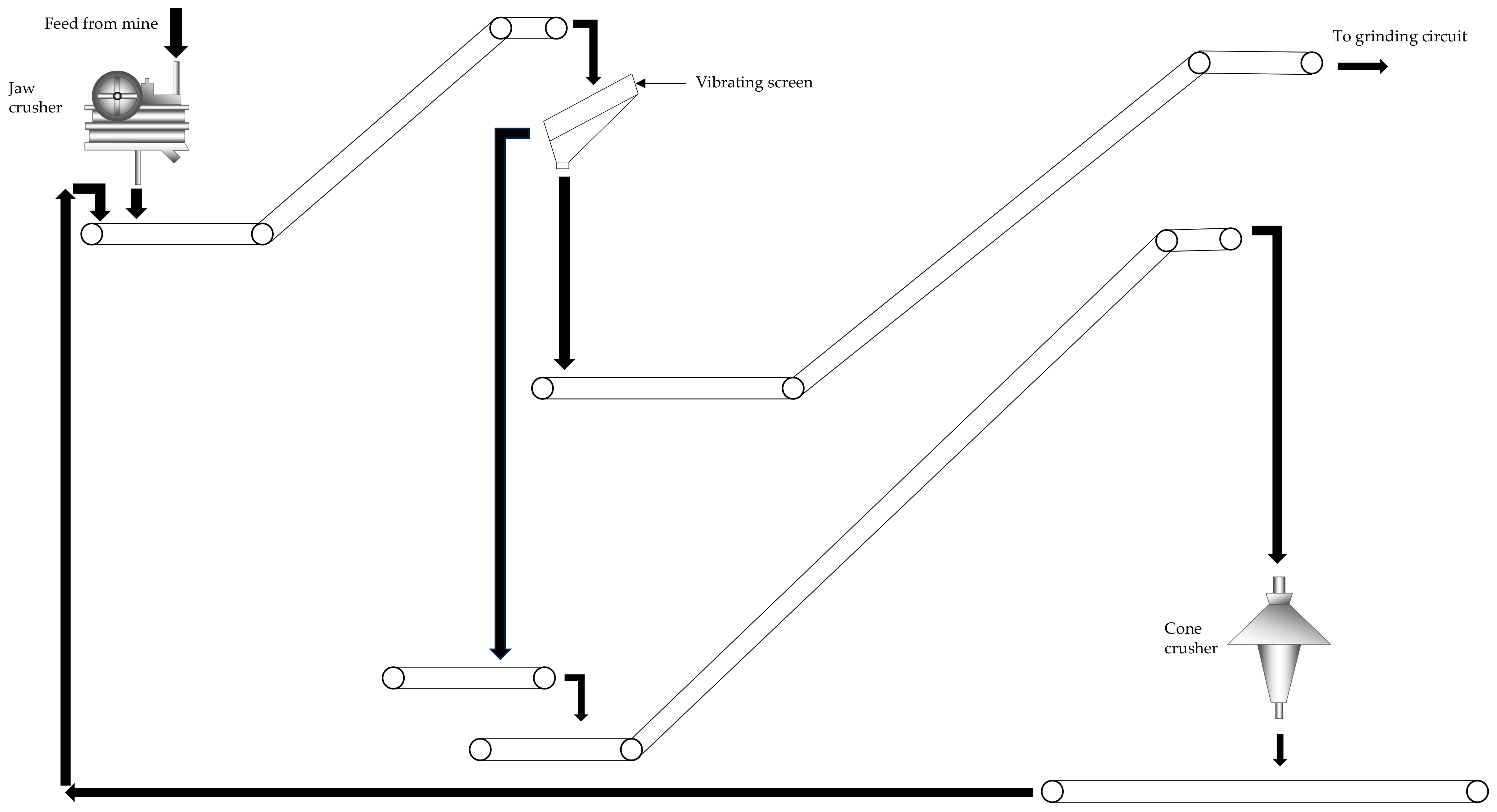
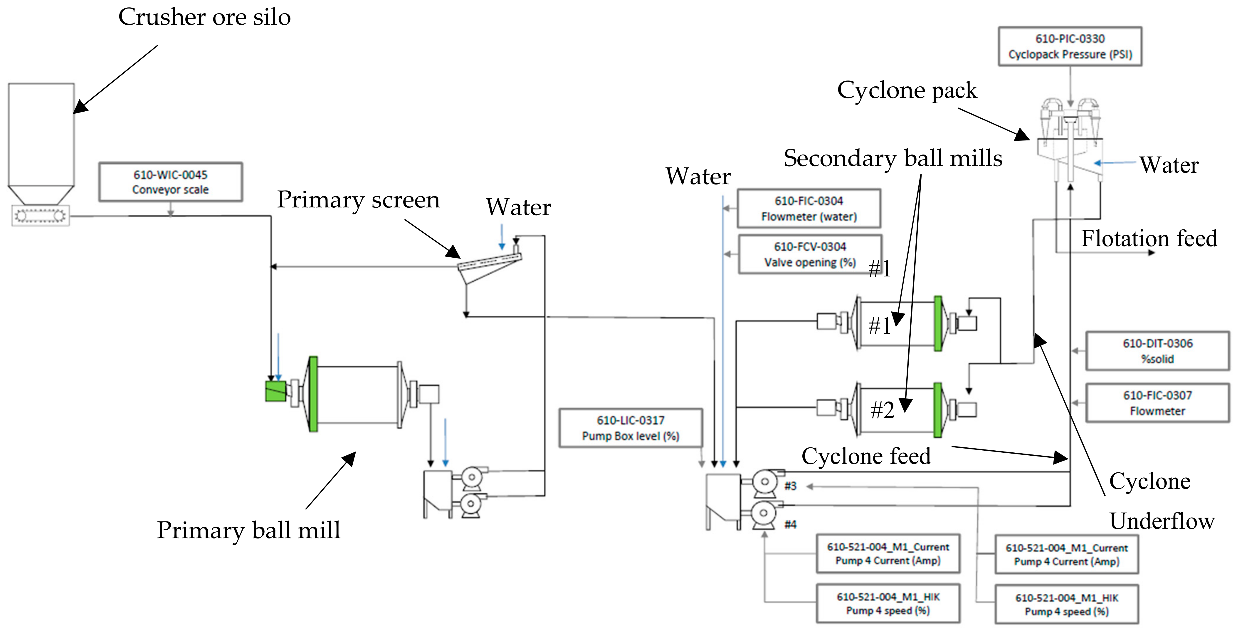
Figure 1 and Figure 2 show the crushing and grinding circuits, respectively. The crushing plant consists of a jaw crusher, which feeds a vibratory screen and two cone crushers (one cone crusher is used as a backup—one cone crusher is shown in Figure 1 for simplicity). The vibratory screen undersize goes to the grinding circuit and the oversize goes to the cone crusher. The cone crusher product is conveyed back to the vibratory screen for classification. The grinding circuit consists of an ore silo, a primary ball mill, a primary vibrating screen, two secondary ball mills in parallel and a cyclone pack. The silo feeds the primary ball mill, and the discharge product goes to the primary screen. The primary screen oversize is recirculated back to the primary ball mill feed. The primary screen undersize is combined with the secondary mills’ discharges in a tank which feeds the cyclone pack. The cyclones’ underflow feeds the secondary ball mills (these mills are in parallel—below 180 t/h, only one secondary ball mill is operated), and the overflow of the cyclone pack is the flotation feed.

Figure 1.
Crushing plant (simplified) at Canadian Royalties’ concentrator.
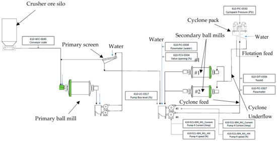
Figure 2.
Grinding circuit at Canadian Royalties’ concentrator.
There were 13 process variables considered; these are summarized in Table 1. The data for these variables were obtained from PI (process information) at the concentrator (the %Pn and %Cp were computed from the nickel and copper data obtained from PI at Canadian Royalties. The NSG was obtained by subtracting the sum of %Pn, %Cp and %Po from 100). The Bond ball work index, mineralogy and primary mill feed (P80) were not used in the PCA because these were not measured daily in a continuous mode.

Table 1.
Nomenclature of parameters used in PCA.
3. Results
The data were cleaned (observations with missing values and observations with a tonnage less than 180 t/h to the primary ball mill were removed). A summary of the cleaned data is shown in Table 2. The data consisted of 189 observations.
Table 2.
Summary of cleaned data.
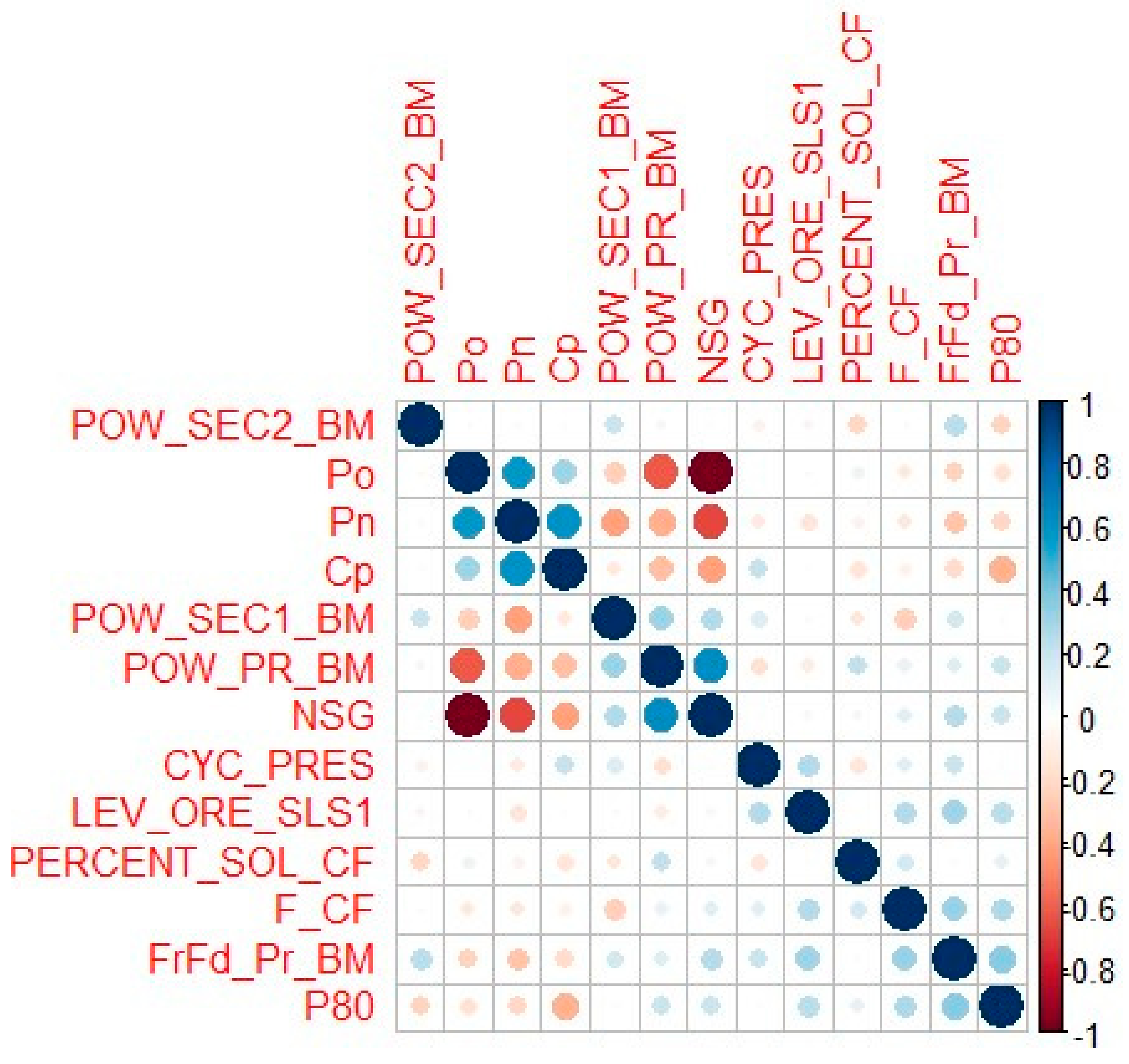
Figure 3 shows the correlation plot for the parameters. The scale is between −1 to +1. A score of −1 means 100% negatively correlated, and +1 means 100% positively correlated. The positively correlated variables are in blue, and the negatively correlated variables are in orange. The bigger and darker the circles, the stronger the correlations and vice versa. This information provides the plant metallurgists with the strength of the correlation between parameters and whether they are positively or negatively correlated. The R (Studio) programming language also provided correlation values (part of the results shown in this paper), and correlations approximately ≤−0.60 and ≥0.60 were considered to be strong. Table 3 illustrates the strong correlations.

Figure 3.
Correlation plot for parameters used in PCA. (The scale on the right is from −1 to 1 in increments of 0.2).
Table 3.
Process parameters with strong correlations.
The correlations between Po versus NSG and Pn versus NSG were negative. This was due to the mineralogy of the ore. As the Po and Pn grades in the feed increased, the NSG decreased and vice versa. The correlation between Pn and Cp was positive; thus, as the grade of Pn increased, the Cp grade increased and vice versa. This was due to the mineralogy of the ore in the feed.
Figure 4 shows the percentage of variance explained versus the principal components. The first principal component explained 28.2% of the variance in the data. The second principal component explained 14.3% of the variance in the data, and as expected, the percentage of variance decreased as a function of the number of principal components. The data’s cumulative variance of 93.36% was explained with nine components.
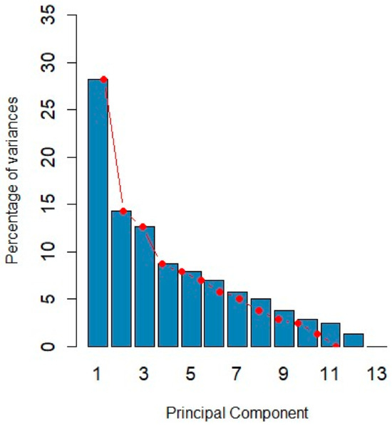
Figure 4.
Percentage of variance explained versus number of principal components.
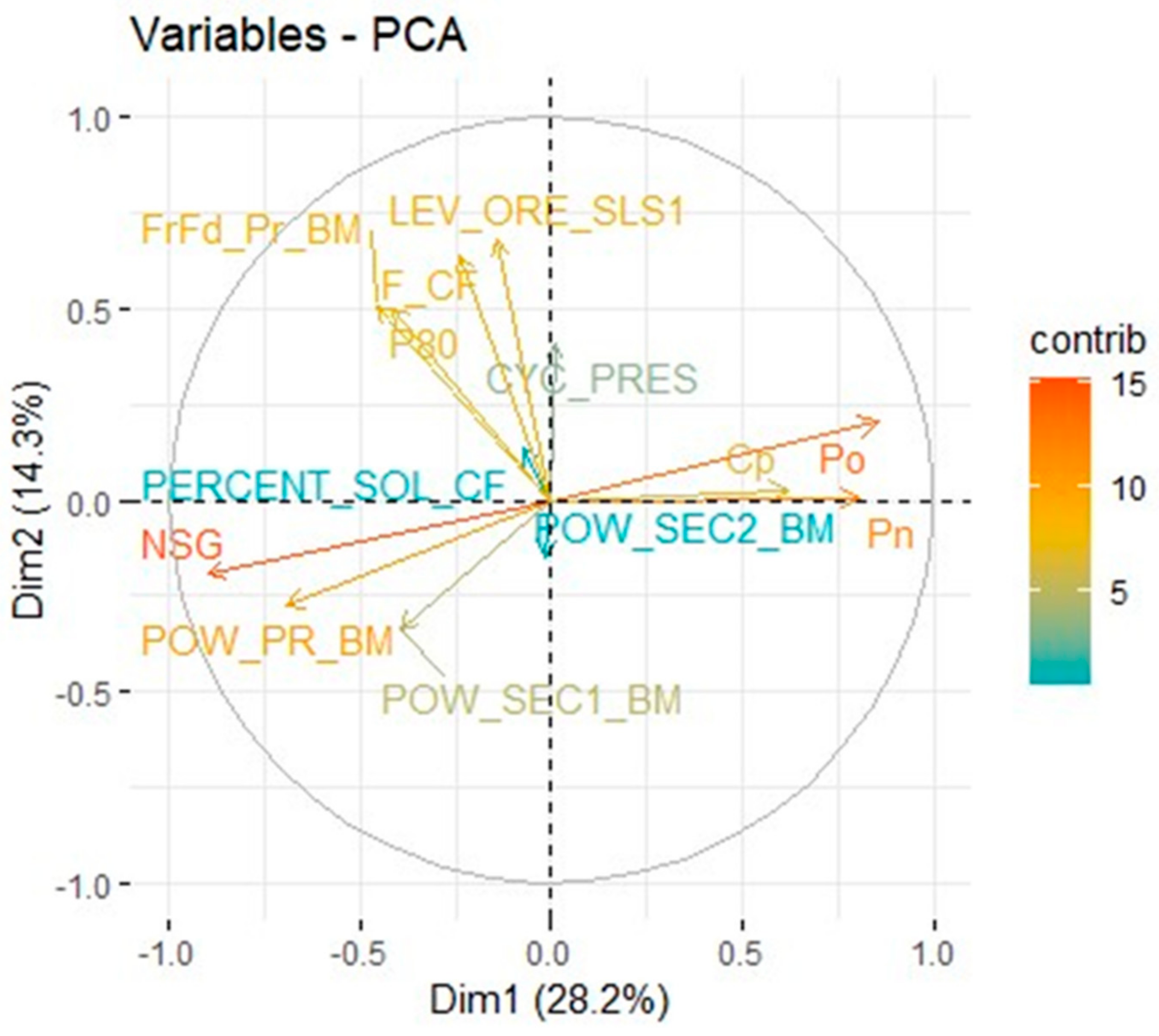
Figure 5 illustrates the graph for Principal Component 2 versus Principal Component 1 for the process variables described in Table 1. The first two principal components accounted for 42.5% of the variance in the dataset. In this graph, if the vectors were perpendicular, there was no correlation between the variables. If the vectors were in the same direction, then the variables increased with one another (positively correlated). If the vectors were in the opposite direction, the variables were negatively correlated (when one increased, the other decreased).
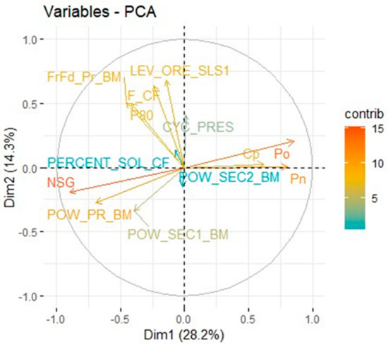
Figure 5.
Principal Component 2 versus Principal Component 2. (Top left quadrant: LEV_ORE_SLS1, FrFd_Pr_BM, F_CF, P80 and PERCENT_SOL_CF. Top right quandrant: CYC_PRES, Cp, Po and Pn., and Bottom left quadrant: POW_PR_BM, NSG, POW_SEC2_BM and POW_SEC1_BM).
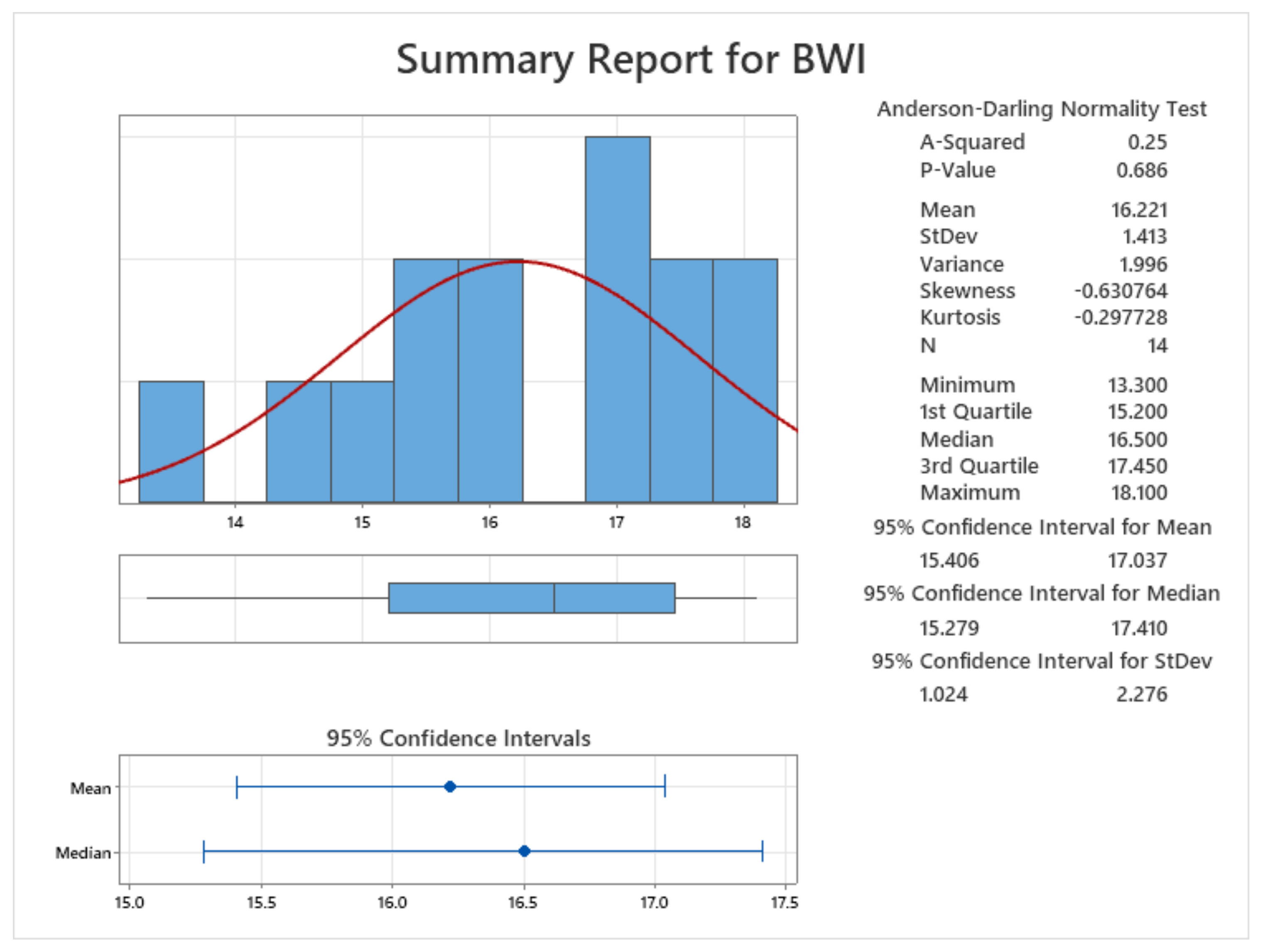
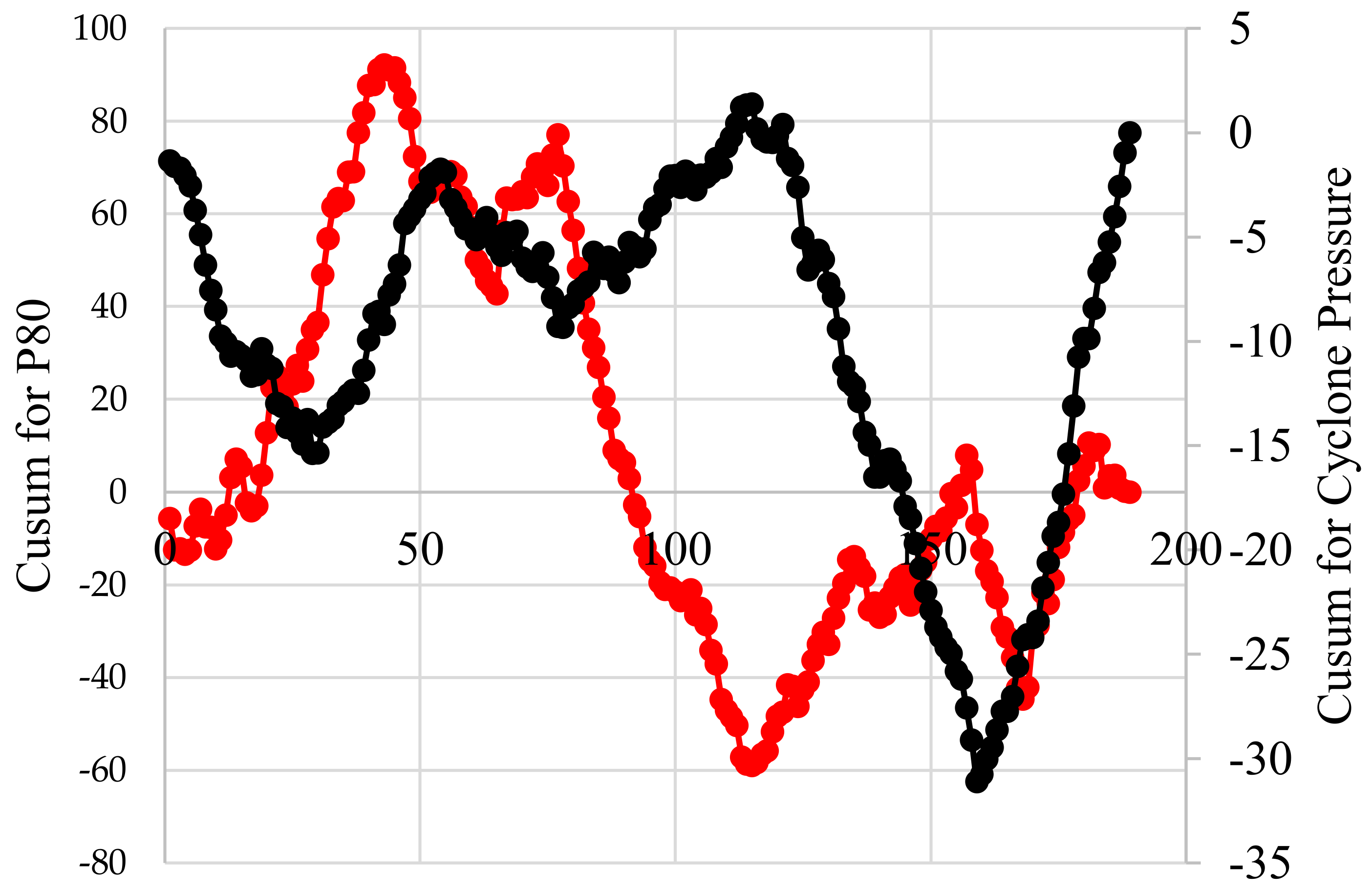
We analyzed the PCA results to determine which factors influenced P80. The Pn, Po, and Cp head grades were almost perpendicular to P80, which implied that they were weakly correlated with P80. P80 and these head grades pointed in the opposite direction to one another, so they were negatively and weakly correlated. Thus, when the Pn, Po and Cp head grades increased, P80 decreased and vice versa. The NSG was almost perpendicular to P80 and pointed in the same direction. Thus, these were weakly correlated. When the NSG increased, P80 also increased but this change was weak due to the high angle between NSG and P80. Nevertheless, the trend was to be expected because the NSG tends to be harder than the sulphides resulting in a coarser P80. Figure 6 illustrates the Bond ball work index (BWI) from September 2019 to May 2020. Most of the BWI scores lay between ~15 kWh/t to ~18 kWh/t, so there were no major changes in feed ore hardness which most likely explains the resulting high angle between NSG and P80, and thus the weak correlation. To further investigate the relationship, a CUSUM chart was plotted for P80 and NSG (Figure 7). For the most part, the CUSUM curves followed each other, which means that when the P80 increased the NSG increased. However, in certain periods the opposite was observed. This is an indication that factors other than NSG impact P80.

Figure 6.
Summary of BWI for September 2019 to May 2020.
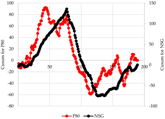
Figure 7.
CUSUM chart for P80 and NSG.
The primary ball mill power, first secondary ball mill power and second ball mill power pointed in the same direction as NSG, but in the opposite direction to Pn, Cp and Po. Also, the angles between the primary ball mill power, first secondary ball mill power and second ball mill power and NSG were low (except for power to the second secondary ball mill) which means that they are strongly correlated. The NSG tends to be harder than Pn, Cp and Po, so we expected to observe the primary ball mill power, first secondary ball mill power and second ball mill power increase as NSG increased. The higher power increase in the mills may be the result of a higher recirculating load (cyclone underflow) due to the ore hardness increasing (higher NSG grade). Despite these observations, P80 was nearly perpendicular to or had a large angle with NSG, Pn, Cp, Po, primary ball mill power, first secondary ball mill power and second ball mill power which meant that the correlation was weak. This implied that other factors such as the throughput to the primary ball mill, silo height, slurry flowrate to the cyclone feed, cyclone feed pressure and percent solids in the cyclone feed had more profound effects on P80; these pointed in the same direction as P80 with a low angle between them.
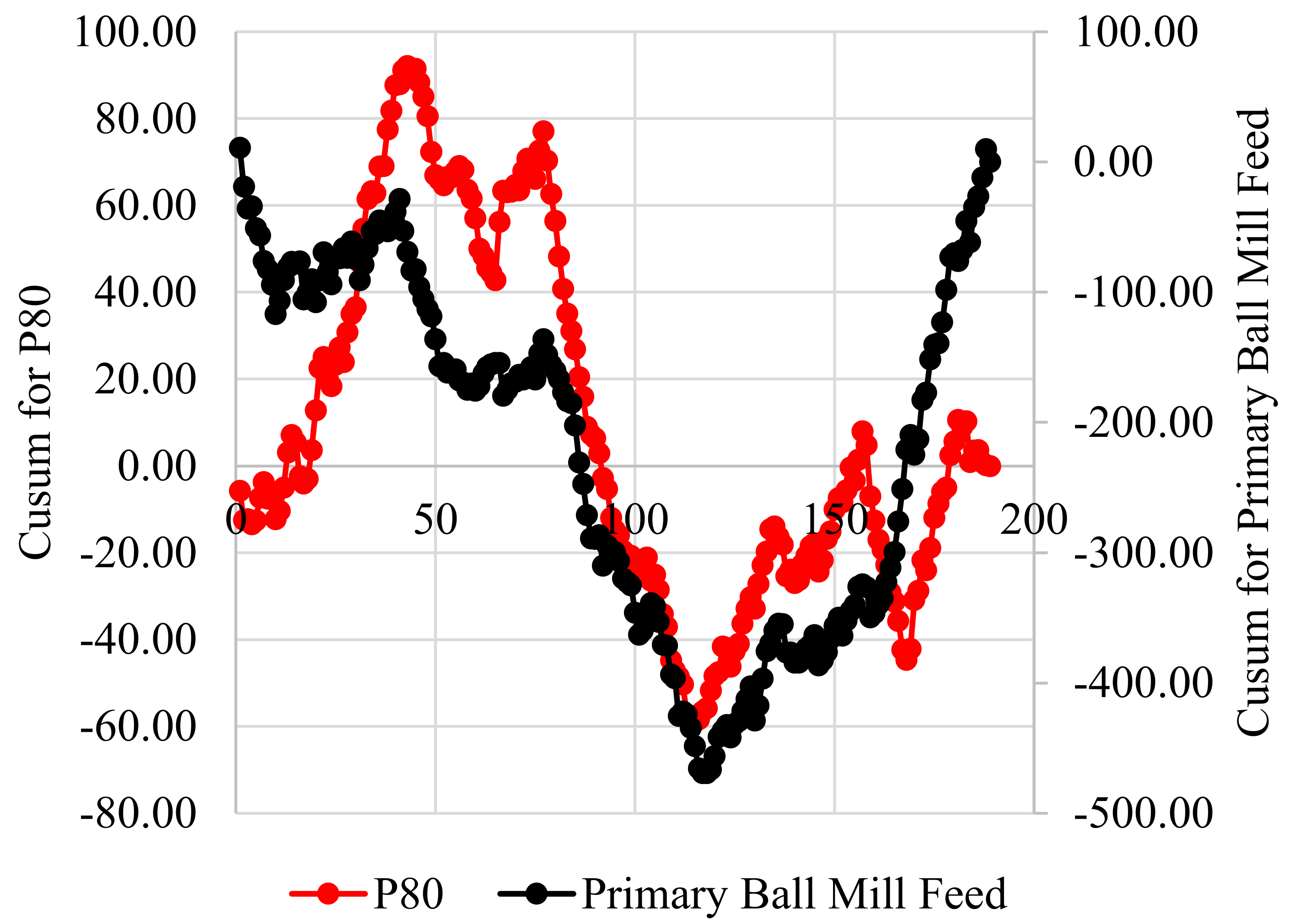
Figure 8 shows the CUSUM chart for NSG and primary ball mill power. Mostly the trends are in the same direction except starting at Observation 125 where they were in the opposite directions. This most likely occurred due to factors other than NSG affecting the primary ball mill power.
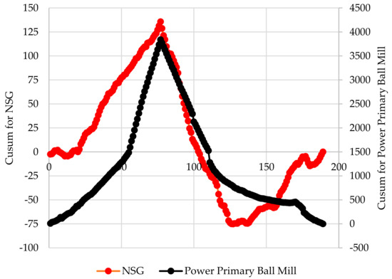
Figure 8.
CUSUM chart for NSG and power primary ball mill.
The angle of the principal components between the power used by the primary ball mill (POW_PR_BM) and P80 was high but slightly less than 90 degrees. This indicated that the power used by the primary ball mill was weakly correlated with P80. Referring to Table 2, the power consumed by the primary ball mill in the first, median and third quartiles were 1431 kW, 1455 kW and 1490 kW, respectively. Thus, the power variation was not high, which most likely resulted in a high principal component angle, meaning that the power was weakly correlated with P80. However, it is important to note that theoretically power can significantly impact P80. This can be observed through the Bond equation shown in Equation (3) [11], where W is the energy input in kilowatts hours per metric ton, Wi is Bond’s work index, P80 is the 80% product size in micrometers and F80 is the 80% feed size in micrometers. From Equation (3), when the energy input is increased (W), the P80 will decrease and vice versa.
Equations (4) and (5) show the cut-size (d50c) and flow rate of the feed slurry to the cyclones (m3/h), respectively [11]. Dc, Di, Do and Du are the cyclone inside diameter, inlet, vortex finder and apex diameters of the hydrocyclone in centimetres, respectively. These parameters did not change. Q represents the volumetric flowrate to a single cyclone (m3/h); this variable is equivalent to F_CF (in our study, F_CF was the slurry flowrate to the cyclone pack). V is the volumetric percentage of solids in feed, h is the distance from bottom of the vortex finder to top of underflow orifice (cm), S is the density of the solids (g/cm3) and L is the density (g/cm3) of the liquid [11]. From Figure 5, when the pressure to the cyclones (CYC_PRES) increased, Q or F_CF increased as well, so this was in accordance with Equation (5) since the higher pulp flowrate in the grind circuit would require higher pressure to feed the cyclones. However, the increase in Q or F_CF should have decreased the d50c according to Equation (4) (when P80 increases the d50(c) increases and vice versa—these are directly proportional); this did not occur, rather the P80 increased. From Figure 5, the P80 (equivalent to d50c) increased when the percent solids to the cyclones (PERCENT_SOL_CF) increased. As throughput increased, if no water was added to the cyclone feed, the percent solids would have increased, causing the P80 to increase. This observation is in accordance with Equation (5) where V increases if the %solids in the cyclone feed (PERCENT_SOL_CF) increase, causing d50c (equivalent to P80) to increase. This is an important point that the plant metallurgist must be aware of. In some cases, production is very important, and the pulp flowrate capacity of the circuit may be reached; thus, the operator may reduce water to allow additional solids in the pulp for higher production. If this occurs, the flowrate to the cyclones (Q or F_CF) also increases with the primary ball mill throughput, and according to Equation (5) the P80 is supposed to decrease but does not due to the higher percent solids in the cyclones feed. These observations indicate that the percent solids to the cyclones had more of an impact on the P80 than the cyclone feed pressure (CYC_PRES), resulting in a higher P80.
Figure 9 illustrates the CUSUM chart for P80 and cyclone pressure. The trend between the CUSUM curves should be in the opposite direction according to Equations (2) and (5). However, it was not always the case; in certain instances, they were in the same direction, which means factors other than the cyclone pressure affected P80. Figure 10 shows the CUSUM chart for P80 and percent solids. The CUSUM curves moved in the same direction, which means that when percent solids increased, P80 increased and vice versa; this is in accordance with Equation (4). However, during certain periods the opposite was observed. This means that other variables affected P80.

Figure 9.
CUSUM chart for P80 and cyclone pressure.
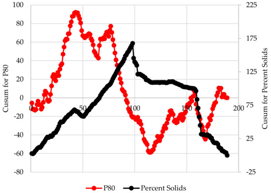
Figure 10.
CUSUM chart for P80 and percent solids.
When the silo level (LEV_ORE_SLS1) increased, the cyclone feed pressure (CYC_PRES), percent solids to the cyclone feed (PERCENT_SOL_CF), P80, pulp flowrate to the cyclone feed (F_CF) and ore feed rate to the primary ball mill (FrFd_Pr_BM) increased, since all the arrows pointed in the same direction and the angles were low. This implied that the variables were positively correlated and significantly affected P80. When the silo height was high, most likely finer particles exited the silo (Perron, 2024) [12] resulting in a higher primary screen underflow. This higher flowrate of the primary screen underflow caused the residence time of the pulp in the secondary ball mill circuit to decrease, the lower residence time in the secondary ball mills meant that less grinding occurred and caused the feed flowrate to the cyclones and percent solids in the cyclone feed to increase, resulting in a higher P80. When the silo level decreased, most likely coarser particles exited increasing the particle size distribution of the primary ball mill feed and possibly these may be harder than the finer particles [12]. This change will cause the recirculating loading in the primary ball mill to increase [12]. Thus, the feed tonnage or throughput will have to be decreased so as not to overload the primary ball mill [12]. Another effect of the higher particle size distribution is the decrease in the primary screen undersize flowrate, pressure of slurry to the cyclone feed, percent solids to the cyclone feed and pulp flowrate to the cyclone feed. The lower flowrate (cyclone underflow) to the secondary ball mill circuit will increase the residence time; the higher residence time in the secondary ball mills meant that more grinding occurred, most likely resulting in a finer grind or P80. The relationship between the primary ball mill throughput and P80 is shown in the CUSUM plots in Figure 11. The two CUSUM curves mainly move in the same direction, showing that when throughput to the primary ball mill increased, the P80 increased and vice versa. Houhamdi et al., 2022 [13], performed DEM simulations to determine the normal and tangential pressures of dry wheat in silos. They found that in silos the normal and tangential pressures vary as a function of height. The tangential pressure is the highest at the cylindrical and hopper transition [13]. Thus, it may be that at high silo heights, the high tangential pressure may delay the exiting of coarser particles and facilitate the existing of the finer particles; then when the silo height decreased the coarse particles’ exit due to the lower tangential pressure is the highest at the cylindrical and hopper transition. The author (Antonio Di Feo) of this manuscript made a similar observation while working as a metallurgist at a nickel concentrator. At low silo heights, the particle size distribution of the SAG feed coarsened, resulting in higher KPAs in the SAG, which lowered the throughput and vice versa.

Figure 11.
CUSUM chart for P80 and primary ball mill feed.
To achieve greater uniformity or reduced variance in P80, control measures must be applied to the feed rate or throughput to the primary ball mill (FrFd_Pr_BM) and silo level (LEV_ORE_SLS1). A strategy to implement these features would need to be developed and implemented in the grinding circuit. However, it is important to note that tonnage is maximized to maximize revenue for Canadian Royalties. In certain cases, the tonnage cannot be maximized; for example, when maintenance is performed in the concentrator, the tonnage is lowered to avoid emptying the silo. Also, there most likely was a segregation phenomenon in the silo when the crushing plant was stopped for maintenance. As time elapsed after the shutdown of the crushing plant, only coarse particles remained in the silo; thus, the tonnage had to be reduced to avoid instability in the flotation circuit. Factors other than the P80 have to be considered in the control of tonnage, which must be investigated after this study.
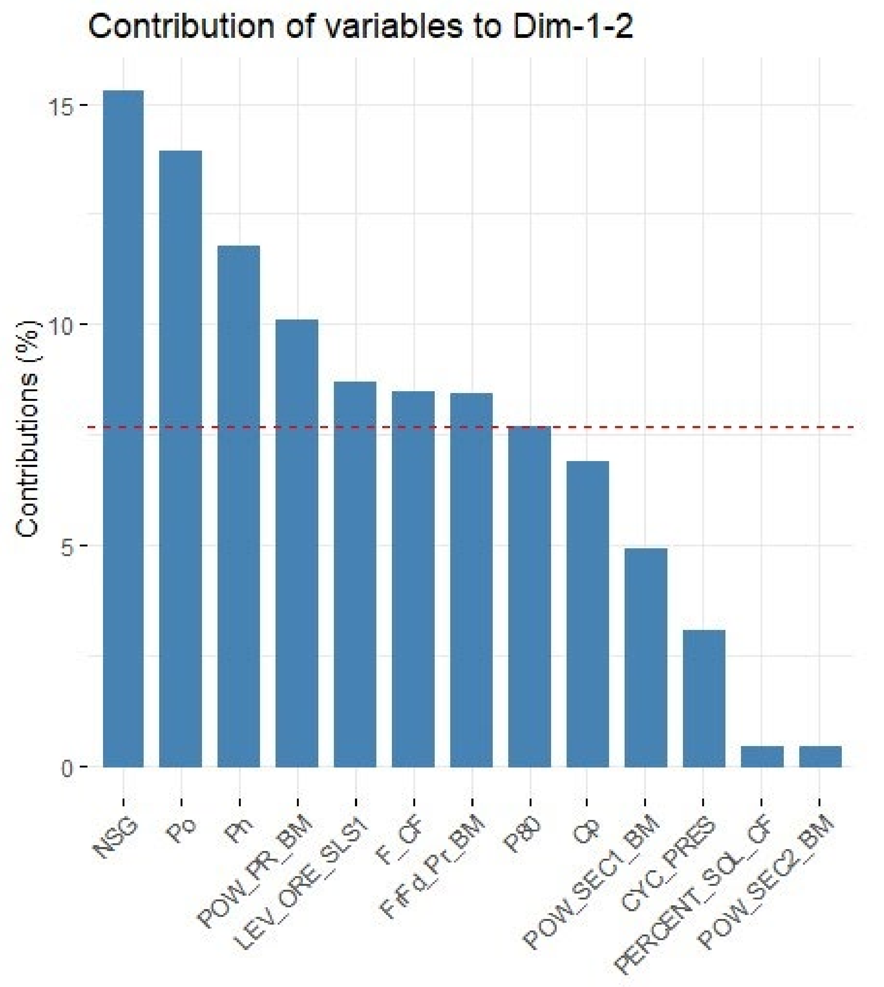
Figure 12 illustrates the percent contributions of the process parameters for thirteen variables to Principal Components 1 and 2. The percentage of the parameter contribution decreases from left to right. For example, NSG head grade contributed the highest to the Principal Components 1 and 2, followed by Po head grade, etc. Secondary ball mill #2 power made the lowest contribution to the Principal Components 1 and 2. The results presented in Figure 12 are equivalent to the “contrib” (contribution) bar in Figure 5. For example, NSG has the highest contribution to Principal Components 1 and 2 in Figure 12 and has a dark orange colored arrow in Figure 5, indicating a high contribution to Principal Components 1 and 2.

Figure 12.
Percent contribution of parameters for the sixteen principal components to Dim 1 (Principal Component 1) and Dim 2 (Principal Component 2). Red dotted line represents half of the contribution on the y-axis.
4. Discussion
Researchers have used different methods than PCA for the control of grinding circuits. The technique used in this manuscript serves to guide the plant metallurgists in what changes to make to control the P80 in the plant. It does not serve as a predictive tool for P80. The limitation of PCA (unsupervised technique) is that the P80 cannot be predicted and it can only be used as a guideline.
There are machine-learning methods other than PCA that can be used to control grinding parameters, and each one is different. Each method has its advantages and disadvantages, for example, level of difficulty and ease of application, etc. Al Bannoud et al., 2022 [4], used artificial neural network model predictive control (NNMPC) for dry grinding in a closed circuit with a ball mill. They developed models to predict the quantity of finer particles produced. Mitra and Ghivari, 2005 [6], used feed-forward neural networks (FNN) and wavelet-frames for the modelling of wet grinding lead–zinc operation. They generated input–output data by running numerous simulations from a phenomenological and empirical model of the same industrial operation. They used the solid stream of ore and water streams to the primary and secondary sumps as input variables. The output variables used were throughput, percentage of +150 μm, −63 μm and −38 μm, recirculation load and %solids in the final output stream. They found that the technique to be suitable in fitting the data. Koh et al., 2022 [7], developed the automated machine-learning (AutoML) technique for automated machine-learning models with almost no user machine-learning knowledge. They tested this concept in three operations. These models were used to model preconcentration, blasting and comminution conditions for miner scheduling. Also, a flotation model was used to identify the best comminution circuit operating conditions to maximize metal production. Olivier et al., 2022 [8], used GoogLeNet in transfer learning mode to classify the particle size distribution of the underflow of a pilot-scale hydrocyclone using images of the underflow. PCA is different from the technique mentioned above; it reveals the trends in the data or how the parameters are related, which can be used as a guideline in controlling the grinding circuit.
The present findings can be used by the plant metallurgists at Canadian Royalties to reduce variation in the P80 of the cyclone overflow (feed to flotation). The values in Table 2 can be used as a guideline. For example, if the silo height decreases below ~56% then the P80 will decrease to <60 μm. In this case, the metallurgists should not add grinding media to the ball mills to avoid overgrinding, for example. If the silo height increases above ~82%, then the P80 will increase to greater than ~66 μm and if the height increases further to ~92%, then the P80 can be as high as ~77 μm. In this event, the metallurgists should avoid overfilling the silo, and if the height of the silo is too high, then more grinding media should be added to the primary ball mill and/or the secondary ball mills, if possible, for example. As another example, if the throughput to the primary ball mill is increased, then according to Figure 5 the %solids to the cyclone feed will also increase, resulting in a higher P80. In this case, more water should be added to the cyclone feed to avoid the P80 increasing. These are just a few examples as to how the information obtained can be used in the plant. Of course, the changes will have to be performed according to the mineral processing principles or theory.
The daily mineralogy and hardness of the ore were not available, but the calculated Pn, Cp, Po (calculated by Canadian Royalties and included in the data sent to CanmetMINING) and NSG head assays were included in the PCA analysis to infer changes in feed mineralogy and hardness. These two parameters are extremely important; however, the concentrators cannot measure these on a daily basis due to budget and resource availability. Therefore, the calculated head assays were included in the PCA analysis to indirectly infer changes in the feed hardness and mineralogy. Changes in these two parameters will impact the circulating load in the crushing and grinding circuits, causing fluctuations in the P80. The monthly composite hardness test results (Bond work index—BWI) and head assays from September 2019 to May 2020 were available. The BWI did not vary significantly (~15 kWh/t to ~18 kWh/t). This meant that most likely the ore hardness and mineralogy of the feed did not change significantly, which may explain the weak correlation between these variables and P80 (high angles between these variables and P80 in Figure 5). Having this information will allow the plant metallurgist to adopt strategies in the grinding circuit to avoid the impact of the head grade on P80. For example, if the NSG increases then the P80 will increase, then in this case the tonnage may be reduced to avoid the P80 becoming too coarse (although this is unlikely to happen because the revenue would be lowered). Again, the principles or theory of mineral processing will have to be followed.
The PCA technique can be applied by metallurgists to grinding circuits at other concentrators. Future research can focus on the linking of a PCA model to another model that can predict P80, in other words, to have an unsupervised coupled model with a supervised model. If research on such an approach is conducted, then the plant metallurgists can not only determine the trend in the P80, but they can know when to take corrective actions based on the supervised model (a model that predicts P80). Also, Canadian Royalties should pursue the PCA study with data from longer periods of time, for example, more than 1 year of data, to take into account ore variability characteristics and seasonal variations which will improve the robustness of the PCA analysis.
Another factor that will have to be considered is equipment maintenance. If the equipment is not maintained at regular intervals, for example, grinding mills, then the equipment will not perform in the manner that was designed. Thus, when the equipment is repaired, it will not perform at the same capacity and may induce inaccuracies in the PCA or other artificial intelligence models.
The Canadian Royalties concentrator is recommended to measure the circulating load in the secondary ball mill circuit and control the percent solids to the cyclone feed (add water to the cyclone feed when the throughput increases). Ideally, the circulating load is recommended to be between 250 and 300% to avoid overgrinding. It would be interesting to include this parameter in the PCA and determine how it relates to the other factors, especially P80. An online particle size analyzer is also recommended to monitor the P80 continuously. This would allow the plant metallurgists to better control the crushing and grinding circuit to achieve the desired P80.
PCA in this work provides the metallurgists with an overview or holistic approach to the data in the grinding circuit at Canadian Royalties, more specifically, trends in the data. However, the metallurgist is recommended to use fundamental principles to make corrective actions in the grinding circuit.
5. Conclusions
PCA is a valuable technique to analyze large datasets. It reduces the number of components required to explain trends in the data. We applied this statistical technique to uncover data trends affecting the grinding circuit’s P80 at Canadian Royalties Inc’s concentrator.
- (1)
- The P80 was directly correlated with the following variables; thus, when these variables increased, the P80 increased.
- (a)
- Feed tonnage to the primary ball mill (FrFd_Pr_BM);
- (b)
- Silo level (LEV_ORE_SLS);
- (c)
- Pulp flowrate to the cyclone feed (pack) F_CF;
- (d)
- Pressure CYC_PRES;
- (e)
- Percent solids to cyclone pack (PERCENT_SOL_CF).
- (2)
- The head grades (Pn, Cp and Po) and P80 exhibited near-perpendicular relationships and pointed in opposite directions, indicating a weak negative correlation.
- (3)
- The NSG head grade and P80 exhibited near-perpendicular relationship and pointed in the same direction, indicating a weak positive correlation.
- (4)
- The study illustrates how large datasets can be used to understand trends in the data for the grinding circuit. The same techniques can be used in other areas, for example, flotation circuits, thickening circuits, gravity separation, etc. It facilitates the metallurgists’ tasks to retrieve meaningful trends to make informed decisions in their operations.
Author Contributions
A.D.F. performed the R programming and the artificial intelligence analysis and wrote the article. N.K. cleaned the data received from Canadian Royalties and prepared it for analysis (R programming and statistical analysis). He reviewed the article. M.G. and S.M. provided the data to CanmetMINING and reviewed the article. All authors have read and agreed to the published version of the manuscript.
Funding
This research received no external funding.
Data Availability Statement
Data is confidential to Canadian Royalties.
Acknowledgments
The authors would like to thank CanmetMINING and Canadian Royalties Inc. for permission to publish this article. Tesfaye Negeri, Shahrokh Shahsavari, Maziar Sauber, Eliza Ngai, Kristie Tarr, Bryan Tisch and Magdi Habib for reviewing the article.
Conflicts of Interest
Antonio Di Feo and Nasseh Khodaie are employed by Natural Resources Canada. The remaining authors declare that the research was conducted in the absence of any commercial or financial relationships that could be construed as a potential conflict of interest.
References
- Ge, Z.; Song, Z.; Ding, S.X.; Huang, B. Data Mining and Analytics in the Process Industry: The Role of Machine Learning. IEEE Access 2017, 5, 20590–20616, Special section on data–driven monitoring, fault diagnosis and control of cyber-physical systems. [Google Scholar] [CrossRef]
- Beck, D.A.; Carothers, J.M.; Subramanian, V.R.; Pfaendtner, J. Data Science: Accelerating Innovation and Discovery in Chemical Engineering. AIChE J. 2016, 62, 1402–1416. [Google Scholar] [CrossRef]
- McCoy, J.T.; Auret, L. Machine learning applications in minerals processing: A review. Miner. Eng. 2019, 132, 95–109. [Google Scholar] [CrossRef]
- Al Bannoud, M.; Dias Martins, T.; Ferreira dos Santos, B. Control of a closed dry grinding circuit with ball mills using predictive control based on neural networks. Digit. Chem. Eng. 2022, 5, 100064. [Google Scholar] [CrossRef]
- Tohry, A.; Yazdani, S.; Hadavandi, E.; Mahmudzadeh, E.; Chehreh Chelgani, S. Advanced modelling of HPGR power consumption based on operational parameters by BNN: A “Conscious-Lab” development. Powder Technol. 2021, 381, 280–284. [Google Scholar] [CrossRef]
- Mitra, K.; Ghivani, M. Modeling of wet grinding using artificial intelligence-based techniques. In Proceedings of the 16th Triennial World Congress, Prague, Czech Republic, 3–8 July 2005. [Google Scholar]
- Koh, E.J.Y.; Amini, E.; Gaur, S.; Becerra Maquieira, M.; Jara Heck, C.; McLachlan, G.J.; Beaton, N. An Automated Machine Learning (AutoML) approach to regression models in minerals processing with case studies of developing industrial comminution and flotation models. Miner. Eng. 2022, 189, 107886. [Google Scholar] [CrossRef]
- Olivier, J.; Aldrich, C.; Liu, X. Explaining Convolutional Neural Network Predictions of Particle Size in the Underflow of a Hydrocyclone. IFAC Pap. 2022, 55, 19–24. [Google Scholar] [CrossRef]
- James, G.; Witten, D.; Hastie, T.; Tibshirani, R. An Introduction to Statistical Learning; Springer: Berlin/Heidelberg, Germany, 2017. [Google Scholar]
- Johnson, R.A.; Wichern, D.W. Applied Multivariate Statistical Analysis; Pearson Modern Classic: Upper Saddle River, NJ, USA, 2019. [Google Scholar]
- Wills, B.A. Wills’ Mineral Processing Technology, An Introduction to the Practical Aspects of Ore Treatment and Mineral Recovery, 8th ed.; Elsevier: Amsterdam, The Netherlands, 2016. [Google Scholar]
- Perron, J.; (Chief Metallurgist at Canadian Royalties, Montreal, QC, Canada). Personal communication, 2024.
- Houhamdi, B.; Djeghaba, K.; Gallego, E. Particle Size Effect on DEM Simulation of Pressures Applied on a Cylindrical Silo with Hopper. Period. Polytech. Civ. Eng. 2022, 66, 653–669. [Google Scholar] [CrossRef]


Disclaimer/Publisher’s Note: The statements, opinions and data contained in all publications are solely those of the individual author(s) and contributor(s) and not of MDPI and/or the editor(s). MDPI and/or the editor(s) disclaim responsibility for any injury to people or property resulting from any ideas, methods, instructions or products referred to in the content. |
© 2024 by the authors. Licensee MDPI, Basel, Switzerland. This article is an open access article distributed under the terms and conditions of the Creative Commons Attribution (CC BY) license (https://creativecommons.org/licenses/by/4.0/).