


Evolution of Pore Spaces in Marine Organic-Rich Shale: Insights from Multi-Scale Analysis of a Permian–Pennsylvanian Sample
1
School of Energy Resources, China University of Geosciences (Beijing), Beijing 100083, China
2
Key Laboratory of Marine Reservoir Evolution and Hydrocarbon Enrichment Mechanism, Ministry of Education, Beijing 100083, China
3
Oil and Gas Survey, China Geological Survey, Beijing 100083, China
*
Authors to whom correspondence should be addressed.
Minerals 2024, 14(4), 392; https://doi.org/10.3390/min14040392
Submission received: 8 March 2024
/
Revised: 30 March 2024
/
Accepted: 7 April 2024
/
Published: 10 April 2024
(This article belongs to the Topic Reservoir Characteristics and Evolution Mechanisms of the Shale)
Abstract
:The quantitative evolution pattern of pore space and genetic pore types along the maturation process in organic-rich shale reservoirs is unclear, which affects the assessment of shale storage capacity and petroleum production. A black shale outcrop sample from Kansas that is of Permian–Pennsylvanian age was collected and subjected to thermal simulation experiments at 10 different maturity stages to understand the pore sizes and pore types. Scanning electron microscopy (SEM) and image processing were used to characterize the full-scale pore-size distribution and volume evolution of this shale sample by combining low-temperature gas (CO2 and N2) physisorption and mercury intrusion porosimetry (MIP) in order to discuss the effects of hydrocarbon generation and diagenesis (HG&D) on pore development at different pore sizes. The study showed that the original shale sample is dominated by slit-like pores, with mainly organic matter (OM) pores distributed in 0–100 nm, intraparticle pores (Intra-P) of clays distributed in 30–100 nm, and interparticle pores (Inter-P) distributed in 100–1000 nm. With the increase in maturity or Ro, the OM pores increased gradually, and the OM pore-size distribution diverged to the two poles. In the oil generation stage, the OM pores were distributed in the range of 30–100 nm, while in the gas generation stage, the OM-hosted pores were mainly distributed in the range of 10–20 nm and 100–500 nm. Further into the over-maturity stage, the OM pores were mainly distributed in the range of 0–10 nm and >100 nm. The pore volume distribution across the whole pore sizes showed that the pore volume of low-maturity shale samples was mainly provided by 100–1000 nm (macropores), and the pore volumes of 0–2 nm, 30–100 nm and 1000+ nm pores gradually increase with increasing thermal maturity, with the final pore-size distribution having four peaks at 0–2, 30–100, 500–1000 nm, and 10–100 µm. Hydrocarbon generation mainly affects the pore volume in the 0–2 nm and 100–1000 nm intervals, with a positive correlation. The 2–30 nm and 30–100 nm pores were likely controlled by diagenesis, such as mineral transformation, illitization, and cementation during the maturation process.
1. Introduction
Shale oil and gas are unconventional resources generated and stored in the interlayers of organic-rich mud or shale, mainly present in the adsorbed and free states [1,2,3,4]. With the increasing success of shale oil and gas development in North America and China [5,6], it has become an important component of future fossil fuels. For shale petroleum systems, shales themselves are source rocks that produce hydrocarbons during the process of continuous deep burial [7]. However, shales are reservoirs as well, where pores generated by the diagenesis of minerals and thermal evolution of organic matter provide sites for hydrocarbon storage [8,9]. Due to the features of source-reservoir integration, the joint effects of hydrocarbon generation and diagenesis (HG&D) on pore evolution have become the hotspot for geological studies of shale oil and gas [10,11].
According to the classification of the International Union of Pure and Applied Chemistry (IUPAC), pore sizes are classified into micropores (<2 nm), mesopores (2–50 nm), and macropores (>50 nm) by diameter [12], but there is a mismatch between the classification and pore types developed during shale maturation, and it is difficult to elaborate the intrinsic connection between HG&D and pore evolution. Loucks, Reed, Ruppel and Jarvie [13] first classified the genesis type of shale pores using Ar-ion milling and SEM imaging. With the development of computing resources and image recognition techniques (IRT), it has been possible to quantify pores in images from ~1 nm up, but the small observational area and the strong heterogeneity of shale make the quantification of pores by SEM images still limited [14,15,16,17,18]. For the quantitative characterization of the whole pore-size distribution of shales, pores of the three sizes (0–2, 2–50 and >50 nm) are mostly characterized by the combined method of mercury intrusion porosimetry (MIP), low-temperature N2 and CO2 physisorption, and nuclear magnetic resonance [19,20,21,22,23], but the inability to observe the pore morphology and certain assumptions-based processing make the characterization results less meaningful for geological theories and exploration practice.
Thermal simulation experiments carried out at a succession of consecutively high temperatures are regarded as a feasible way to model the longtime low-temperature geological development process in a relatively short experimental period, according to the time-temperature compensation theory put forward by Connan [24]. Originally, thermal simulation experiments were mainly used to reveal the hydrocarbon potential and diagenesis of source rocks [25,26]. With the growing interest in micro- and nano-pores in shales, thermal simulation experiments have been expected to be used to study the evolution of shale oil and gas reservoirs in recent years [10,11]. However, because shale oil and gas reservoirs were always highly mature and ancient rocks that had undergone long-term burial, the organic matter, minerals and fluids within them had already undergone thermal evolution and exchange, making most shales unavailable for thermal simulation experiments. Scholars have used contemporaneous outcrop samples or shallowly buried samples as substitutes [10,11,27,28,29], but many of them have undergone the early oil generation stage, resulting in loss of oil and cessation of early diagenesis.
Combining thermal simulation experiments, SEM and IRT, and whole pore-size characterization methods will help to explore multi-scale pore evolution from pore genesis classification and clarify the effects of HG&D on pore evolution. In this study, immature shale samples (Ro = 0.64%) in Permian–Pennsylvanian were collected on gold tube thermal simulation experiments with water-bearing closure conditions, SEM, MIP and low-temperature gas adsorption (LTGA, using N2 and CO2) were used to characterize the pore structure and whole pore size (0–1000+ nm in dia.) -pore volume distribution of shales at different maturity stages based. The pore evolution was quantified in the intervals of 0–2 nm, 2–30 nm, 30–100 nm, 100–1000 nm, and 1000+ nm, and the effects of HG&D on multi-scale pore evolution were discussed.
2. Geological Setting
Pennsylvanian black shales, pervasive across the central continental United States, have been extensively examined in outcrops as the principal unit of the classic Midcontinent cyclothem (Figure 1). These shales were formerly regarded as exhibiting a high condensation profile within the stratigraphic sequence geological paradigm [30]. In Kansas, they are often thinly bedded but widely distributed as distinctive lithologic outcrops. The organic-rich black shale is consistently present, characterized by its limestone richness, and deposited under open oceanic conditions. Most were formed offshore in deep water under calm, stagnant conditions [31]. Shale samples exhibit elevated levels of total organic carbon (TOC) and low maturity characteristics due to their deposition in deep offshore waters and shallow burial depths (Table 1). Their similar composition to the Barnett and Woodford Shales, primarily comprising calcite, quartz, and clay [32,33,34], renders them suitable for thermal simulation experiments and pore evolution studies of marine shales.
3. Methods
3.1. Thermal Simulation Experiment
Hydrothermolysis in a closed system was used to simulate the formation conditions and to cover the water consumed by OM pyrolysis and water–rock interactions. First, the sample was divided into 11 subsamples of 1 g in weight, each of which was ground to 10–15 mesh. The first sample was the original sample and was tested for TOC and vitrinite reflectance (Ro). The other 10 subsamples were separately sealed into gold tubes under the protection of argon and placed in an autoclave filled with water. To facilitate the kinetic reactions involved in organic matter hydrocarbon generation and mineral transformation [35], a heating rate of 20 °C/min was chosen as the experimental heating rate. The samples were heated to 200, 250, 300, 350, 400, 450, 500, 550, 600, and 650 °C under 20 °C/min heating rate and a 50 MPa confining pressure. After heating, the gold tube was punctured to release the gas into the vacuum system. A GC-6890 gas chromatograph (Purui Instruments, Beijing, China) was used to quantify the gaseous hydrocarbons (C1–C5), and then the liquid light hydrocarbons (C6–C14) were quantified using the internal standard method [28]. The solid residue was filtered, and the organic solvent was evaporated, followed by the weighing of heavy hydrocarbons (C14+). The procedures and details of the thermal simulation experiments can be found in Wang and Guo [28], Yang and Guo [36]. The solid residue was dried at 60 °C and then tested for X-ray diffraction (XRD), low-temperature gas physisorption, MIP, and Ro analyses.
3.2. Vitrinite Reflectance (Ro)
The solid residue adhered to the surface of the plate and was polished. The Ro was measured with a Leica DMRX microscope equipped with a 3Y Post Pro V.2.0.0 microspectrophotometer (Leica Instruments, Wetzlar, Germany). Twenty particles of vitrinite were measured at least in each sample, and the final vitrinite reflectance was obtained according to the average value.
3.3. X-ray Diffraction
The whole-rock minerals were analyzed using a D8 DISCOVER X-ray diffractometer (Brooke Scientific Instruments, Billerica, MA, USA). The shale samples were crushed and ground to particle sizes below 40 μm, made into tablets using the back compression method, and uploaded to the instrument to obtain a diffraction pattern from 3° to 45° at room temperature and 35% humidity [37]. The relative content of minerals was calculated using the area of the main peak corresponding to each mineral and Lorentz polarization correction [38].
3.4. Pore-Size Characterization Methods
The pores of the subsamples after thermal simulation were measured by LTGA (N2 and CO2) and MIP, respectively. The subsamples were screened by a 100 mesh sieve before testing.
An Autopore IV9500 automatic mercury injection meter (Huapu General Technology Co., Ltd., Shenzhen, China) was used for MIP tests. The mercury was slowly pressed into the pores of the evacuated sample as the pressure was slowly increased from a vacuum (~0 MPa) up to 400 MPa and then reduced to atmospheric pressure (0.11 MPa), during which the mercury volume change was recorded. The relationship between capillary pressure and area was calculated based on the Young–Dupre equation and Washburn equation, which was then used to characterize the pore volume distribution by the correspondence between pore diameter and pressure [39,40].
A Quadrasorb SI analyzer (Quantachrome Instruments, Boynton Beach, FL, USA) was used for low-temperature N2 adsorption analyses. The sample was incrementally contacted with N2 at 77.37 K until the mass remained constant at each relative pressure (P/P0) from 0.01 to 1.0. The adsorbed N2 volume is a function of the relative pressure, and the pore volume distribution was calculated by the BJH model [41], which established the relationship between the relative pressure (P/P0) and the pore size.
A NOVA4200e analyzer (Quantachrome Instruments, Boynton Beach, FL, USA) was used for the low-temperature CO2 adsorption tests. The maximum balanced pressure was 0.1 MPa at 273 K. Since the saturation vapor pressure (P0) of CO2 is 3.48 MPa at this temperature and pressure, the relative pressure variation range was 0~0.03. The pore-size distribution was calculated based on density functional theory (DFT) [7].
3.5. SEM and IRT
FEI Quanta 200F FESEM (FEI company, Hillsboro, OR, USA) was used to observe the subsamples after thermal simulation. The samples were polished with 3000 grit sandpaper, milled with argon ion and sprayed with gold before observations. The SEM images were filtered to remove noise, and the pores were binarized using grayscale thresholding. The number, area and proportion of pores were counted by ImageJ software (version 1.8.0) [42,43,44].
4. Results
4.1. Maturity and Hydrocarbon Yield
Ro is the classic indicator of maturity, and our discussion on pore development will revolve around different Ro values from 10 thermally matured samples (Table 2). The Ro of the subsamples gradually increased from 0.71%–2.65%, with increasing final thermal simulation temperature (Figure 2). Liquid hydrocarbons (C6+) are generated at the beginning, peaking at Ro = 1.19% and then gradually decreasing until its exhaustion. Gaseous hydrocarbons (C1–C5) begin to be generated in small amounts at Ro = 0.8% and increase rapidly when liquid hydrocarbons begin to decrease. After Ro > 1.98%, the rate of gaseous hydrocarbon generation slows down. Total hydrocarbons were generated rapidly at the beginning up to Ro = 1.19% and then increased slowly.
4.2. Whole-Rock Mineral Composition
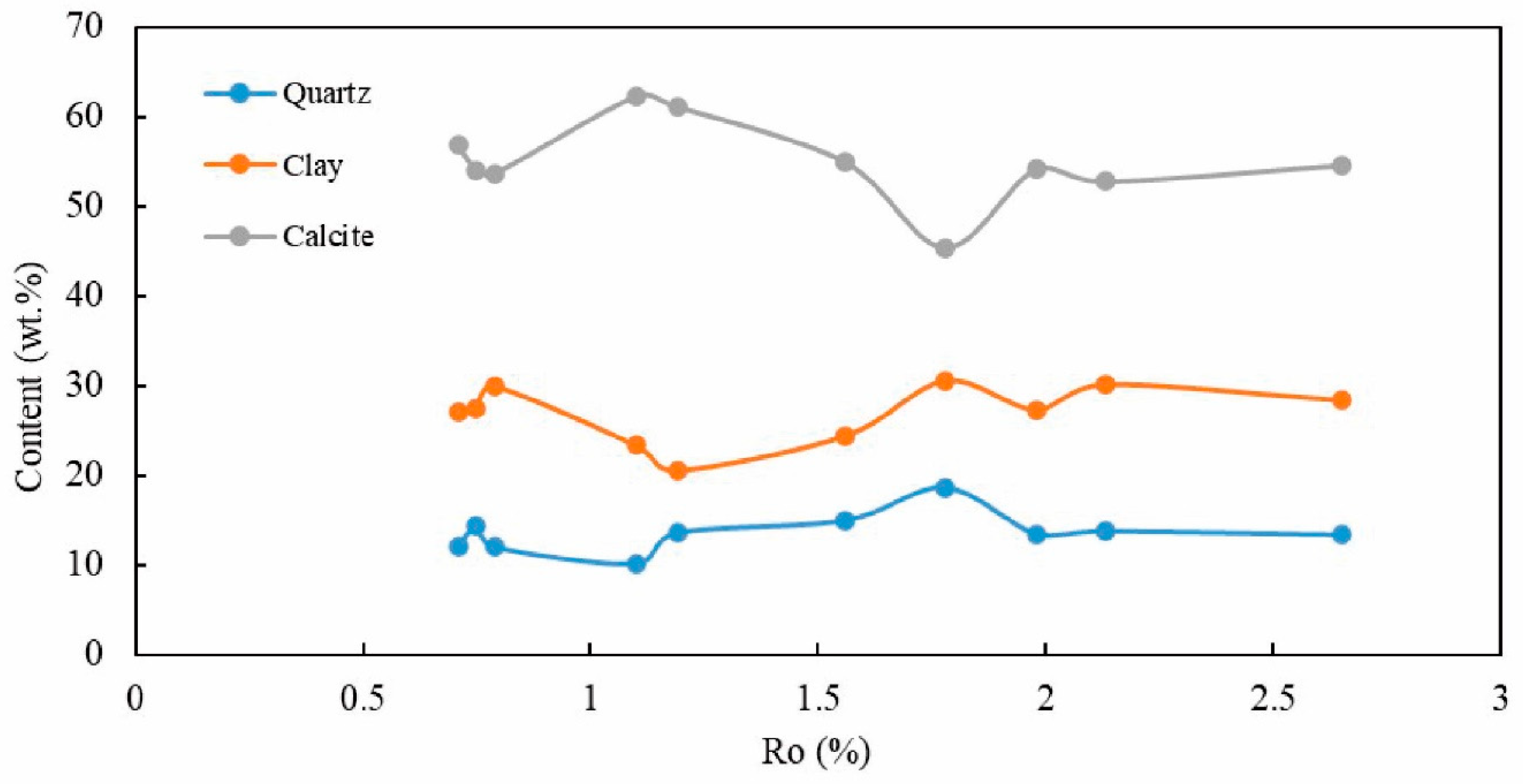
The samples were mainly composed of quartz, clay minerals and calcite, with the total amount of these three components being greater than 95% (Table 3). Calcite was the most dominant mineral at 45.4%–62.3%, followed by clay minerals at 20.6%–30.5% and quartz at 10.1%–18.7%. With the increase in thermal maturity, the calcite content first increased to the highest when Ro = 1.10%, then decreased to the lowest when Ro = 1.78%, and finally gradually increased. The trend of clay minerals content was opposite to that of calcite, and the quartz content is relatively stable (Figure 3).
4.3. Pore Volume and Structure Characterization
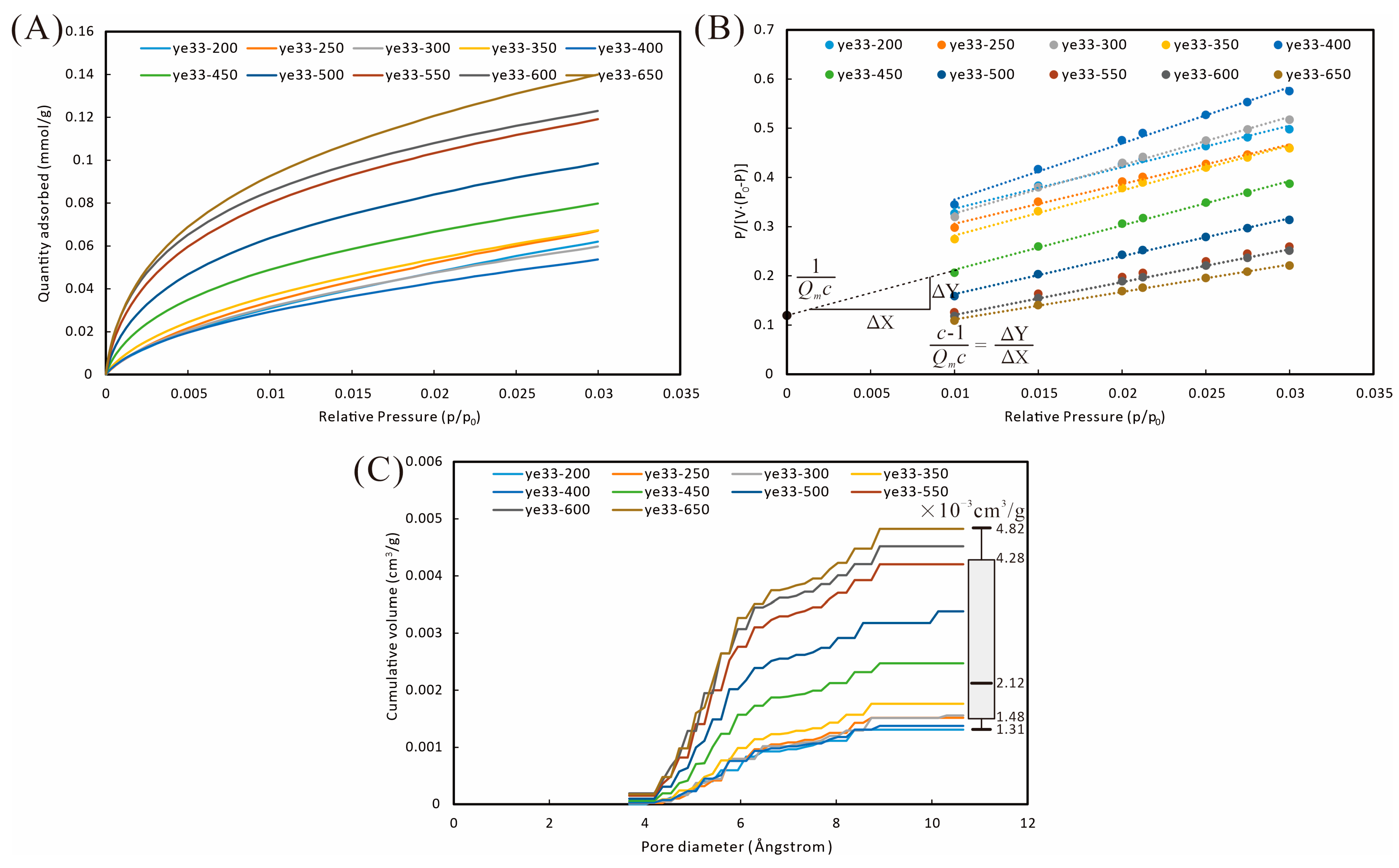
The CO2 adsorption capacity of 10 subsamples gradually increased with the relative pressure (P0/P), and the adsorption quantity was 0.054–0.140 mmol/g at P/P0 = 0.03 (P = 0.1 MPa), with ye33-650 (sample obtained from the artificial maturation experiment at a temperature of 650 °C) having the highest adsorption quantity (Figure 4A), according to the BET equation [12].
P is the balance pressure, MPa; P0 is the saturated vapor pressure of the adsorbent (CO2), MPa; Q is the actual adsorption quantity of the sample, mmol/g; Qm is the monolayer saturated adsorption quantity, mmol/g; and c is a constant related to the adsorption capacity.
Therefore, P/P0 has a linear relationship with based on Equation (1), which was a good fit for the 10 subsamples (Figure 4B). The Qm was 0.086–0.178 mmol/g, which reflected the sample’s specific surface area. The term c indicates the adsorption capacity of the samples, which was 34.5–124. The c of the 10 samples keeps increasing with an increasing maturity (Table 3), which represents a gradually increasing adsorption capacity, which may be the superposition of adsorption potential due to the increasing micropores (<2 nm) and pore surface complexity of the samples in the maturation process. The cumulative pore volumes (Figure 4C) of 0.36–1.06 nm micropores of the samples were calculated based on DFT theory [45] as 0.00131–0.0048 cm3/g.
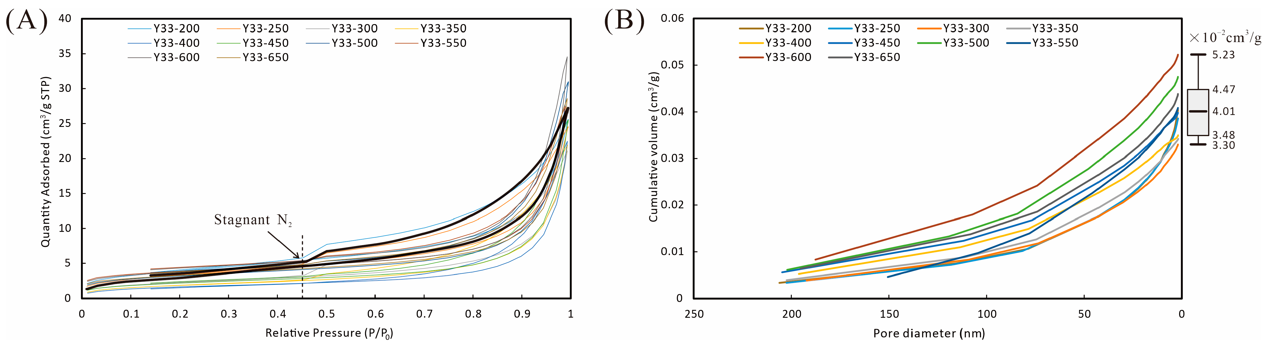
According to the IUPAC classification, the N2 adsorption-desorption curves of the sample belonged to type IV (Figure 5A), representing a porous medium rich in mesopores and micropores. The hysteresis loops and capillary condensation are the most typical features of type IV curves [46], and the hysteresis loop type is type H4, which was dominated by narrow-sized slit pores. Capillary condensation occurred at a P/P0 of 0.45–0.5, corresponding to a pore size of 3–4 nm. When the relative pressure was less than 0.45, a small quantity of nitrogen remained stagnant in the shales, indicating that the shales have a complex micro- and meso- (<4 nm) pore structure and matrix dissolution [47,48], with the stagnant quantity ranging from 0–0.73 cm3/g (Table 3) at standard temperature and pressure (STP, 273.15 K and 101.3 kPa). The cumulative pore volumes for 2–200 nm pore sizes were calculated from the BJH equation [23] as 0.033–0.052 cm3/g (Figure 5B).
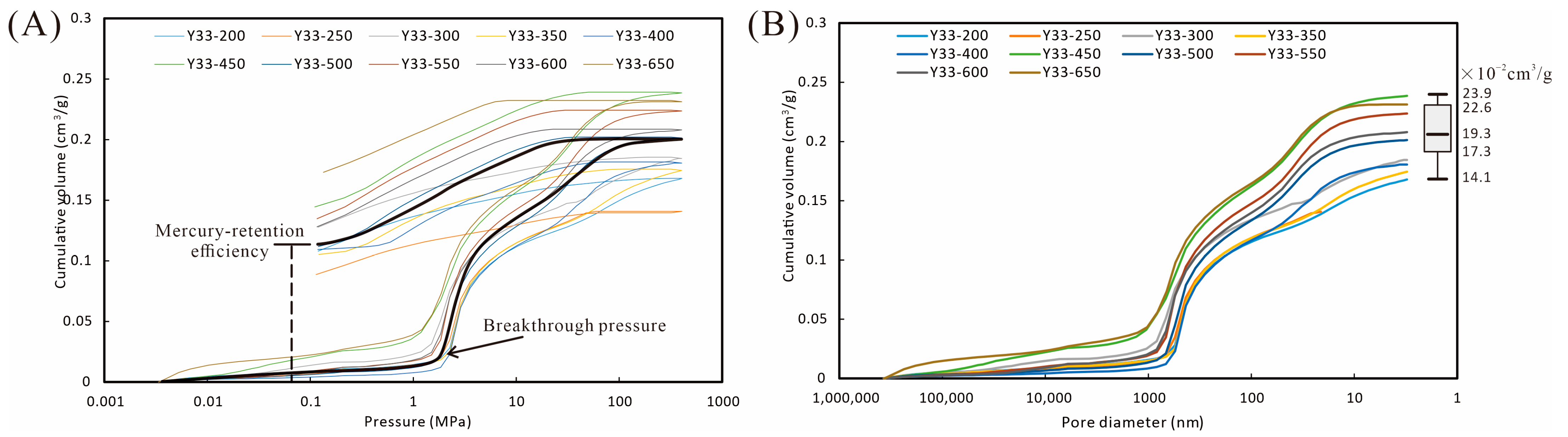
MIP has a wide pore-throat size characterization range [22,49]; the mercury intrusion curve increases slowly at pressures less than 1 MPa, the mercury intrusion volume increases rapidly when the pressure is higher than the breakthrough pressure, and then the mercury intrusion rate slows down as the pressure increases (Figure 6A). The maximum mercury intrusion volume of the samples varied widely, from 0.141 to 0.239 cm3/g. The mercury-extrusion curves were flat at high pressure (>40 MPa), followed by rapid mercury discharge from the sample. After the pressure was reduced to atmospheric pressure (101 kPa), there was still a large amount of mercury that could not be discharged, and the mercury retention efficiency was as large as 55.5%–74.8% (Table 3). The high mercury retention efficiency represents mercury retained in shale samples with poor sample pore connectivity and a large number of single-channel pores. The cumulative pore volumes of 3 nm–300 µm pore-throat sizes were calculated (Figure 6B) based on the Young–Dupre equation, the Washburn equation and the cylindrical pore assumption [39], but the irreversible destruction of pores by high-pressure intrusion may lead to the destruction of tiny pores and unreliable results less than 50 nm.
With the increase in Ro, the c value and adsorption capacity of the shale increased; the mercury retention efficiency gradually increased, representing that the pore structure became more complex; the breakthrough pressure decreased, indicating that the pore size of macropores grew larger (Table 4).
4.4. Pore Characteristics from SEM Imaging
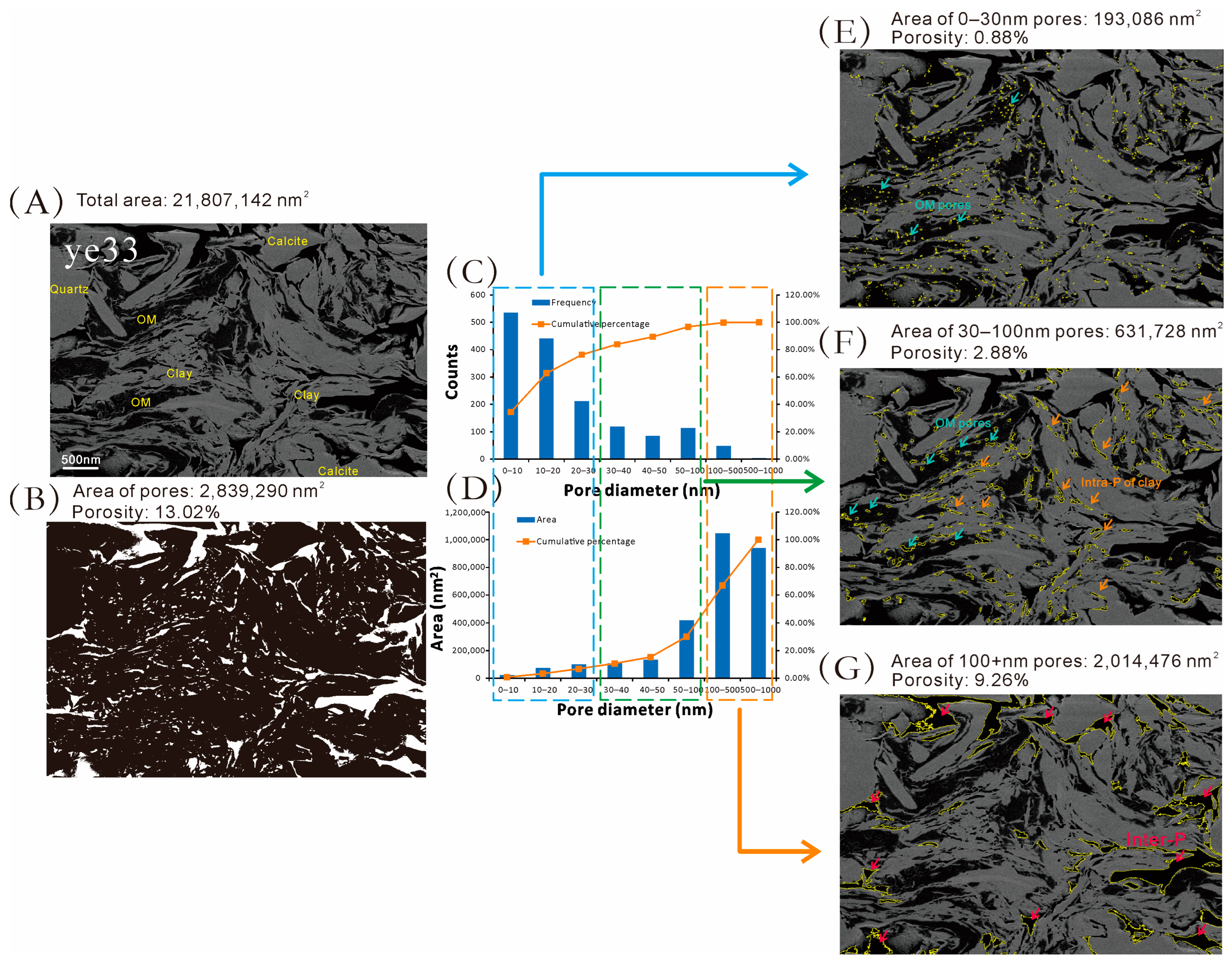
The morphology of minerals, OM, and pores of ye33 were observed at 20 k times and 0.2 kV (Figure 7A). The rigid minerals (quartz and calcite) are off-white and granular in the image, with clean surfaces and a few Intra-P. The clay minerals are narrow lamellar, with slit interlayer pores inside. The organic matter was dark and amorphous, with round and oval pores commonly found inside its particles. The size of Inter-P was larger than that of the other pores. Based on the pore processing (Figure 7B) and statistical results (Figure 7C,D), the original ye33 sample had a plane porosity of 13.02%, representing medium compaction [36]. Less than 30 nm pores were round and elliptical and are mainly distributed in organic matter and clay; the count accounted for 76.33% but only provided 0.88% porosity (Figure 7E). The 30–100 nm pores were mostly in the form of narrow slits, dominated by Intra-P of clay minerals, providing 2.88% porosity (Figure 7D). Pores larger than 100 nm were irregularly shaped, and most of them were Inter-P, providing 9.26% porosity.
5. Discussion
5.1. Pore-Size Polarization during Thermal Maturation
5.1.1. Evidence from SEM and IRT
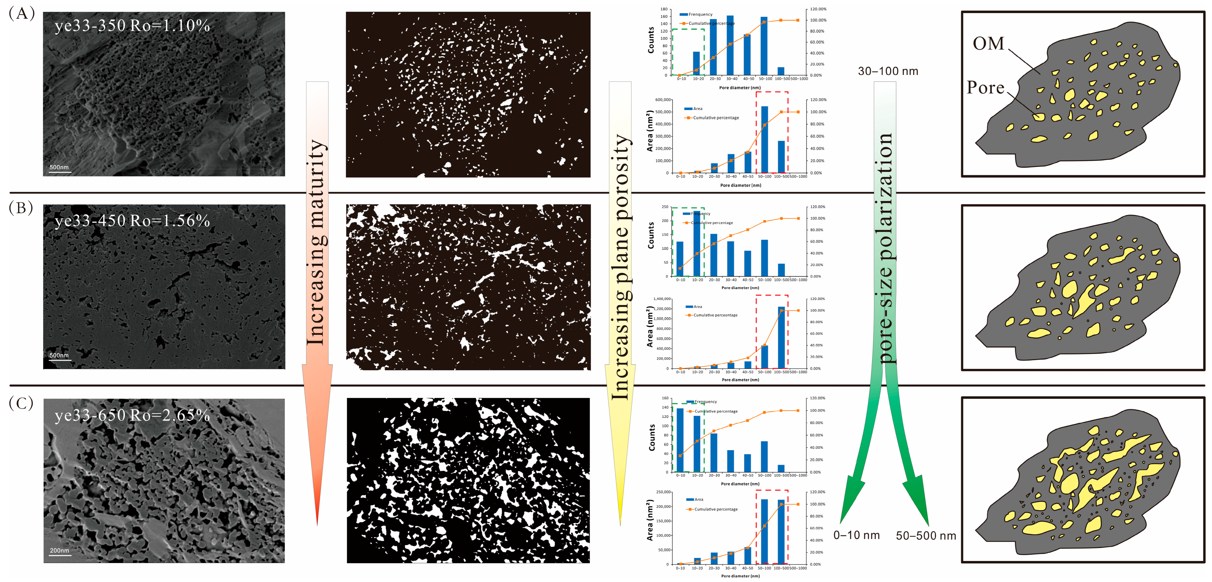
OM pores are formed inside or around OM during thermal maturation due to mass and density reduction and volume contraction in the process of hydrocarbon generation [50,51]. The gas genetic pores inside OM were round and elliptical in the image. Through comparative analyses of OM pore recognition results of samples with different maturities (Figure 8), under the same magnification, it was found that when Ro = 1.1%, the number of intra-OM pores mainly existed in two peaks of 30–40 nm and 50–100 nm in diameters, and the most pore volume was provided by 50–100 nm pores (accounting for 44.62%). A total of 672 pores were recognized, and the plane porosity was 5.67% (Figure 8A). When Ro increased to 1.56%, more tiny OM pores were generated, and the number peaks shifted down to 10–20 nm and 50–100 nm, respectively, while the most pore volume was provided by 100–500 nm pores (accounting for 59.34%). In addition, a total of 910 pores were recognized, and the plane porosity was 9.57% (Figure 8B). When Ro was further increased to 2.65%, some pores continued to expand and connect together, the number peaks changed to 0–10 nm and 50–100 nm, and its main pore volume was provided by 50–500 nm pores (accounting for 72.25%). Furthermore, a total of 514 pores were recognized, and the total plane porosity was 18.21% (Figure 8C). As a whole, the plane porosity of the intra-OM pores increases with an increasing maturity, generating more micropores and mesopores. Adjacent gas genetic pores were interconnected and merged into larger pores while generating more tiny pores in residual organic matter. These two effects cause polarization in the pore-size distribution of organic matter.
In low magnification and a large field of view of SEM imaging, the surrounding pores of OM and Intra-P and Inter-P of minerals were observed (Figure 9). The Intra-P and Inter-P of clay minerals are always dominated by slit-shaped pores with an increasing thermal maturation, which was closely related to the lamellar structure of clays [52]; however, the pores are widened, which may be related to hydrocarbon expulsion. Regardless of the maturation stage, the surfaces of rigid minerals (e.g., quartz, calcite, dolomite) are clean, with only a few dissolved pores and fractures, providing negligible pore volume (Figure 9A). The same phenomenon of polarization of pore sizes at 50–100 nm with increasing maturity was found at low magnification, with the formation of pores smaller than 10 nm and more pores larger than 100 nm (Figure 9B,D). At the over-maturation stage, large shrinkage fractures formed at the surrounding edge of the OM. The 100+ nm pores in ye33-650 were dominated by OM shrinkage fractures (Figure 9C), which was different from the original sample (ye33), where the 100+ pores were dominated by Inter-P (Figure 7D,G).
5.1.2. Evidence from LTGA and MIP
Based on the different methods and associated observational scales [53], the whole pore-size volume distributions of samples with different maturities were characterized (micropores from CO2 adsorption, mesopores from N2 adsorption, and macropores from MIP). At a maturity of less than 1.10%, there was only one peak in the pore-size volume distribution, and 100–1000 nm pores dominate (Figure 10), which is also consistent with our SEM observations of the original sample when the pore volume was mainly provided by intergranular pores. When Ro reached 1.19%, a second peak appeared in the 30–100 nm range, proving that the increase in pore space in this range corresponds to the increase in pores inside OM and pores of clay minerals. When Ro further increased to 1.56%, the volume of less than 2 nm pores and greater than 1000 nm pores increased, corresponding to the formation of micropores and surrounding shrinkage fractures of OM. Ultimately, there are four peaks (0–2, 30–100, 500–1000 nm, and 10–100 µm) in the whole pore-size volume distribution (Figure 10).
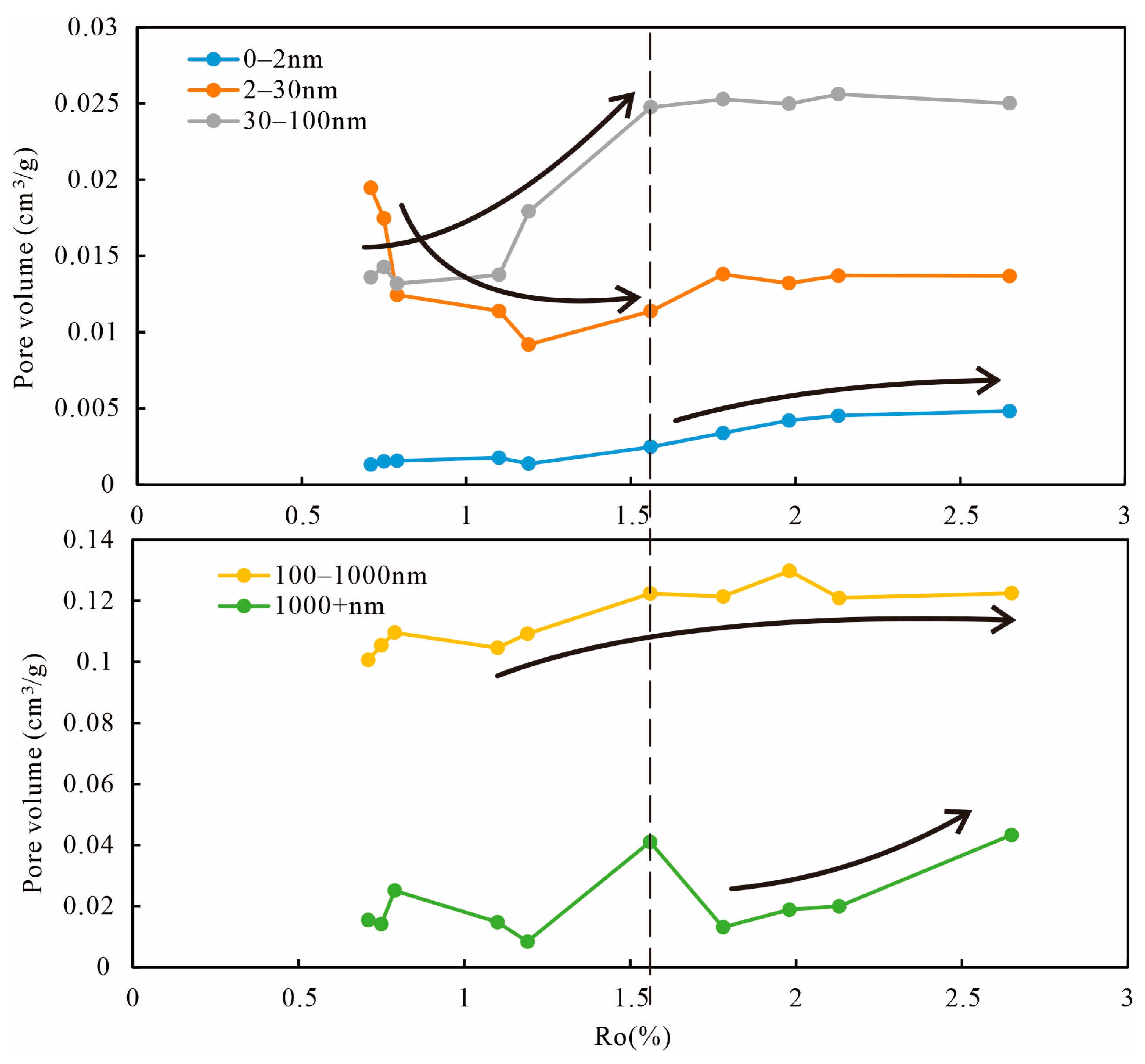
Along the increasing temperature and maturation levels, there are different changing patterns of pore development for the following five pore-size intervals (Figure 11): 0–2 nm pores increase continuously with the increase of Ro; 2–30 nm pores decrease first and reach the minimum at Ro = 1.19%, then gradually increase; 30–100 nm pores increase rapidly at Ro = 1.10%~1.56%, then stabilize; 100–1000 nm pores increase with the increasing maturity; 1000+ nm pores fluctuate with Ro, and increase faster in the high over maturity stage (Ro > 1.78%). Therefore, the whole pore-size distribution of the shale also exhibits polarization, with pore volumes of 0–30 nm and 100+ nm gradually increasing after Ro exceeds 1.5%.
5.2. Effects of Hydrocarbon Generation and Diagenesis
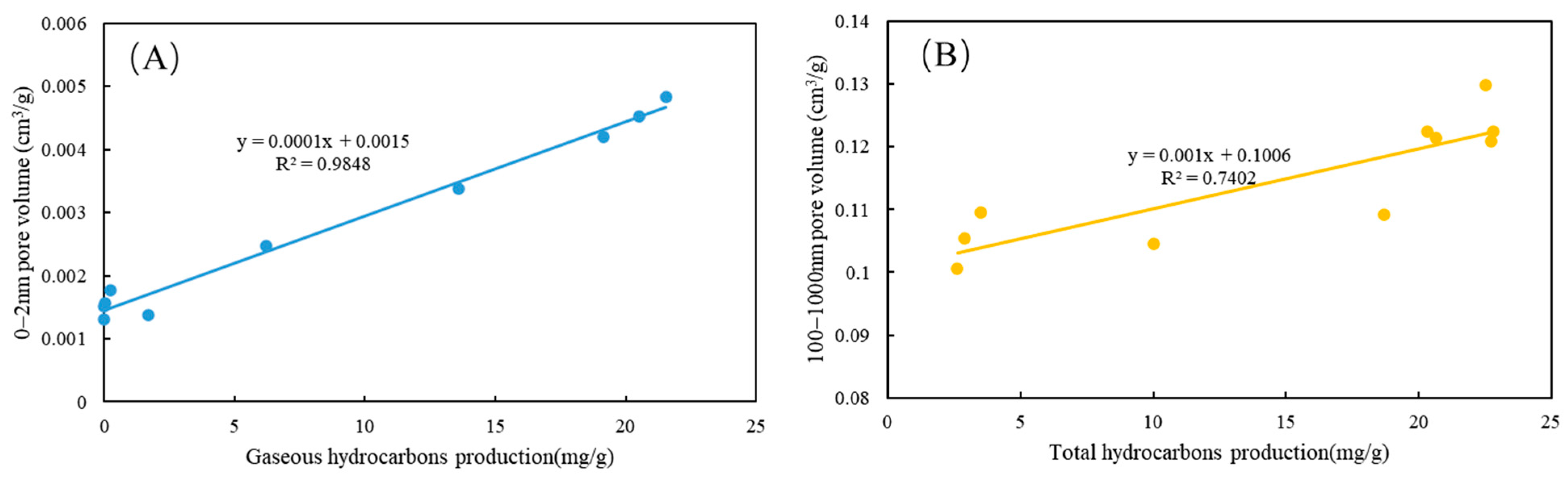
The results showed that the yield of hydrocarbons was closely related to the degree of pore development. The gaseous hydrocarbon yield had an extremely positive correlation with the volume of 0–2 nm pores (Figure 12A), representing micropore-level pores in organic matter produced by the generation and expulsion of small molecule hydrocarbons. Due to quality conservation, OM shrank to form macropores and fractures as the total hydrocarbon yield increased and 100–1000 nm pores increased (Figure 12B).
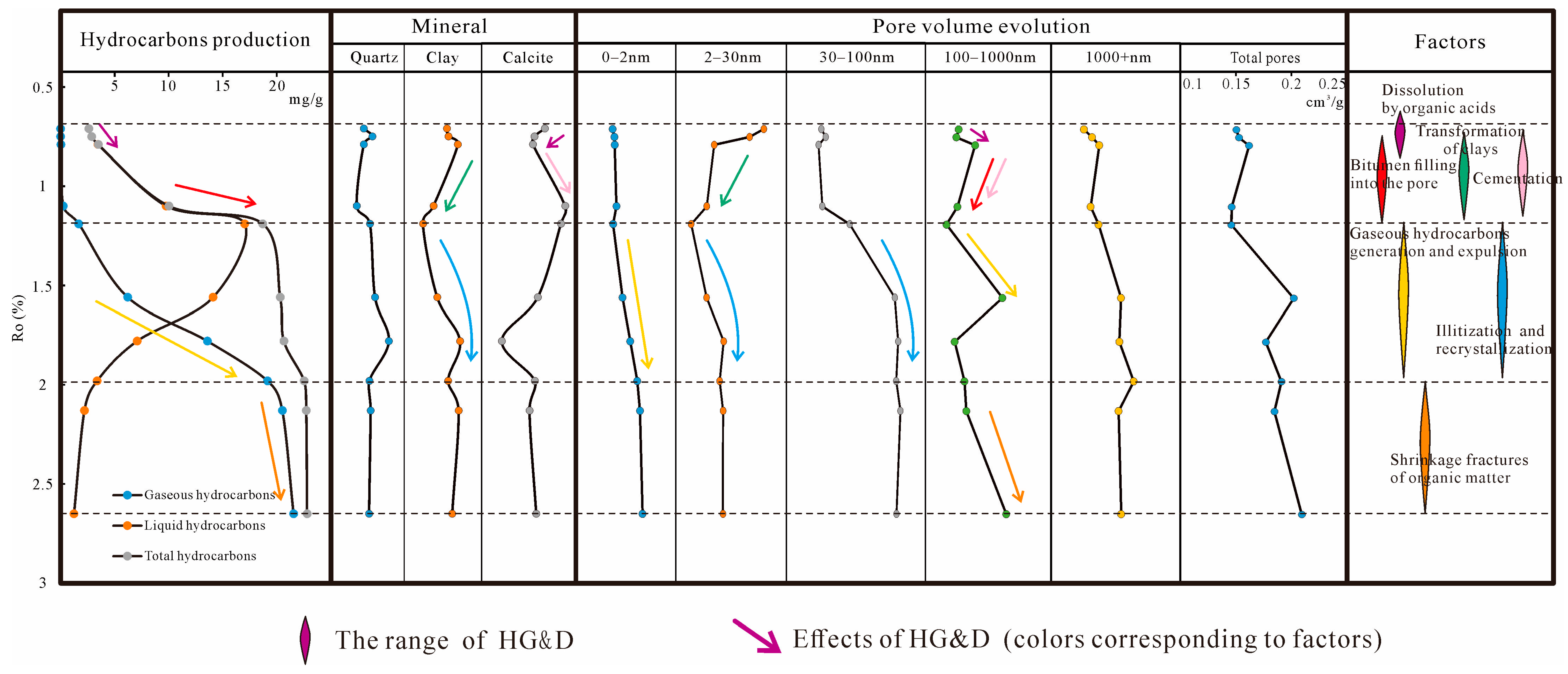
Based on the characteristics of HG&D and pore evolution, the evolution of organic-rich shale was divided into the following three stages (Figure 13):
- (1)
- Ro at 0.7%–1.2%, in the initial stage, kerogen decarboxylated and formed organic acids [54], calcite was dissolved in the acidic environment, and the Inter-P (100–1000 nm) increased. Subsequently, high-calcium fluids were redeposited in the Inter-P to produce calcium cementation [55], resulting in a decrease in Inter-P (100–1000 nm). The space of loose clay minerals (mainly kaolinite) is compressed, leading to a reduction in the Intra-P of clay minerals (2–30 nm). As the OM matures, the OM begins to generate large amounts of liquid hydrocarbons and 30–100 nm OM inside pores (30–100 nm) [56,57]. However, the generated liquid hydrocarbons and bitumen entered and blocked the Inter-P [58,59], resulting in a large reduction of 100–1000 nm pores. Some microcrystalline authigenic quartz generation also has a negative effect on the pores [60,61].
- (2)
- At 1.2%–2.0%, many gaseous hydrocarbons were generated, bitumen and OM shrank, spongy pores were formed in OM [62,63], and the OM pore size started to polarize, generating a large number of micropores (<2 nm) and a large volume of macropores (100–1000 nm). Illitization and recrystallization [64,65] of clay minerals increased the Inter-P and Intra-P of clay minerals, while gaseous hydrocarbons entered the pores, and high fluid pressure made the pores of clay larger, so the volume of 30–100 nm pores increased considerably.
- (3)
- When Ro was higher than 2.0%, the yield of hydrocarbons gradually decreased, so the change in the 0–100 nm pore volume was small. Most hydrocarbons have been expelled, and the density of the reduced OM resembles a sponge, with many pores developed in it. The OM then continued to shrink, forming shrinkage fractures at the perimeter of the organic matter [29,66], resulting in a continuous increase in the 100–1000 nm pores.
In conclusion, hydrocarbon generation controls organic pore development, diagenesis controls inorganic pore development, and both jointly control the shale pore evolution process.
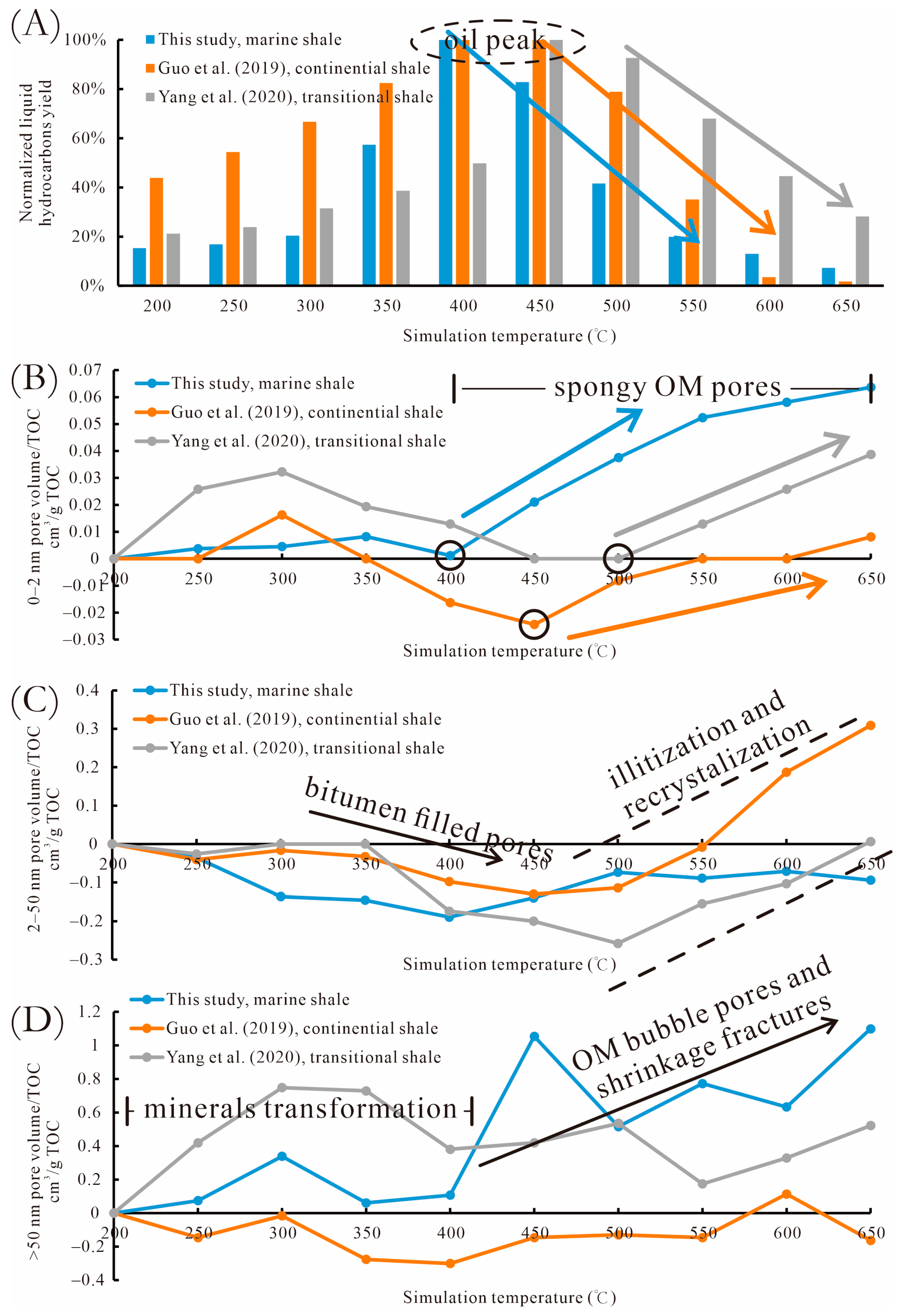
5.3. Compared to Continental and Transitional Shales
Upon categorizing the evolution of sample pores and analyzing the types of pores formed at various maturity stages, it was observed that as marine shale surpasses the oil generation peak (Ro > 1.2%), there is a noticeable rise in the overall pore volume across various pore sizes. This observation suggests a gradual enhancement in the reservoir’s porosity and permeability, thereby fostering favorable conditions for shale gas fracturing [67]. Comparison with published thermal simulation experiments-based pore evolution results [36] shows differences between marine, continental and transitional shales (Figure 14). Marine OM comprised of sapropel-rich organisms such as algae and foraminifera [68,69], which are more capable of oil production and earlier hydrocarbon production than the large amount of plant debris contained in the terrestrial and transitional phases [70,71,72]. In marine shales, a lot of pre-oil bitumen generates and fills the pores, resulting in a sudden drop in pore volume (e.g., mesopores). Marine shales also cross the oil production peak earlier, which, on the one hand, allows the organic matter pores to reappear [58], and on the other hand, new spongy organic matter [73,74] pore generation due to the cracking and degradation of organic matter (e.g., kerogen and pre-oil bitumen) into gaseous hydrocarbons. The micropores were more abundant in the marine shale after the oil peak, which was favorable to increase the specific surface area and methane adsorption in the future [75,76]. Prior to the oil peak, complex diagenesis (dissolution, cementation, replacement), clay mineral transformations (kaolinization, authigenic chlorite), and compositional differences (quartz origin, calcareous content, clay composition) complicated the macropores volume variation of the three shales [77,78]. Thus, differences in organic matter types and sedimentary mineral components were thought to dominate the differences in pore evolution among the three, which will require more abundant samples for detailed studies in the future. The findings of this study are constrained by the sample size. Moreover, the kerogen type present in the samples is classified as type II2 rather than type I, leading to notable disparities in the pore evolution process compared to certain marine strata. Additionally, the absence of investigation into various diagenetic processes during experimental design has resulted in unclear identification of influencing factors.
6. Conclusions
This study quantified shale pore evolution using IRT and SEM-assisted pore characterization experiments. The original triple classification of pores based on the pore scale was re-classified into six intervals (0–2, 2–30, 30–100, 100–1000, and 1000+ nm) based on the pore genesis. This classification helps to discuss and distinguish the specific effects of HG&D on pores at different scales during the thermal maturation processing of shales. Hydrocarbon generation was strongly correlated with 0–2 nm and 100–1000 nm pores, which was attributed to the polarization characteristics of OM-hosted pores during thermal evolution observed in SEM. Diagenesis (e.g., dissolution, mineral transformation, illitization and cementation) affected 2–30 nm, 30–100 nm, and 100–1000 nm pores at different stages, respectively. In addition, the bitumen filling and formation of shrinkage fractures affected 100–1000 nm or even 1000+ nm pores. Further, we also explored some of the differences and reasons for the thermal simulation experiments-based pore evolution of marine shales from those of continental and transitional shales published in the past. This study serves as a reference for future studies of shale pore evolution and provides a basis for multi-scale studies of genetic pores, especially for the prediction of reservoir space and beneficial stages of shale oil and gas in the underground.
Author Contributions
Conceptualization, S.G.; methodology, S.G.; software, X.Y.; validation, Z.W.; formal analysis, X.Y.; investigation, X.Y.; resources, S.G.; data curation, S.G.; writing—original draft preparation, X.Y.; writing—review and editing, Z.W.; visualization, Z.W.; supervision, S.G.; project administration, S.G.; funding acquisition, S.G. All authors have read and agreed to the published version of the manuscript.
Funding
This study received support from the Ministry of Science and Technology of the People’s Republic of China (Grant No. 2016ZX05034) and the China Geological Survey (Grant No. 2023-QN01). Financial support from the China Scholarship Council (CSC) and American Association of Petroleum Geologists (AAPG) Grants-in-Aid are gratefully acknowledged.
Data Availability Statement
Data are contained within the article.
Acknowledgments
We would like to thank anonymous reviewers for their suggestions.
Conflicts of Interest
The authors declare no conflict of interest.
References
- Bai, L.; Liu, B.; Yang, J.; Tian, S.; Wang, B.; Huang, S. Differences in hydrocarbon composition of shale oils in different phase states from the Qingshankou Formation, Songliao Basin, as determined from fluorescence experiments. Front. Earth Sci. 2021, 15, 438–456. [Google Scholar] [CrossRef]
- Zhang, Y.; Hu, Q.; Long, S.; Zhao, J.; Peng, N.; Wang, H.; Lin, X.; Sun, M. Mineral-controlled nm-μm-scale pore structure of saline lacustrine shale in Qianjiang Depression, Jianghan Basin, China. Mar. Pet. Geol. 2019, 99, 347–354. [Google Scholar] [CrossRef]
- Owusu, E.B.; Tsegab, H.; Sum, C.W.; Padmanabhan, E. Organic geochemical analyses of the Belata black shale, Peninsular Malaysia; implications on their shale gas potential. J. Nat. Gas Sci. Eng. 2019, 69, 102945. [Google Scholar] [CrossRef]
- Tan, J.; Horsfield, B.; Fink, R.; Krooss, B.; Schulz, H.-M.; Rybacki, E.; Zhang, J.; Boreham, C.J.; Van Graas, G.; Tocher, B.A. Shale gas potential of the major marine shale formations in the Upper Yangtze Platform, south China, Part III: Mineralogical, lithofacial, petrophysical, and rock mechanical properties. Energy Fuels 2014, 28, 2322–2342. [Google Scholar] [CrossRef]
- Enomoto, C.B.; Hackley, P.C.; Valentine, B.J.; Rouse, W.A.; Dulong, F.T.; Lohr, C.D.; Hatcherian, J.J. Geologic Characterization of the Hydrocarbon Resource Potential of the Upper Cretaceous Tuscaloosa Marine Shale in Mississippi and Louisiana, USA; United States Geological Survey: Reston, VA, USA, 2017.
- Zou, C.; Zhu, R.; Chen, Z.-Q.; Ogg, J.G.; Wu, S.; Dong, D.; Qiu, Z.; Wang, Y.; Wang, L.; Lin, S. Organic-matter-rich shales of China. Earth-Sci. Rev. 2019, 189, 51–78. [Google Scholar] [CrossRef]
- Jarvie, D.M.; Hill, R.J.; Ruble, T.E.; Pollastro, R.M. Unconventional shale-gas systems: The Mississippian Barnett Shale of north-central Texas as one model for thermogenic shale-gas assessment. AAPG Bull. 2007, 91, 475–499. [Google Scholar] [CrossRef]
- Wang, Y.; Cheng, H.; Hu, Q.; Liu, L.; Hao, L. Diagenesis and pore evolution for various lithofacies of the Wufeng-Longmaxi shale, southern Sichuan Basin, China. Mar. Pet. Geol. 2021, 133, 105251. [Google Scholar] [CrossRef]
- Zhu, W.; Chen, Z.; Liu, K. A new meshless method to solve the two-phase thermo-hydro-mechanical multi-physical field coupling problems in shale reservoirs. J. Nat. Gas Sci. Eng. 2022, 105, 104683. [Google Scholar] [CrossRef]
- Chen, J.; Xiao, X. Evolution of nanoporosity in organic-rich shales during thermal maturation. Fuel 2014, 129, 173–181. [Google Scholar] [CrossRef]
- Sun, L.; Tuo, J.; Zhang, M.; Wu, C.; Wang, Z.; Zheng, Y. Formation and development of the pore structure in Chang 7 member oil-shale from Ordos Basin during organic matter evolution induced by hydrous pyrolysis. Fuel 2015, 158, 549–557. [Google Scholar] [CrossRef]
- Rouquerol, J.; Llewellyn, P.; Rouquerol, F. Is the BET equation applicable to microporous adsorbents. Stud. Surf. Sci. Catal. 2007, 160, 49–56. [Google Scholar]
- Loucks, R.G.; Reed, R.M.; Ruppel, S.C.; Jarvie, D.M. Morphology, genesis, and distribution of nanometer-scale pores in siliceous mudstones of the Mississippian Barnett Shale. J. Sediment. Res. 2009, 79, 848–861. [Google Scholar] [CrossRef]
- Chen, Z.; Liu, X.; Yang, J.; Little, E.; Zhou, Y. Deep learning-based method for SEM image segmentation in mineral characterization, an example from Duvernay Shale samples in Western Canada Sedimentary Basin. Comput. Geosci. 2020, 138, 104450. [Google Scholar] [CrossRef]
- Sun, M.; Zhang, L.; Hu, Q.; Pan, Z.; Yu, B.; Sun, L.; Bai, L.; Fu, H.; Zhang, Y.; Zhang, C. Multiscale connectivity characterization of marine shales in southern China by fluid intrusion, small-angle neutron scattering (SANS), and FIB-SEM. Mar. Pet. Geol. 2020, 112, 104101. [Google Scholar] [CrossRef]
- Tahmasebi, P.; Javadpour, F.; Sahimi, M. Three-dimensional stochastic characterization of shale SEM images. Transp. Porous Media 2015, 110, 521–531. [Google Scholar] [CrossRef]
- Yang, R.; He, S.; Yi, J.; Hu, Q. Nano-scale pore structure and fractal dimension of organic-rich Wufeng-Longmaxi shale from Jiaoshiba area, Sichuan Basin: Investigations using FE-SEM, gas adsorption and helium pycnometry. Mar. Pet. Geol. 2016, 70, 27–45. [Google Scholar] [CrossRef]
- Zhou, S.; Yan, G.; Xue, H.; Guo, W.; Li, X. 2D and 3D nanopore characterization of gas shale in Longmaxi formation based on FIB-SEM. Mar. Pet. Geol. 2016, 73, 174–180. [Google Scholar] [CrossRef]
- Bai, L.-H.; Liu, B.; Du, Y.-J.; Wang, B.-Y.; Tian, S.-S.; Wang, L.; Xue, Z.-Q. Distribution characteristics and oil mobility thresholds in lacustrine shale reservoir: Insights from N2 adsorption experiments on samples prior to and following hydrocarbon extraction. Pet. Sci. 2022, 19, 486–497. [Google Scholar] [CrossRef]
- Chalmers, G.R.; Bustin, R.M.; Power, I.M. Characterization of gas shale pore systems by porosimetry, pycnometry, surface area, and field emission scanning electron microscopy/transmission electron microscopy image analyses: Examples from the Barnett, Woodford, Haynesville, Marcellus, and Doig units. AAPG Bull. 2012, 96, 1099–1119. [Google Scholar]
- Dong, T.; Harris, N.B.; Ayranci, K.; Twemlow, C.E.; Nassichuk, B.R. Porosity characteristics of the Devonian Horn River shale, Canada: Insights from lithofacies classification and shale composition. Int. J. Coal Geol. 2015, 141, 74–90. [Google Scholar] [CrossRef]
- Gao, F.; Song, Y.; Li, Z.; Xiong, F.; Chen, L.; Zhang, X.; Chen, Z.; Moortgat, J. Quantitative characterization of pore connectivity using NMR and MIP: A case study of the Wangyinpu and Guanyintang shales in the Xiuwu basin, Southern China. Int. J. Coal Geol. 2018, 197, 53–65. [Google Scholar] [CrossRef]
- Li, Y.; Schieber, J.; Fan, T.; Wei, X. Pore characterization and shale facies analysis of the Ordovician-Silurian transition of northern Guizhou, South China: The controls of shale facies on pore distribution. Mar. Pet. Geol. 2018, 92, 697–718. [Google Scholar] [CrossRef]
- Connan, J. Time-temperature relation in oil genesis: Geologic notes. AAPG Bull. 1974, 58, 2516–2521. [Google Scholar]
- Waples, D.W. Time and temperature in petroleum formation: Application of Lopatin’s method to petroleum exploration: Reply. AAPG Bull. 1982, 66, 1152. [Google Scholar]
- Sweeney, J.J.; Burnham, A.K. Evaluation of a simple model of vitrinite reflectance based on chemical kinetics. AAPG Bull. 1990, 74, 1559–1570. [Google Scholar]
- Songtao, W.; Rukai, Z.; Jinggang, C.; Jingwei, C.; Bin, B.; Zhang, X.; Xu, J.; Desheng, Z.; Jianchang, Y.; Xiaohong, L. Characteristics of lacustrine shale porosity evolution, Triassic Chang 7 member, Ordos Basin, NW China. Pet. Explor. Dev. 2015, 42, 185–195. [Google Scholar]
- Wang, F.; Guo, S. Influential factors and model of shale pore evolution: A case study of a continental shale from the Ordos Basin. Mar. Pet. Geol. 2019, 102, 271–282. [Google Scholar] [CrossRef]
- Guo, S.; Mao, W. Division of diagenesis and pore evolution of a Permian Shanxi shale in the Ordos Basin, China. J. Pet. Sci. Eng. 2019, 182, 106351. [Google Scholar] [CrossRef]
- Doveton, J.; Merriam, D. Borehole petrophysical chemostratigraphy of Pennsylvanian black shales in the Kansas subsurface. Chem. Geol. 2004, 206, 249–258. [Google Scholar] [CrossRef]
- Hakes, W.G. Trace Fossils from Brackish-Marine Shales, Upper Pennsylvanian of Kansas, USA; SEPM Society for Sedimentary Geology: Tulsa, OK, USA, 1984. [Google Scholar]
- Curtis, M.E.; Cardott, B.J.; Sondergeld, C.H.; Rai, C.S. Development of organic porosity in the Woodford Shale with increasing thermal maturity. Int. J. Coal Geol. 2012, 103, 26–31. [Google Scholar] [CrossRef]
- Dong, T.; Harris, N.B. The effect of thermal maturity on porosity development in the Upper Devonian–Lower Mississippian Woodford Shale, Permian Basin, US: Insights into the role of silica nanospheres and microcrystalline quartz on porosity preservation. Int. J. Coal Geol. 2020, 217, 103346. [Google Scholar] [CrossRef]
- Kibria, M.G.; Hu, Q.; Liu, H.; Zhang, Y.; Kang, J. Pore structure, wettability, and spontaneous imbibition of Woodford shale, Permian Basin, West Texas. Mar. Pet. Geol. 2018, 91, 735–748. [Google Scholar] [CrossRef]
- Jia, B.; Xian, C.; Tsau, J.-S.; Zuo, X.; Jia, W. Status and Outlook of Oil Field Chemistry-Assisted Analysis during the Energy Transition Period. Energy Fuels 2022, 36, 12917–12945. [Google Scholar] [CrossRef]
- Yang, X.G.; Guo, S.B. Porosity model and pore evolution of transitional shales: An example from the Southern North China Basin. Pet. Sci. 2020, 17, 1512–1526. [Google Scholar] [CrossRef]
- Clarkson, C.R.; Solano, N.; Bustin, R.M.; Bustin, A.; Chalmers, G.R.; He, L.; Melnichenko, Y.B.; Radliński, A.; Blach, T.P. Pore structure characterization of North American shale gas reservoirs using USANS/SANS, gas adsorption, and mercury intrusion. Fuel 2013, 103, 606–616. [Google Scholar] [CrossRef]
- Mastalerz, M.; Schimmelmann, A.; Drobniak, A.; Chen, Y. Porosity of Devonian and Mississippian New Albany Shale across a maturation gradient: Insights from organic petrology, gas adsorption, and mercury intrusion. AAPG Bull. 2013, 97, 1621–1643. [Google Scholar] [CrossRef]
- Drummond, C.; Israelachvili, J. Surface forces and wettability. J. Pet. Sci. Eng. 2002, 33, 123–133. [Google Scholar] [CrossRef]
- Washburn, E.W. The dynamics of capillary flow. Phys. Rev. 1921, 17, 273. [Google Scholar] [CrossRef]
- Choma, J.; Jaroniec, M.; Kloske, M. Improved pore-size analysis of carbonaceous adsorbents. Adsorpt. Sci. Technol. 2002, 20, 307–315. [Google Scholar] [CrossRef]
- Tian, S.; Bowen, L.; Liu, B.; Zeng, F.; Xue, H.; Erastova, V.; Greenwell, H.C.; Dong, Z.; Zhao, R.; Liu, J. A method for automatic shale porosity quantification using an Edge-Threshold Automatic Processing (ETAP) technique. Fuel 2021, 304, 121319. [Google Scholar] [CrossRef]
- Schneider, C.A.; Rasband, W.S.; Eliceiri, K.W. NIH Image to ImageJ: 25 years of image analysis. Nat. Methods 2012, 9, 671–675. [Google Scholar] [CrossRef]
- Kapur, J.N.; Sahoo, P.K.; Wong, A.K. A new method for gray-level picture thresholding using the entropy of the histogram. Comput. Vis. Graph. Image Process. 1985, 29, 273–285. [Google Scholar] [CrossRef]
- Lastoskie, C.; Gubbins, K.E.; Quirke, N. Pore size heterogeneity and the carbon slit pore: A density functional theory model. Langmuir 1993, 9, 2693–2702. [Google Scholar] [CrossRef]
- Li, Y.; Wang, Z.; Pan, Z.; Niu, X.; Yu, Y.; Meng, S. Pore structure and its fractal dimensions of transitional shale: A cross-section from east margin of the Ordos Basin, China. Fuel 2019, 241, 417–431. [Google Scholar] [CrossRef]
- Gregg, S. Studies in Surface Science and Catalysis; Elsevier: Amsterdam, The Netherlands, 1982; Volume 10, pp. 153–164. [Google Scholar]
- Yang, F.; Ning, Z.; Liu, H. Fractal characteristics of shales from a shale gas reservoir in the Sichuan Basin, China. Fuel 2014, 115, 378–384. [Google Scholar] [CrossRef]
- Al Hinai, A.; Rezaee, R.; Esteban, L.; Labani, M. Comparisons of pore size distribution: A case from the Western Australian gas shale formations. J. Unconv. Oil Gas Resour. 2014, 8, 1–13. [Google Scholar] [CrossRef]
- Borjigin, T.; Longfei, L.; Lingjie, Y.; Zhang, W.; Anyang, P.; Baojian, S.; Ye, W.; Yunfeng, Y.; Zhiwei, G. Formation, preservation and connectivity control of organic pores in shale. Pet. Explor. Dev. 2021, 48, 798–812. [Google Scholar] [CrossRef]
- Zhang, K.; Peng, J.; Wang, X.; Jiang, Z.; Song, Y.; Jiang, L.; Jiang, S.; Xue, Z.; Wen, M.; Li, X. Effect of organic maturity on shale gas genesis and pores development: A case study on marine shale in the upper Yangtze region, South China. Open Geosci. 2020, 12, 1617–1629. [Google Scholar] [CrossRef]
- Chen, S.; Han, Y.; Fu, C.; Zhu, Y.; Zuo, Z. Micro and nano-size pores of clay minerals in shale reservoirs: Implication for the accumulation of shale gas. Sediment. Geol. 2016, 342, 180–190. [Google Scholar] [CrossRef]
- Yang, X.; Guo, S. Comparative analysis of shale pore size characterization methods. Pet. Sci. Technol. 2020, 38, 793–799. [Google Scholar] [CrossRef]
- Nie, H.; Sun, C.; Liu, G.; Du, W.; He, Z. Dissolution pore types of the Wufeng Formation and the Longmaxi Formation in the Sichuan Basin, south China: Implications for shale gas enrichment. Mar. Pet. Geol. 2019, 101, 243–251. [Google Scholar] [CrossRef]
- Liu, H.; Zhang, S.; Song, G.; Xuejun, W.; Teng, J.; Wang, M.; Bao, Y.; Yao, S.; Wang, W.; Zhang, S. Effect of shale diagenesis on pores and storage capacity in the Paleogene Shahejie Formation, Dongying Depression, Bohai Bay Basin, east China. Mar. Pet. Geol. 2019, 103, 738–752. [Google Scholar] [CrossRef]
- Bernard, S.; Horsfield, B.; Schulz, H.-M.; Wirth, R.; Schreiber, A.; Sherwood, N. Geochemical evolution of organic-rich shales with increasing maturity: A STXM and TEM study of the Posidonia Shale (Lower Toarcian, northern Germany). Mar. Pet. Geol. 2012, 31, 70–89. [Google Scholar] [CrossRef]
- Loucks, R.G.; Reed, R.M.; Ruppel, S.C.; Hammes, U. Spectrum of pore types and networks in mudrocks and a descriptive classification for matrix-related mudrock pores. AAPG Bull. 2012, 96, 1071–1098. [Google Scholar] [CrossRef]
- Löhr, S.; Baruch, E.; Hall, P.; Kennedy, M. Is organic pore development in gas shales influenced by the primary porosity and structure of thermally immature organic matter? Org. Geochem. 2015, 87, 119–132. [Google Scholar] [CrossRef]
- Wei, L.; Mastalerz, M.; Schimmelmann, A.; Chen, Y. Influence of Soxhlet-extractable bitumen and oil on porosity in thermally maturing organic-rich shales. Int. J. Coal Geol. 2014, 132, 38–50. [Google Scholar] [CrossRef]
- Emmings, J.F.; Dowey, P.J.; Taylor, K.G.; Davies, S.J.; Vane, C.H.; Moss-Hayes, V.; Rushton, J.C. Origin and implications of early diagenetic quartz in the Mississippian Bowland Shale Formation, Craven Basin, UK. Mar. Pet. Geol. 2020, 120, 104567. [Google Scholar] [CrossRef]
- van de Kamp, P.C. Smectite-illite-muscovite transformations, quartz dissolution, and silica release in shales. Clay Clay Miner. 2008, 56, 66–81. [Google Scholar] [CrossRef]
- Huo, Z.; Peng, J.; Zhang, J.; Tang, X.; Li, P.; Ding, J.; Li, Z.; Liu, Z.; Dong, Z.; Lei, Y. Factors influencing the development of diagenetic shrinkage macro-fractures in shale. J. Pet. Sci. Eng. 2019, 183, 106365. [Google Scholar] [CrossRef]
- Meng, Q.; Hao, F.; Tian, J. Origins of non-tectonic fractures in shale. Earth-Sci. Rev. 2021, 222, 103825. [Google Scholar] [CrossRef]
- Berger, G.; Lacharpagne, J.-C.; Velde, B.; Beaufort, D.; Lanson, B. Kinetic constraints on illitization reactions and the effects of organic diagenesis in sandstone/shale sequences. Appl. Geochem. 1997, 12, 23–35. [Google Scholar] [CrossRef]
- Cuadros, J. Modeling of smectite illitization in burial diagenesis environments. Geochim. Cosmochim. Acta 2006, 70, 4181–4195. [Google Scholar] [CrossRef]
- Guo, K.; Song, H.; Chen, X.; Du, X.; Zhong, L. Graphene oxide as an anti-shrinkage additive for resorcinol–formaldehyde composite aerogels. Phys. Chem. Chem. Phys. 2014, 16, 11603–11608. [Google Scholar] [CrossRef] [PubMed]
- Jia, B.; Xian, C.-G. Permeability measurement of the fracture-matrix system with 3D embedded discrete fracture model. Pet. Sci. 2022, 19, 1757–1765. [Google Scholar] [CrossRef]
- Murphy, K.R.; Stedmon, C.A.; Waite, T.D.; Ruiz, G.M. Distinguishing between terrestrial and autochthonous organic matter sources in marine environments using fluorescence spectroscopy. Mar. Chem. 2008, 108, 40–58. [Google Scholar] [CrossRef]
- Meilijson, A.; Finkelman-Torgeman, E.; Bialik, O.M.; Boudinot, F.G.; Steinberg, J.; Waldmann, N.D.; Benjamini, C.; Vinegar, H.; Makovsky, Y. Significance to hydrocarbon exploration of terrestrial organic matter introduced into deep marine systems: Insights from the lower Cretaceous in the Levant Basin. Mar. Pet. Geol. 2020, 122, 104671. [Google Scholar] [CrossRef]
- Agrawal, V.; Sharma, S. Molecular characterization of kerogen and its implications for determining hydrocarbon potential, organic matter sources and thermal maturity in Marcellus Shale. Fuel 2018, 228, 429–437. [Google Scholar] [CrossRef]
- Wang, G.-C.; Sun, M.-Z.; Gao, S.-F.; Tang, L. The origin, type and hydrocarbon generation potential of organic matter in a marine-continental transitional facies shale succession (Qaidam Basin, China). Sci. Rep. 2018, 8, 6568. [Google Scholar] [CrossRef]
- Xia, L.-W.; Cao, J.; Wang, M.; Mi, J.-L.; Wang, T.-T. A review of carbonates as hydrocarbon source rocks: Basic geochemistry and oil–gas generation. Pet. Sci. 2019, 16, 713–728. [Google Scholar] [CrossRef]
- Zhu, X.; Cai, J.; Wang, X.; Zhang, J.; Xu, J. Effects of organic components on the relationships between specific surface areas and organic matter in mudrocks. Int. J. Coal Geol. 2014, 133, 24–34. [Google Scholar] [CrossRef]
- Wu, J.; Liang, C.; Hu, Z.; Yang, R.; Xie, J.; Wang, R.; Zhao, J. Sedimentation mechanisms and enrichment of organic matter in the Ordovician Wufeng Formation-Silurian Longmaxi Formation in the Sichuan Basin. Mar. Pet. Geol. 2019, 101, 556–565. [Google Scholar] [CrossRef]
- Xiong, J.; Liu, X.; Liang, L.; Zeng, Q. Methane adsorption on carbon models of the organic matter of organic-rich shales. Energy Fuels 2017, 31, 1489–1501. [Google Scholar] [CrossRef]
- Zhang, T.; Ellis, G.S.; Ruppel, S.C.; Milliken, K.; Yang, R. Effect of organic-matter type and thermal maturity on methane adsorption in shale-gas systems. Org. Geochem. 2012, 47, 120–131. [Google Scholar] [CrossRef]
- Milliken, K.L.; Olson, T. Silica diagenesis, porosity evolution, and mechanical behavior in siliceous mudstones, Mowry Shale (Cretaceous), Rocky Mountains, USA. J. Sediment. Res. 2017, 87, 366–387. [Google Scholar] [CrossRef]
- Liang, C.; Cao, Y.; Liu, K.; Jiang, Z.; Wu, J.; Hao, F. Diagenetic variation at the lamina scale in lacustrine organic-rich shales: Implications for hydrocarbon migration and accumulation. Geochim. Cosmochim. Acta 2018, 229, 112–128. [Google Scholar] [CrossRef]
Figure 1.
(A) Sample location in Kansas; (B) stratigraphic position of the Upper Pennsylvanian black shale studied.
Figure 1.
(A) Sample location in Kansas; (B) stratigraphic position of the Upper Pennsylvanian black shale studied.
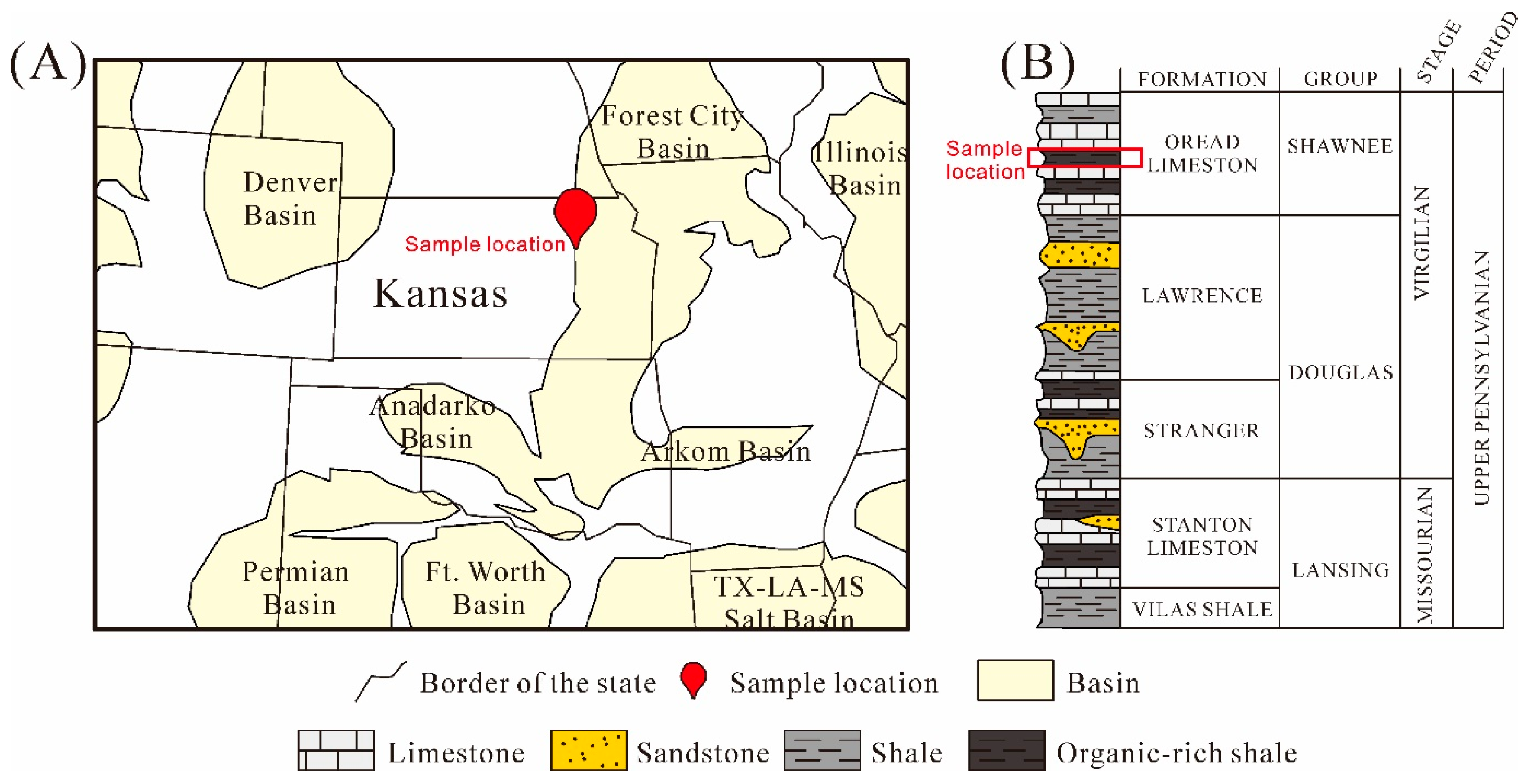
Figure 2.
Yields of hydrocarbons at different maturities from the thermal maturation experiments.
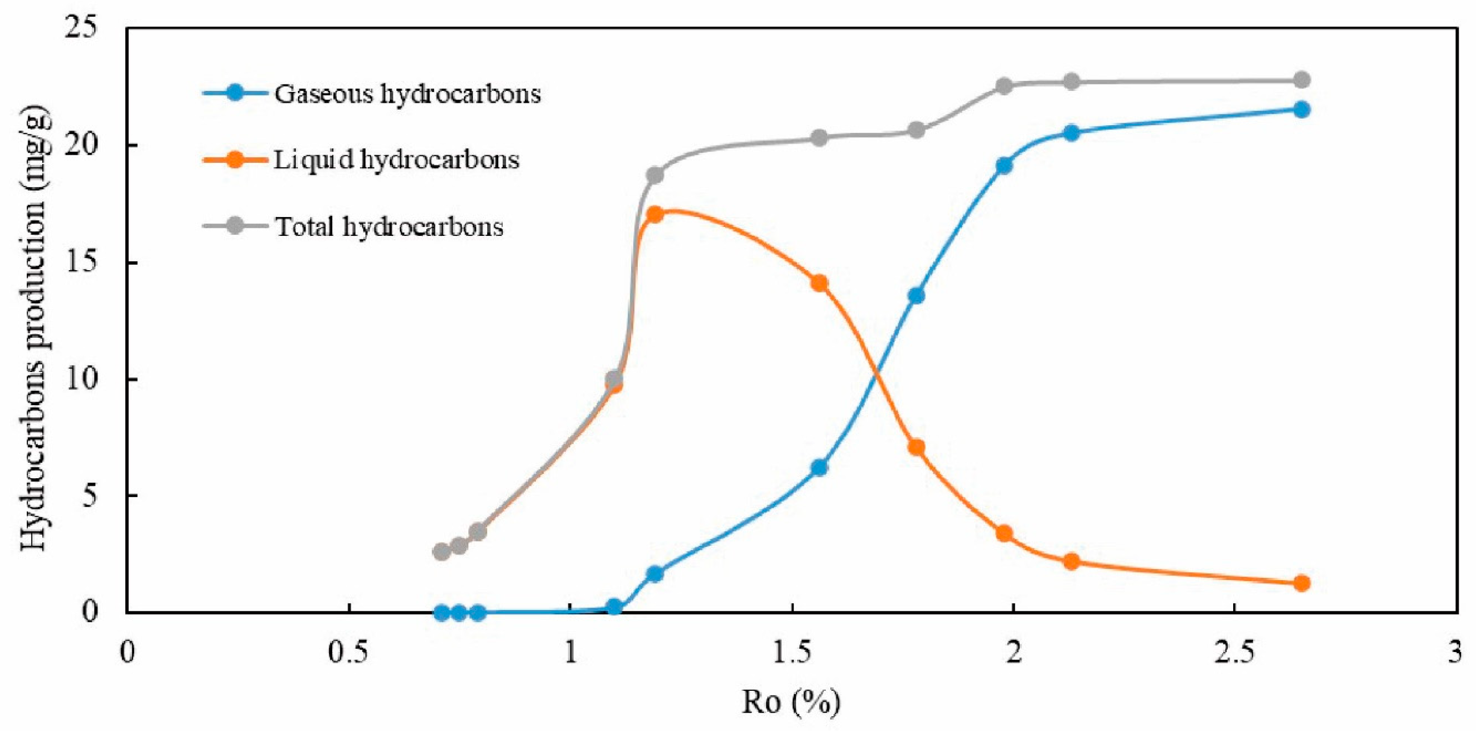
Figure 3.
Changes in the compositions of quartz, clays, and calcite at different maturities.

Figure 4.
Low-temperature CO2 adsorption curves (A), BET equation fitting results (B) and DFT cumulative pore volumes (C) for 10 subsamples.
Figure 4.
Low-temperature CO2 adsorption curves (A), BET equation fitting results (B) and DFT cumulative pore volumes (C) for 10 subsamples.

Figure 5.
Low-temperature N2 adsorption-desorption curves (A) and BJH cumulative pore volumes (B) for 10 subsamples.
Figure 5.
Low-temperature N2 adsorption-desorption curves (A) and BJH cumulative pore volumes (B) for 10 subsamples.

Figure 6.
Mercury intrusion-extrusion curves (A) and MIP cumulative pore volumes (B) for 10 subsamples.
Figure 6.
Mercury intrusion-extrusion curves (A) and MIP cumulative pore volumes (B) for 10 subsamples.

Figure 7.
(A) SEM image of the ye33 sample; (B) Binarized images for pore recognition; (C) Distribution of pore counts by statistics from (B); (D) distribution of pore volume by statistics from (B); (E) Features of pores in 0–30 nm, (F) Features of pores in 30–100 nm and (G) Features of pores in 100+ nm.

Figure 8.
Characterization, recognition, and distribution of pores inside OM of subsamples at the simulated temperatures of 350 °C (A), 450 °C (B) and 650 °C (C).
Figure 8.
Characterization, recognition, and distribution of pores inside OM of subsamples at the simulated temperatures of 350 °C (A), 450 °C (B) and 650 °C (C).

Figure 9.
(A) Characterization and distribution of the pores of the ye33-450 sample in a large field of view; (B) Characterization and distribution of the pores of the ye33-650 sample in a large field of view; (C) Recognition results and features of the 100+ nm pores of the ye33-650 sample; (D) Spongy OM pores and perimeter shrinkage fracture of the ye33-650 sample.
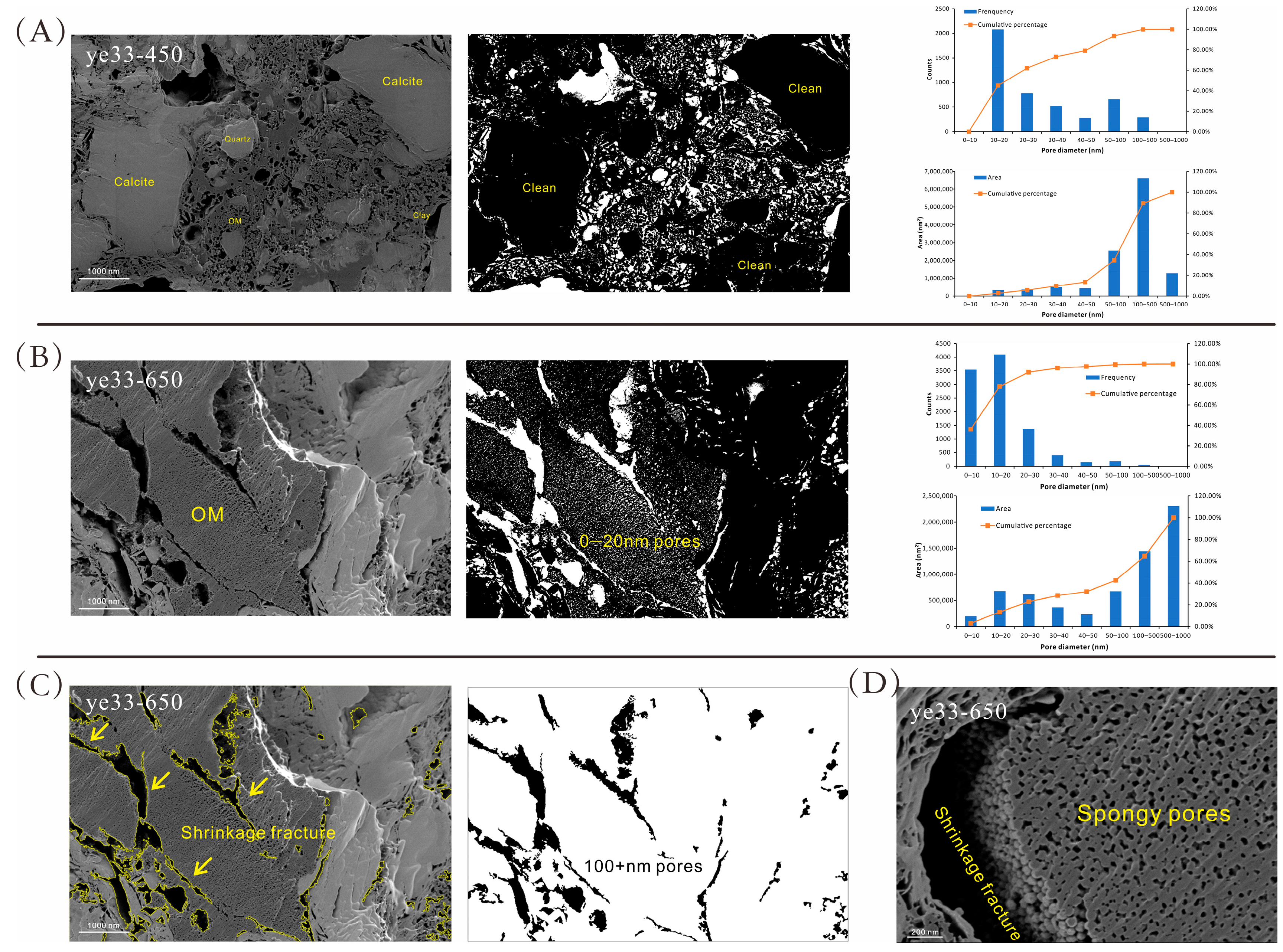
Figure 10.
Pore-size volume distribution of subsamples with different maturities. (Arrows represent new peaks generated compared to the previous stage).
Figure 10.
Pore-size volume distribution of subsamples with different maturities. (Arrows represent new peaks generated compared to the previous stage).
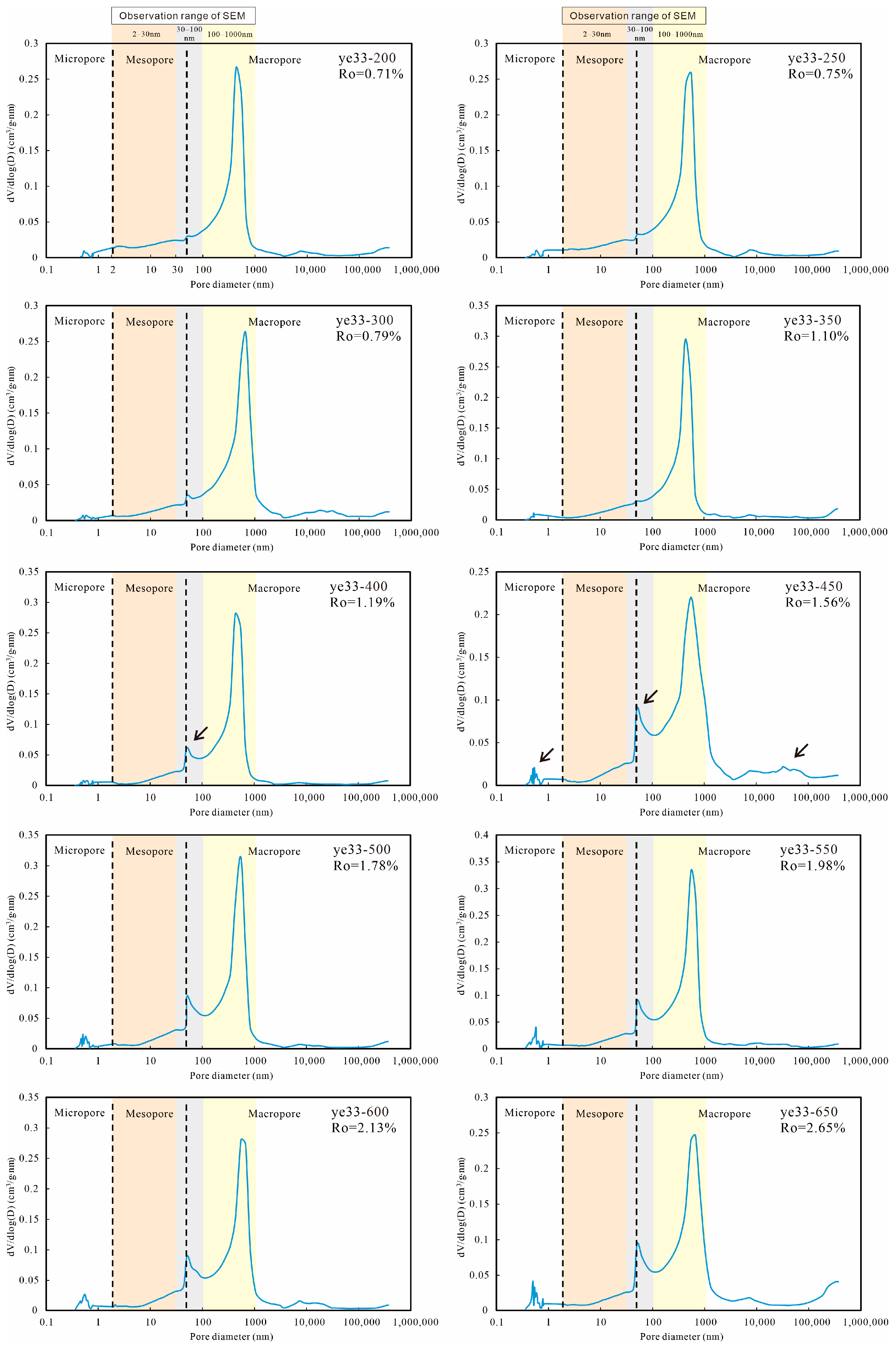
Figure 11.
Evolution of pore volume at different pore scales. (Arrows indicate the trend of pore volume variation with maturity at different scales).
Figure 11.
Evolution of pore volume at different pore scales. (Arrows indicate the trend of pore volume variation with maturity at different scales).

Figure 12.
(A) Correlation between 0–2 nm pores and the yield of gaseous hydrocarbons; (B) correlation between 100–1000 nm pores and the yield of total hydrocarbons.
Figure 12.
(A) Correlation between 0–2 nm pores and the yield of gaseous hydrocarbons; (B) correlation between 100–1000 nm pores and the yield of total hydrocarbons.

Figure 13.
Effects of HG&D on the evolution of pores of different sizes. (Arrows represent the changing trends of different curves).
Figure 13.
Effects of HG&D on the evolution of pores of different sizes. (Arrows represent the changing trends of different curves).

Figure 14.
Comparison of thermal simulation results for marine, continental and transitional shales (A) variation of normalized liquid hydrocarbon yield with simulation temperature (at oil peak, normalized liquid hydrocarbon yield = 1); (B) variation of 0–2 nm pore volume with simulation temperature; (C) variation of 2–50 nm pore volume with simulation temperature; (D) variation of >50 nm pore volume with simulation temperature [29,36].


Table 1.
Basic information of the original shale sample.
| Sample ID | Ro (%) | TOC (wt.%) | S2 (mg/g) | Kerogen Type |
|---|---|---|---|---|
| ye33 | 0.65 | 5.52 | 22.32 | II2 |
Table 2.
Ro and hydrocarbon yields of the simulated subsamples.
| Sample ID | Final Temperature | Ro | Gaseous Hydrocarbons | Liquid Hydrocarbons | Total Hydrocarbons |
|---|---|---|---|---|---|
| (°C) | (%) | mg/g | mg/g | mg/g | |
| ye33-200 | 200.0 | 0.71 | 0.00 | 2.62 | 2.62 |
| ye33-250 | 250.0 | 0.75 | 0.00 | 2.88 | 2.88 |
| ye33-300 | 300.0 | 0.79 | 0.03 | 3.47 | 3.50 |
| ye33-350 | 350.0 | 1.1 | 0.25 | 9.77 | 10.02 |
| ye33-400 | 400.0 | 1.19 | 1.68 | 17.02 | 18.70 |
| ye33-450 | 450.0 | 1.56 | 6.21 | 14.11 | 20.31 |
| ye33-500 | 500.0 | 1.78 | 13.57 | 7.08 | 20.65 |
| ye33-550 | 550.0 | 1.98 | 19.13 | 3.39 | 22.52 |
| ye33-600 | 600.0 | 2.13 | 20.51 | 2.21 | 22.72 |
| ye33-650 | 650.0 | 2.65 | 21.55 | 1.25 | 22.80 |
Table 3.
Whole-rock mineral composition by XRD analyses.
| Sample ID | Whole-Rock Mineral Content (%) | |||||||
|---|---|---|---|---|---|---|---|---|
| Clay | Quartz | Potassium Feldspar | Plagioclase | Calcite | Dolomite | Pyrite | Siderite | |
| ye33-200 | 27 | 12 | 0.4 | 1.7 | 56.9 | 0.9 | 0.4 | 0.7 |
| ye33-250 | 27.4 | 14.3 | 0.8 | 1.4 | 54.1 | 0.6 | 0.7 | 0.7 |
| ye33-300 | 29.9 | 12 | 0.5 | 1.3 | 53.7 | 1 | 0.7 | 0.9 |
| ye33-350 | 23.4 | 10.1 | 0.4 | 1.1 | 62.3 | 1.1 | 0.7 | 0.9 |
| ye33-400 | 20.6 | 13.6 | 0.8 | 1.6 | 61.2 | 1 | 0.3 | 0.9 |
| ye33-450 | 24.4 | 15 | 0.5 | 1.6 | 55 | 1.2 | 0.7 | 1.6 |
| ye33-500 | 30.5 | 18.7 | 0.9 | 1.4 | 45.4 | 1.8 | 0.3 | 1 |
| ye33-550 | 27.3 | 13.5 | 0.8 | 1.5 | 54.2 | 1.4 | 0.3 | 1 |
| ye33-600 | 30.1 | 13.8 | 0.5 | 1 | 52.8 | 0.8 | 0.1 | 0.9 |
| ye33-650 | 28.4 | 13.4 | 0.5 | 0.9 | 54.6 | 1 | 0.3 | 0.9 |
Table 4.
Statistics of key parameters of pore-size characterization methods.
| Scheme 2 | CO2 | N2 | MIP | |||||
|---|---|---|---|---|---|---|---|---|
| Qm (mmol/g) | c | Q (mmol/g) | Stagnant N2 (cm3/g STP) | Q (cm3/g STP) | Retention Efficiency (%) | Breakthrough Pressure (MPa) | Injection Volume (cm3/g) | |
| ye33-200 | 0.115 | 34.47 | 0.062 | 0.40 | 25.60 | 64.30 | 2.26 | 0.17 |
| ye33-250 | 0.121 | 36.74 | 0.067 | 0.29 | 24.54 | 62.94 | 2.26 | 0.14 |
| ye33-300 | 0.100 | 43.91 | 0.060 | 0.26 | 21.09 | 69.21 | 1.85 | 0.18 |
| ye33-350 | 0.107 | 48.98 | 0.067 | 0.12 | 21.95 | 60.27 | 2.27 | 0.17 |
| ye33-400 | 0.086 | 48.55 | 0.054 | 0.00 | 22.47 | 60.56 | 2.26 | 0.18 |
| ye33-450 | 0.109 | 74.80 | 0.080 | 0.26 | 25.52 | 60.57 | 1.19 | 0.24 |
| ye33-500 | 0.128 | 91.06 | 0.099 | 0.73 | 30.98 | 55.52 | 2.26 | 0.20 |
| ye33-550 | 0.149 | 107.64 | 0.119 | 0.70 | 27.48 | 60.26 | 1.85 | 0.22 |
| ye33-600 | 0.149 | 123.77 | 0.123 | 0.66 | 34.55 | 61.56 | 1.85 | 0.21 |
| ye33-650 | 0.178 | 100.48 | 0.140 | 0.57 | 28.61 | 74.82 | 1.53 | 0.23 |
Disclaimer/Publisher’s Note: The statements, opinions and data contained in all publications are solely those of the individual author(s) and contributor(s) and not of MDPI and/or the editor(s). MDPI and/or the editor(s) disclaim responsibility for any injury to people or property resulting from any ideas, methods, instructions or products referred to in the content. |
© 2024 by the authors. Licensee MDPI, Basel, Switzerland. This article is an open access article distributed under the terms and conditions of the Creative Commons Attribution (CC BY) license (https://creativecommons.org/licenses/by/4.0/).
Share and Cite
MDPI and ACS Style
Wang, Z.; Yang, X.; Guo, S. Evolution of Pore Spaces in Marine Organic-Rich Shale: Insights from Multi-Scale Analysis of a Permian–Pennsylvanian Sample. Minerals 2024, 14, 392. https://doi.org/10.3390/min14040392
AMA Style
Wang Z, Yang X, Guo S. Evolution of Pore Spaces in Marine Organic-Rich Shale: Insights from Multi-Scale Analysis of a Permian–Pennsylvanian Sample. Minerals. 2024; 14(4):392. https://doi.org/10.3390/min14040392
Chicago/Turabian StyleWang, Zilong, Xiaoguang Yang, and Shaobin Guo. 2024. "Evolution of Pore Spaces in Marine Organic-Rich Shale: Insights from Multi-Scale Analysis of a Permian–Pennsylvanian Sample" Minerals 14, no. 4: 392. https://doi.org/10.3390/min14040392
Note that from the first issue of 2016, this journal uses article numbers instead of page numbers. See further details here.