
Using Euler Deconvolution as Part of a Mineral Exploration Project

School of Geosciences, University of the Witwatersrand, Johannesburg 2050, South Africa
Minerals 2024, 14(4), 393; https://doi.org/10.3390/min14040393
Submission received: 8 March 2024
/
Revised: 5 April 2024
/
Accepted: 6 April 2024
/
Published: 10 April 2024
(This article belongs to the Section Mineral Exploration Methods and Applications)
Abstract
:Mineral exploration projects can make considerable use of a variety of geophysical techniques and datasets, including magnetic and gravity data. The interpretation of large quantities of data can be very time consuming, so semi-automatic interpretation techniques are often used to provide initial estimates of the parameters (primarily the location and depth) of the sources of anomalies. Euler deconvolution is a commonly used interpretation method for potential fields which has a number of advantages over many other techniques, such as working in the presence of remanent magnetisation, and not being restricted to a particular model such as a contact. A second-order version of Euler’s equation is introduced here, which is much less affected by trends in the data than the standard method and additionally produces depth parabolas, which simplify the interpretation of results. The method was applied to aeromagnetic data from a mineral exploration project in Southern Africa and provided plausible results.
1. Introduction
Mineral exploration projects can make considerable use of a variety of geophysical techniques, including magnetic and gravity data. The interpretation of large quantities of geophysical data can be very time consuming, so semi-automatic interpretation techniques are often used to provide initial estimates of the parameters (primarily the location and depth) of the sources of anomalies There are many semi-automatic interpretation techniques available, such as analytic-signal-amplitude-based methods [1,2,3,4], Werner deconvolution [5], source-distance approaches [6,7], and Euler deconvolution. Euler deconvolution is based on Euler’s homogenous function theorem, which is widely used throughout mathematics and physics. It states that for homogenous functions (i.e., those in which all terms are raised to the same power) of degree N, then [8,9,10,11]
f(t·x,t·z) = tNf(x,z)
Differentiating Equation (1) with respect to t, and then setting t = 1, provides
Note that Equation (2) basically states that function f can be written in terms of combinations of its first order derivatives. When applied to potential field data f, then x and z are interpreted as the distances (Δx and Δz) from the current point to the source in the x and z planes. The degree of homogeneity N (which is also termed the structural index, or SI) is the rate of decay of the amplitude of the field with distance from the source, e.g., N = 1 for the magnetic response of a dyke. Equation (2) is usually solved for Δx and Δz using a moving window of data points, with N being specified. The solutions are effectively averaged over the window size, so while larger window sizes can reduce the effect of random noise, they can result in the smearing of the solution’s horizontal location and can also make the results more sensitive to interference from adjacent anomalies. Sometimes a background field term B is subtracted from the field f, but Euler’s equation is only for single sources, which implies that (if necessary) this has already been done.
2. Materials and Methods
Derivatives of potential fields are also homogenous functions, so Euler deconvolution is frequently applied to them [14,15]
Applying Euler deconvolution to higher order derivatives of the field can reduce the sensitivity of the method to regional field and interference issues. Euler deconvolution can also be applied to combinations of the derivatives, such as the analytic signal amplitude [16] or the Tilt angle [17].
Substituting Equations (4) and (5) into Equation (2) provides the second-order Euler equation
Higher order equations can be generated in a similar manner. Using Laplace’s equation, then
Equation (7) is solved for (Δx2 − Δz2) and (2Δx·Δz) using a moving window of data points in the usual manner, then Δx and Δz are obtained by solving a quadratic equation, i.e., let a = (Δx2 − Δz2) and b = (2Δx·Δz), then
Similarly substituting Equations (4) and (5) into Equation (3) provides the Hilbert transform of Equation (7);
Note that the second-order equations do not have any first order derivative terms, which makes them less sensitive to the presence of linear regional fields than Equations (2) and (3). Additionally, as the depth of the source Δz = √−a when Δx = 0 (Equation (7)), plotting √−a yields a ‘depth parabola’, which is a useful check on the validity of the Euler solutions.
Equations (4)–(10) use second-order derivatives of the field, which naturally can make them sensitive to noise. If this is an issue, then either regularised derivatives [18] or upward continuation of the field can be used.
3. Results
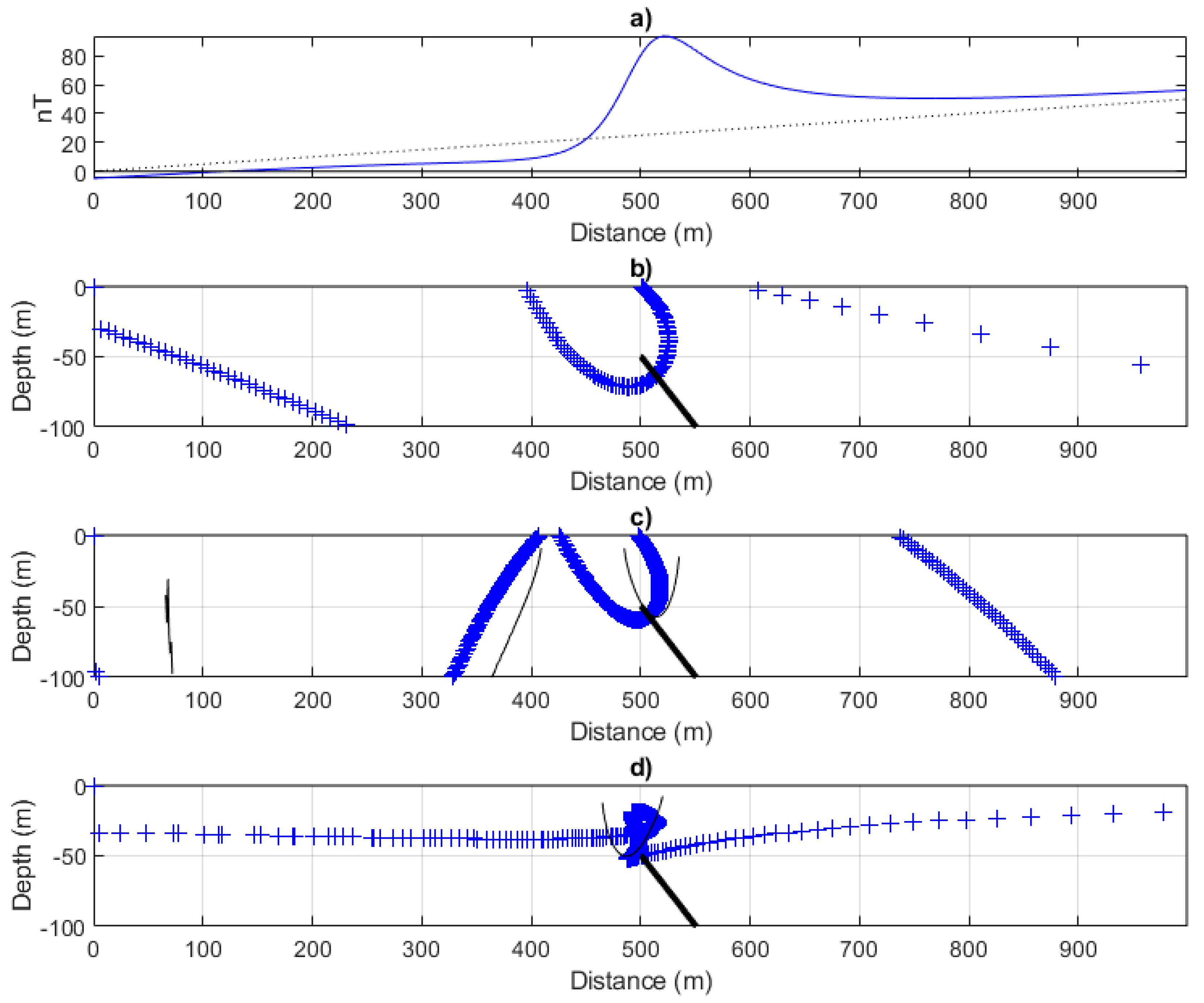
Euler deconvolution is applied to the magnetic anomaly from an isolated dyke (Figure 1), to which a small linear trend has been added. The solutions from standard Euler deconvolution (Equation (2), Figure 1b are widely dispersed around the top of the dyke, while those from the second-order Euler deconvolution (Equations (7) and (10)) are much more tightly grouped (particularly in this case when the Hilbert transform was used). Euler deconvolution is well known for its production of large numbers of spurious solutions scattered throughout the subsurface, and this is the case even with this simple synthetic model. However, plotting the depth parabola provided by Δz = √−a helps to identify the valid solutions, as it should have a maximum depth extent over the source. These depth parabolas are clearly located over the tops of the dykes (Figure 1c,d) and Euler solutions that are far from them can be disregarded.
A second, more complicated example application is shown in Figure 2. In this case, there are now several dykes with different dips and depths, and whose anomalies interfere. All of the methods successfully locate the shallow dyke on the left of the profile. The deeper dykes are more difficult targets, however, and while clusters of solutions are present near them, the clusters are often rather dispersed, and other solutions exist between the dykes. If only the solution clusters that are near to the depth parabolas are considered as being valid, then all the dykes have solutions from the second-order Euler deconvolution lying near to their upper surface (the depth parabola associated with the very shallow dyke is hard to see due to the coincident Euler solutions). Similarly, depth parabolas that are not associated with clusters of Euler solutions can be ignored.
4. Application to a Mineral Exploration Project in Southern Africa
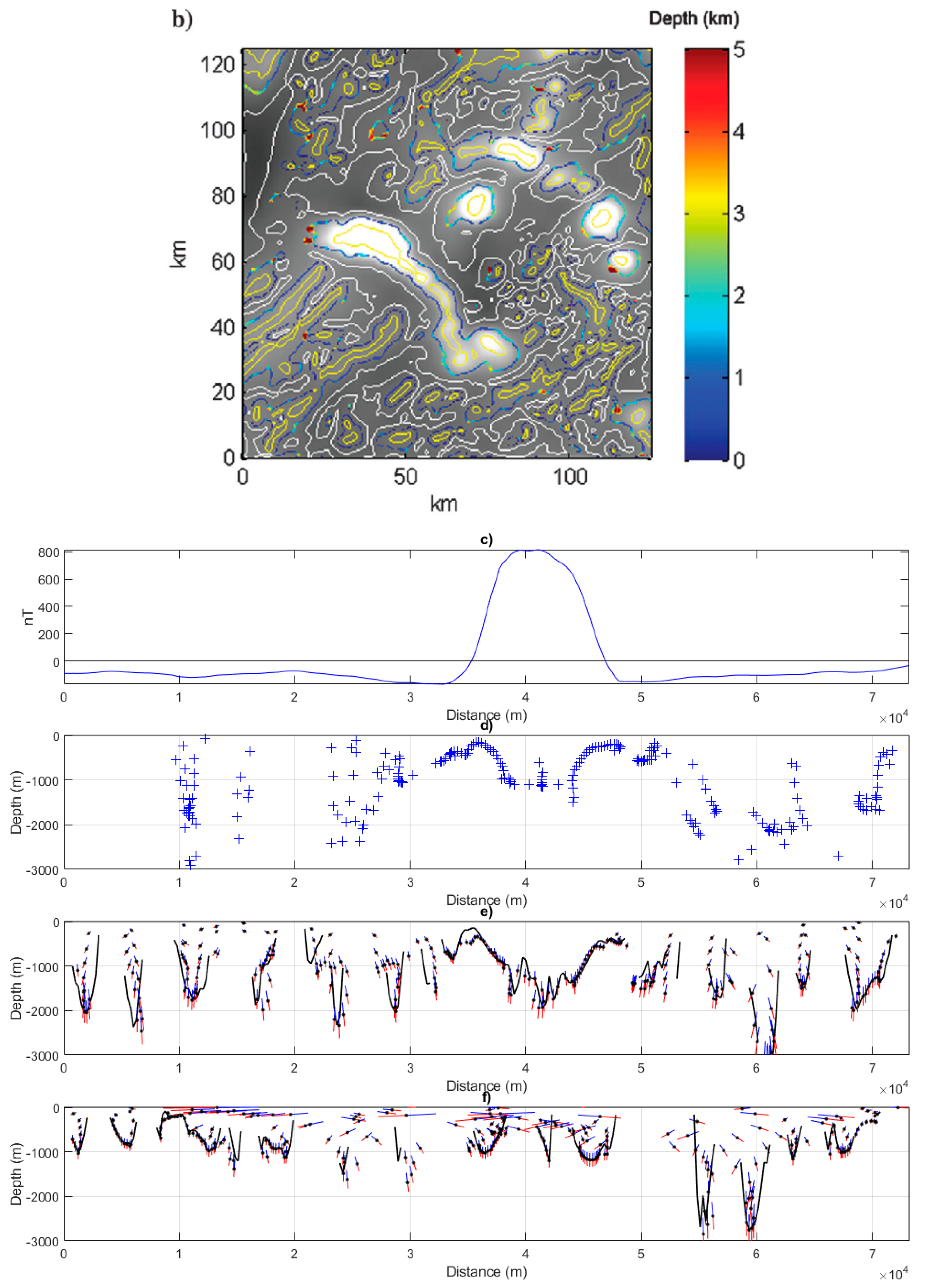
Figure 3a shows an aeromagnetic data set from Southern Africa that was used as part of a mineral exploration project. Unfortunately, confidentiality issues preclude most of the details being provided here. The flight line direction of the survey was north–south, the line spacing was 1 km, the grid interval was 0.25 km, and the flight height was 100 m. This dataset was interpreted by Cooper using a new Contact-Depth method [6], which only works for the magnetic anomalies from contacts and that requires pole reduced data. The depths to the contacts are obtained at the location of the zero values of the first vertical derivative of the data. The results are shown in Figure 3b. Two profiles were abstracted from this aeromagnetic dataset and their locations are marked in Figure 3a. The first profile (marked ‘A’) is shown in Figure 3c, and the results of applying Euler deconvolution to it are shown in Figure 3d–f. The Contact-Depth results provided depths of 1 km or less at the edges of the main anomaly in the centre of the profile, and all the Euler results were compatible with this. The depth parabolas of the second-order Euler method made the interpretation of the Euler solutions easier, particularly those associated from the small amplitude anomalies at the edges of the profile. In addition, varying the structural index slightly allowed the stability of the Euler solutions to be assessed. The red bars associated with each solution show the location that the Euler solutions would move to if a larger SI was used, while the blue bars show the location that will result if the SI were reduced. If these error bars are large (for example, see the shallow solutions in Figure 3f, then those solutions are deemed unreliable.
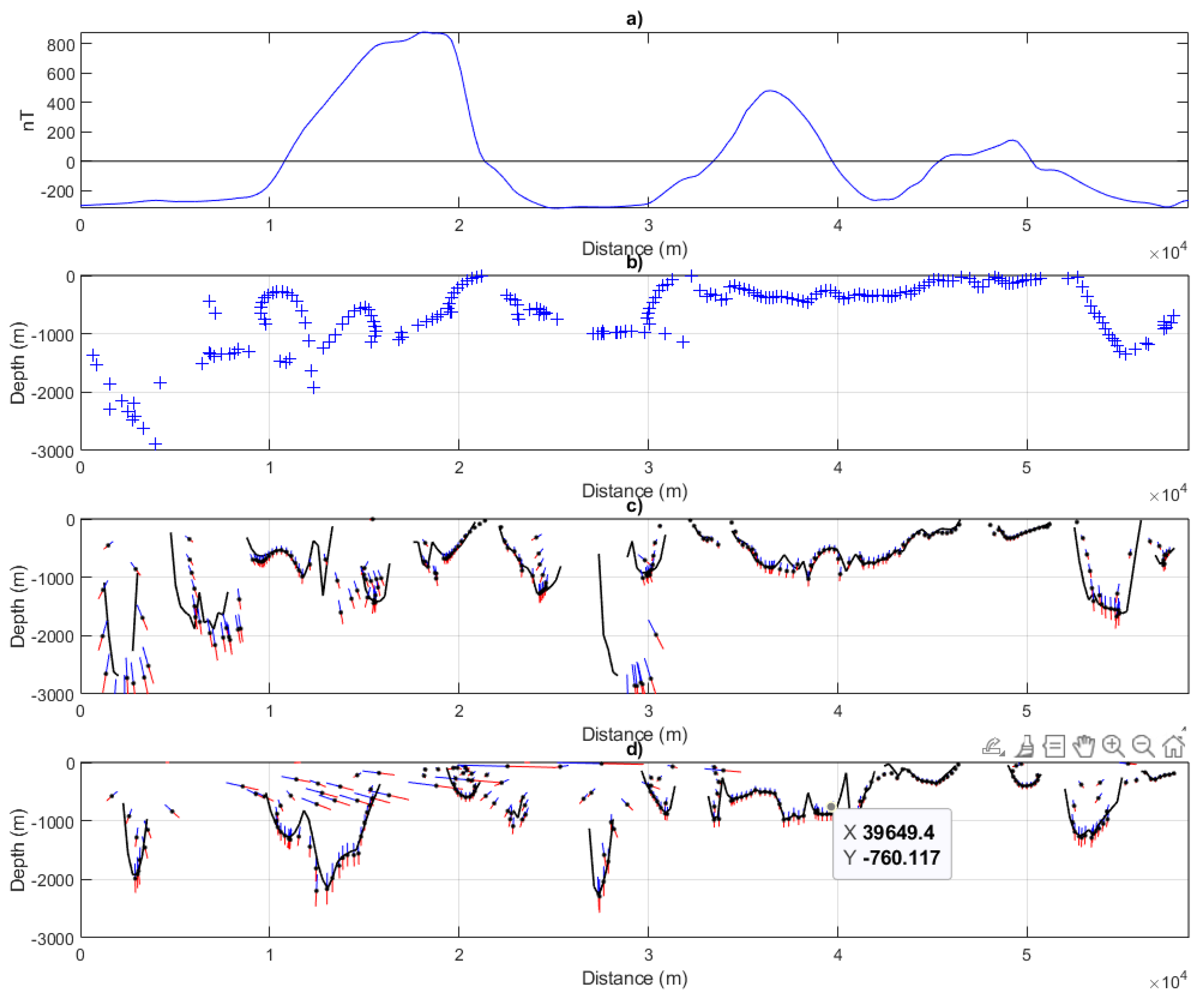
A second profile (marked ‘B’ on Figure 3a is shown in Figure 4. The solutions from standard Euler deconvolution (Equation (2), Figure 4a do not really show well defined clusters, but the depths are reasonable compared with the Contact-Depth results. The solutions from the second-order Euler methods are slightly better clustered, but the depth parabolas help to identify probable solution clusters (e.g., at locations of 15, 25, and 30 km on Figure 4c. The addition of error bars to the plots again helps to identify unreliable solutions, such as the shallow solutions in Figure 4d.
5. Conclusions
Mineral exploration projects have many different facets, and the use of modern data processing techniques can greatly facilitate the process. Second-order Euler deconvolution has been introduced and applied to both synthetic and real aeromagnetic datasets. In addition to being less sensitive to regional trends in the data than standard Euler deconvolution (because it does not use the first order derivatives of the data), it also generates depth parabolas, which further aid in the interpretation of the results. Adding error bars to the Euler solutions shows their sensitivity to the choice of structural index and assists in the assessment of their reliability.
Funding
This research received no external funding.
Data Availability Statement
The data used in this project are confidential and not generally available.
Conflicts of Interest
The authors declare no conflicts of interest.
References
- Fedi, M. DEXP: A fast method to determine the depth and the structural index of potential fields sources. Geophysics 2007, 72, I1–I11. [Google Scholar] [CrossRef]
- Hsu, S.; Sibuet, J.; Shyu, C. High-resolution detection of geologic boundaries from potential-field anomalies: An enhanced analytic signal technique. Geophysics 1996, 61, 373–386. [Google Scholar] [CrossRef]
- Hsu, S.; Coppensz, D.; Shyu, C. Depth to magnetic source using the generalized analytic signal. Geophysics 1998, 63, 1947–1957. [Google Scholar] [CrossRef]
- Keating, P.; Sailhac, P. Use of the analytic signal to identify magnetic anomalies due to kimberlite pipes. Geophysics 2004, 69, 180–190. [Google Scholar] [CrossRef]
- Hartman, R.R.; Teskey, D.J.; Friedberg, J.L. A system for rapid aeromagnetic interpretation. Geophysics 1971, 36, 891–918. [Google Scholar] [CrossRef]
- Cooper, G.R.J. The automatic determination of the location and depth of contacts and dykes from aeromagnetic data. Pure Appl. Geophys. 2014, 171, 2417–2423. [Google Scholar] [CrossRef]
- Cooper, G.R.J. A generalized source-distance semi-automatic interpretation method for potential field data. Geophys. Prospect. 2023, 71, 713–721. [Google Scholar] [CrossRef]
- Huang, L.; Zhang, H.; Sekelani, S.; Wu, Z. An improved Tilt-Euler deconvolution and its application on a Fe-polymetallic deposit. Ore Geol. Rev. 2019, 114, 103114. [Google Scholar] [CrossRef]
- Huang, L.; Zhang, H.L.; Li, C.-F.; Feng, J. Ratio-Euler deconvolution and its applications. Geophys. Prospect. 2022, 70, 1016–1032. [Google Scholar] [CrossRef]
- Reid, A.B.; Allsop, J.M.; Granser, H.; Millett, A.T.; Somerton, I.W. Magnetic interpretation in three dimensions using Euler deconvolution. Geophysics 1990, 55, 80–91. [Google Scholar] [CrossRef]
- Thompson, D.T. Euldph: A new technique for making computer assisted depth estimates from magnetic data. Geophysics 1982, 47, 31–37. [Google Scholar] [CrossRef]
- Mushayandebvu, M.F.; van Drielz, P.; Reid, A.B.; Fairhead, J.D. Magnetic source parameters of two-dimensional structures using extended Euler deconvolution. Geophysics 2001, 66, 814–823. [Google Scholar] [CrossRef]
- Philips, J.D. Two-step processing for 3D magnetic source locations and structural indices using extended Euler or analytic signal methods. In Proceedings of the SEG International Exposition and 72nd Annual Meeting, Salt Lake City, UT, USA, 6–22 October 2002; pp. 1–4. [Google Scholar]
- Cooper, G.R.J. Euler deconvolution applied to potential field gradients. Explor. Geophys. 2004, 35, 165–170. [Google Scholar] [CrossRef]
- Marson, I.; Klingele, E.E. Advantages of using the vertical gradient of gravity for 3-D interpretation. Geophysics 1993, 58, 1588–1595. [Google Scholar] [CrossRef]
- Salem, A.; Ravat, D. A combined analytic signal and Euler method (AN-EUL) for automatic interpretation of magnetic data. Geophysics 2003, 68, 1952–1961. [Google Scholar] [CrossRef]
- Salem, A.; Williams, S.; Fairhead, D.; Smith, R.; Ravat, D. Interpretation of magnetic data using tilt-angle derivatives. Geophysics 2008, 73, L1–L10. [Google Scholar] [CrossRef]
- Pasteka, R.; Richter, F.P.; Karcol, R.; Brazda, K.; Hajach, M. Regularized derivatives of potential fields and their role in semi-automated interpretation methods. Geophys. Prospect. 2009, 57, 507–516. [Google Scholar] [CrossRef]
Figure 1.
(a) Magnetic anomaly from the dyke shown in (b–d) below. A linear trend (dotted line) is added to the data. (b) Solutions from Euler deconvolution (Equation (2)) are shown as blue + symbols. A SI of 1 and window size of 11 points is used. (c) Solutions from second-order Euler deconvolution (Equation (7)) are shown as blue + symbols. A SI of 1 and window size of 11 points is used. The depth parabola is overlain as a black line. (d) Solutions from second-order Euler deconvolution (Equation (10)) are shown as blue + symbols. A SI of 1 and window size of 11 points is used. The depth parabola is overlain as a black line.

Figure 2.
(a) Magnetic anomaly from the dyke model shown in (b-d) below. (b) Solutions from Euler deconvolution (Equation (2)) are shown as blue + symbols. A SI of 1 and window size of 11 points is used. (c) Solutions from second-order Euler deconvolution (Equation (7)) are shown as blue + symbols. A SI of 1 and window size of 11 points is used. The depth parabola is overlain as a black line. (d) Solutions from second-order Euler deconvolution (Equation (10)) are shown as blue + symbols. A SI of 1 and window size of 11 points is used. The depth parabola is overlain as a black line.
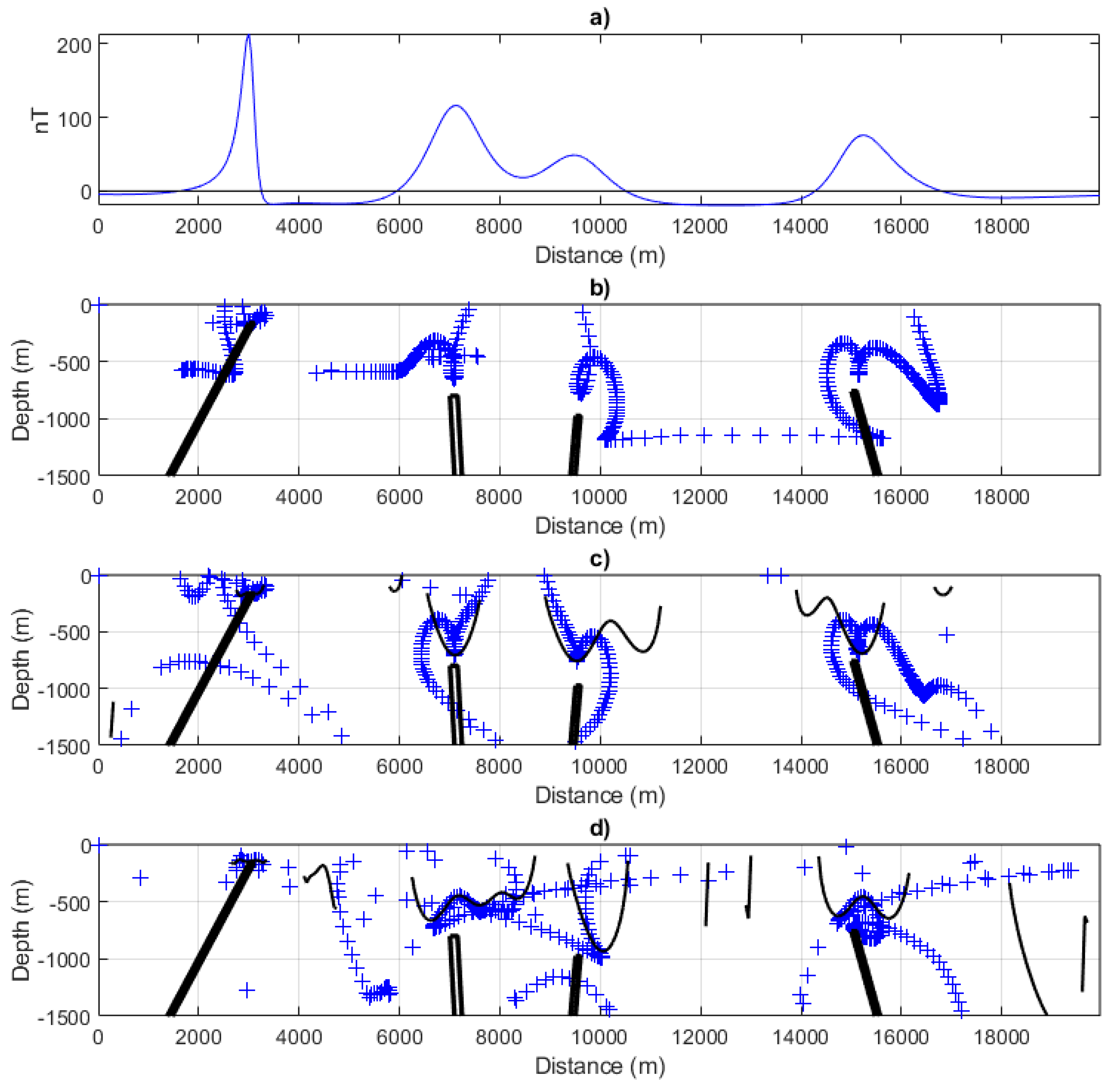
Figure 3.
(a) Aeromagnetic data from Southern Africa. The flight line direction is north–south, the line spacing is 1 km, the grid interval is 0.25 km, and the flight height is 100 m. The profiles marked A (left) and B (right) are shown in Figure 3c and Figure 4a, respectively. (b) Depths to vertically magnetized vertically dipping contacts obtained using the method of Cooper [6], from which the Figure is taken. (c) Aeromagnetic data profile ‘A’ from Figure 3a. (d) Solutions from Euler deconvolution (Equation (2)) are shown as blue + symbols. A SI of 0.25 and window size of 7 points was used. (e) Solutions from second-order Euler deconvolution (Equation (7)) are shown as black dots with blue and red error bars overlain. A SI of 0.25 and window size of 7 points is used. The depth parabola is overlain as a black line. (f) Solutions from second-order Euler deconvolution (Equation (10)) are shown as black dots with blue and red error bars overlain. A SI of 0.25 and window size of 7 points is used. The depth parabola is overlain as a black line.
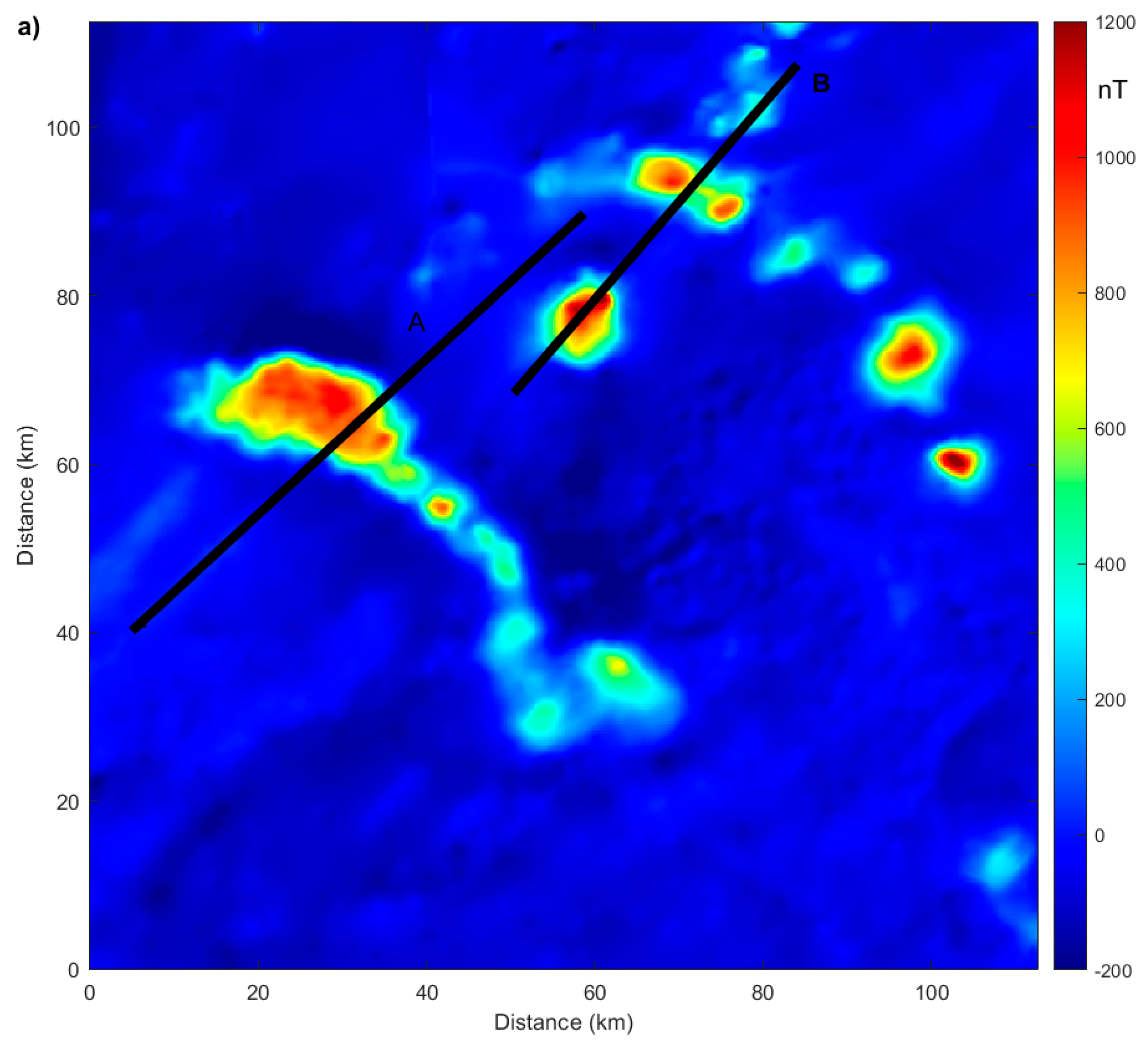

Figure 4.
(a) Aeromagnetic data profile ‘B’ from Figure 3a. (b) Solutions from Euler deconvolution Equation (2)) are shown as blue + symbols. A SI of 0.25 and window size of 7 points is used. (c) Solutions from second-order Euler deconvolution (Equation (7)) are shown as black dots with blue and red error bars overlain. A SI of 0.25 and window size of 7 points is used. The depth parabola is overlain as a black line. (d) Solutions from second-order Euler deconvolution (Equation (10)) are shown as black dots with blue and red error bars overlain. A SI of 0.25 and window size of 7 points is used. The depth parabola is overlain as a black line.

Disclaimer/Publisher’s Note: The statements, opinions and data contained in all publications are solely those of the individual author(s) and contributor(s) and not of MDPI and/or the editor(s). MDPI and/or the editor(s) disclaim responsibility for any injury to people or property resulting from any ideas, methods, instructions or products referred to in the content. |
© 2024 by the author. Licensee MDPI, Basel, Switzerland. This article is an open access article distributed under the terms and conditions of the Creative Commons Attribution (CC BY) license (https://creativecommons.org/licenses/by/4.0/).
Share and Cite
MDPI and ACS Style
Cooper, G.R.J. Using Euler Deconvolution as Part of a Mineral Exploration Project. Minerals 2024, 14, 393. https://doi.org/10.3390/min14040393
AMA Style
Cooper GRJ. Using Euler Deconvolution as Part of a Mineral Exploration Project. Minerals. 2024; 14(4):393. https://doi.org/10.3390/min14040393
Chicago/Turabian StyleCooper, G. R. J. 2024. "Using Euler Deconvolution as Part of a Mineral Exploration Project" Minerals 14, no. 4: 393. https://doi.org/10.3390/min14040393
Note that from the first issue of 2016, this journal uses article numbers instead of page numbers. See further details here.