Potential Toxic Elements Pollution Status in Zones of Technogenic Impact in Central Regions of Perú

Abstract

Soil is a component of the environment. An environmental policy should identify the sources of trace metals in the soil and their effects on people and living beings. The concentrations of 29 surface soil samples (0–25 cm) were determined using the methods EPA 3050B. The data were analyzed using simple and robust statistical analysis that allowed for determining geochemical baseline values. Principal component and correlation analyses were performed, which, together with a spatial analysis, allowed us to distinguish between geogenic and anthropogenic sources. The degree of soil contamination was evaluated using different ecological indices, and the health risks to children and adults were calculated using formulas proposed by the United States Environmental Protection Agency (USEPA). The median concentrations of the analyzed elements correspond to Al 17,666 (mg/kg), As 8.7 (mg/kg), Ba 61.4 (mg/kg), Cd 0.17 (mg/kg), Cr 11.3 (mg/kg), Cu 20.5 (mg/kg), Fe 25,953 (mg/kg), Hg 0.06 (mg/kg), Mn 499 (mg/kg), Ni 20.8 (mg/kg), Pb 15.9 (mg/kg), and Zn 60.6 (mg/kg). In the principal component analysis, four factors were identified that explain 70.3% of the variability of the elements, which, together with the correlation analysis, suggest that the origin of the elements is mainly geogenic with some possible anthropic contributions. The elements analyzed in the soil with moderate contamination correspond to As, Cd, and Pb, in addition, As is the only element that indicated a value above the limit for carcinogenic risk in children. The estimated geochemical baseline values correspond to Al 34,734 (mg/kg), As 15.3 (mg/kg), Ba 113 (mg/kg), Cd 0.41 (mg/kg), Cr 33.8 (mg/kg), Cu 42.9 (mg/kg), Fe 46,181 (mg/kg), Hg 0.12 (mg/kg), Mn 1015 (mg/kg), Ni 42.2 (mg/kg), Pb 21.6 (mg/kg), and Zn 121 (mg/kg). 89.7% of the total samples are at a low level of contamination. The carcinogenic risk due to As in children represents 3.4% of the total samples, so it is considered insignificant.

1. Introduction

Soil contamination is a global problem in which abnormal concentrations of elements or substances that can affect the development of life are generated [1]. Naturally, the content of these elements can have a geogenic origin that can be toxic in high concentrations [2], (although many times this originates from anthropogenic factors. One of the unique properties of soils is their ability to store long-term information about the healthy state of the territory [3].

In Peru, the phenomenon of soil contamination is not an unfamiliar concern. It is a mining and agricultural country with a large number of forest resources, water, and a population of approximately 33,396,700 people [4], that generates solid, organic, or liquid waste that contaminates the water of streams and rivers and, when used in irrigation, increases the concentration of physical and chemical components leading to soil contamination [5]. Moreover, this compartment acts as a sink for a wide variety of emissions as a result of the aerial deposition of particles emitted by human activities comprising several heavy metals, some of which are toxic. In recent years, some researchers have studied the concentrations of heavy metals in the soils of agriculture and mining areas in Peru [6,7,8,9]. The obtained results indicate areas with moderate soil contamination, with elements such as As and Pb being those with the highest concentrations that put people’s health at risk. As a control measure, there is the [10], which was created to regulate the country’s environmental aspects and thus minimize the impact of anthropogenic activities. Peru needs more research on soil contamination to protect human health and ecosystems.

Scientists around the world haven’t agreed on a single method for digestion analysis for an environmental interpretation of PTE concentrations determined in soils. This study used the methods EPA 3050B [11] and EPA 6020B [12]. Changes in environmental components, retrospective and predictive studies of particular systems, as well as regional and global generalizations of the state of the soil system, are becoming increasingly important. Since it is possible to predict changes in the ecological properties of the soil with the incorporation of new human activities in the territory. To identify changes in due time and assess, predict, prevent, and eliminate the consequences of negative processes occurring in the soil with technogenic impact, environmental monitoring of soils is required. In the Central Region of Peru (in the Supplementary Material are included which locations encompass this Region), eight transmission lines with 138 kV, 220 kV, and 500 kV will be constructed and operated within the project “Nueva Yanango-Nueva Huánuco 500 kV link and associated substations”. The transportation sector associated with the construction of transmission lines provides many services. Unfortunately, the adverse effects of transportation have a serious negative impact on the natural environment. It is commonly thought that heavy metals are one of the most important groups among inorganic pollutants related to the transportation sector and infrastructure development [13,14].

The objectives of this study are: (1) to determine the geochemical baseline values of Al, As, Ba, Cd, Cr, Cu, Fe, Hg, Mn, Ni, Pb, and Zn in soils of the Central Regions of Peru; (2) to estimate the level of contamination in soils based on different ecological indices; and (3) to assess the health risk of exposure in children and adults.

2. Materials and Methods

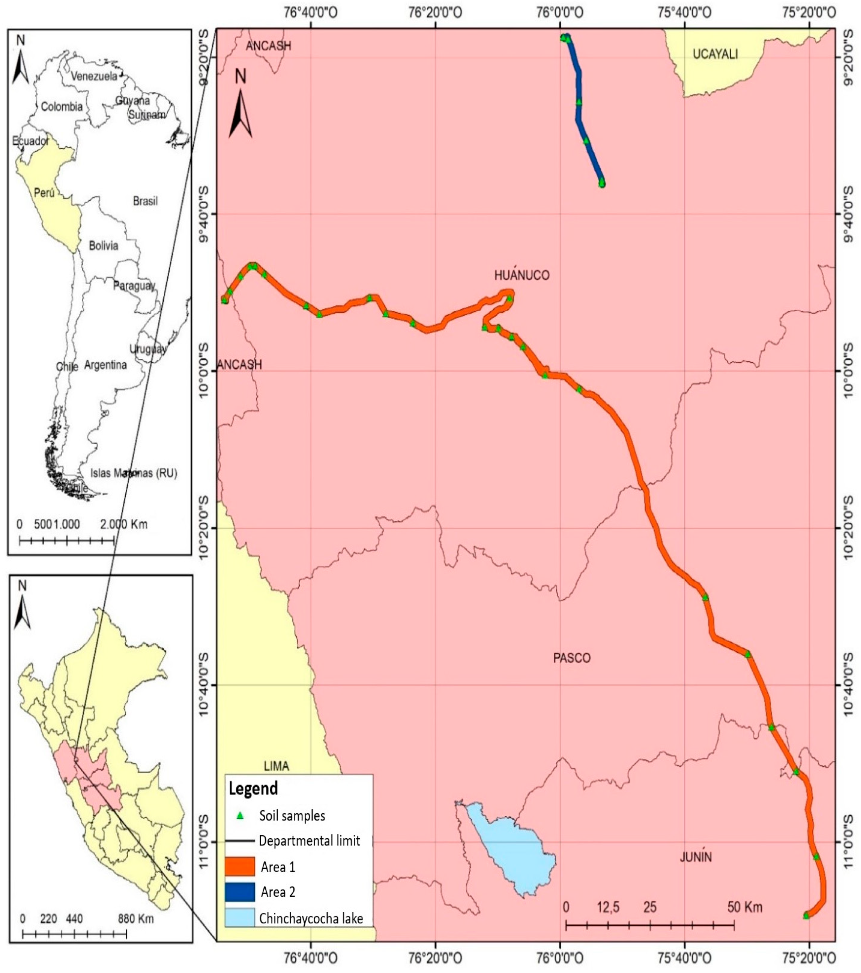
2.1. Study Area

The study zone is located in the Central Regions of Peru, between parallels 9°10′ and 11°40′ south latitude and meridians 74°40′ and 77°20′ west longitude (Figure 1), across the “Nueva Yanango-Nueva Huánuco 500 kV link and associated substations” project. The study zone was divided into two areas, Area 1 and Area 2, linked to transmission lines at 500 kV, and 220 kV–138 kV, respectively. The length of the 500 kV transmission line is approximately 187.46 km, while the associated 220 kV and 138 kV lines total approximately 208 km. The minimum widths of the easement strip considered for the project are 64 m for the 500 kV line, 25 m for the 220 kV line, and 20 m for the 138 kV line [15] , (Figure 1).

The length of the 500 kV transmission line is approximately 187.46 km, while the associated 220 kV and 138 kV lines total approximately 208 km. The minimum widths of the easement strip considered for the project are 64 m for the 500 kV line, 25 m for the 220 kV line, and 20 m for the 138 kV line [15].

The area of direct influence of the study was extended to 50 m on each side of the transmission lines, covering an area of 3788.28 ha where a total of 115 population groups are located (between rural community, village center, housing association, sector, and annex), distributed in the departments of Junín (18), Pasco (6), Huánuco (90), and Ancash (1). The number of inhabitants is estimated at 13,040 [4]. The main economic activities correspond to agriculture and, to a lesser extent, commercial activities. It is important to emphasize that crops include maize (Zea maiz), olluco (Ollucus tuberosus), oca (Oxalis tuberosa), barley (Hurdeum vulgare), wheat (Triticum genus), peas (Pisum sativum), and potatoes (Solanum genus).

Two climatic units were identified. Steppe highlands and puna (highland zone), with a dry and very sunny climate but cold at night, are located in the departments of Ancash and Huánuco. The average monthly temperature varies from 11.1 °C to 23.9 °C and the average monthly precipitation is between 4.6 mm and 88.2 mm, with higher precipitation between December and March. High jungle, with a warm and very humid climate, is located in the departments of Pasco and Junín. The average monthly temperature varies from 5 °C to 22 °C and the average monthly precipitation is between 10 mm and 132 mm, with higher precipitation between December and April. Information was also collected from 12 meteorological stations of the National Meteorological and Hydrological Service of Peru (SENAMHI) close to the study area (with a radius of approximately 50 km) [15].

The geology of the study zone is composed of a series of lithostratigraphic units ranging from the Neoproterozoic to the Cenozoic (Figure 2). Within the area located in the department of Ancash, conglomerates of the La Unión Formation and limestones of the Jumasha Formation and Celedín Formation are identified [16]. Within the department of Huánuco, sequences of shales and gneisses of the Marañón Basal Complex, conglomerate rocks of the Ambo Group, continental rocks of the Mitu Group, carbonate series of the Pucará Group, sandstones and shales of the Sarayaquillo Formation, Goyllarisquizga Group and Oriente Group Formation, limestones of the Chulec-Pariatambo Formation, carbonate deposits of the Chonta Formation, sandstones of the Vivian Formation, limestones of the Jumasha Formation and Celedin Formation, reddish layers of sandstones and clays of the Huayabamba Group and Lantorache Formation, and conglomerates of the La Merced Formation and part of the La Unión Formation [16,17,18,19,20,21]. Lithostratigraphic units such as the Mitu Group, Sarayaquillo Formation, Oriente Group Formation, Chonta Formation (Ks-ch), and Lantorache Formation are also identified within the department of Pasco. The department of Junín includes clastic and carbonate rocks of the Copacabana Group and Chonta Formation and conglomerates of the La Merced Formation [19]. Quaternary deposits such as Morainic Deposits, Fluvioglacial Deposits, Alluvial Deposits (Qr-al), Colluvial Deposits, and Fluvial Deposits are observed in all the departments of the study area [16,17,21]. The study area includes various metallic mineralizations such as Au, Au-Ag, Cu-Pb-Zn-Ag, and Sb-bearing quartz veins found in micaceous shales of the Marañón Complex. Additionally, there are disseminations, veins, and veins of Cu-Ag and Pb-Zn-Ag in sandstones and shales of the Mitu Group. Stratiform bodies of Pb-Zn-Ag are present in limestones of the Pucará Group, and copper deposits in sedimentary rock are found in the Goyllarisquizga Group, as reported by [16].

2.2. Soil Analysis

The concentrations of the elements studied were obtained from the Environmental Impact Study carried out by [15] Consorcio Transmantaro S.A. in 2019 for the “Nueva Yanango-Nueva Huánuco 500 kV Link and Associated Substations” project.

A total of 29 soil samples, 0–25 cm in depth, were obtained contiguous to the vertices of the entire line route. Samples were taken with a plastic shovel and placed in zip-lock bags for transport. The methodology used for sample selection involved environmental criteria such as lithology, life zones, and current land use, as well as technical criteria such as the location of the project components. The samples were obtained to characterize the areas where the main and secondary components of the project will be located and where some contamination could be generated in the future.

The samples were sent to the National Institute of Quality of Peru (INACAL), where the concentrations of metals in soils were determined using the methods EPA 3050B [11] and EPA 6020B [12]. The detection limits for the twelve elements under study were Al 1.09 (mg/kg), As 0.27 (mg/kg), Ba 0.03 (mg/kg), Cd 0.03 (mg/kg), Cr 0.04 (mg/kg), Cu 0.13 (mg/kg), Fe 1.17 (mg/kg), Hg 0.02 (mg/kg), Mn 0.4 (mg/kg), Ni 0.04 (mg/kg), Pb 0.3 (mg/kg), and Zn 0.33 (mg/kg).

2.3. Soil Data Analysis

The results of concentrations obtained from samples below the detection limits were modified by assigning them a value of ½ of the detection limit; duplicate samples were averaged to obtain a single value. Statistical analysis of the data set was performed using RStudio and IBM SPSS Statistics v.21 software (IBM, New York, United Staetes). Histograms, box-plot diagrams, and cumulative frequency plots were obtained for exploratory data analysis (EDA); measures of central tendency, distribution, and dispersion were calculated in univariate statistics; Spearman correlation analysis and principal component analysis (PCA) were used to help identify the origin of pollution sources.

2.4. Spatial Distribution

Spatial distribution was performed using ArcGIS v.10.5 software using ordinary kriging for the twelve elements under study. Figures 8–10 contain the spatial distribution maps generated with ranges divided into 25th, 50th, 75th, 75th, 90th, and 95th percentiles.

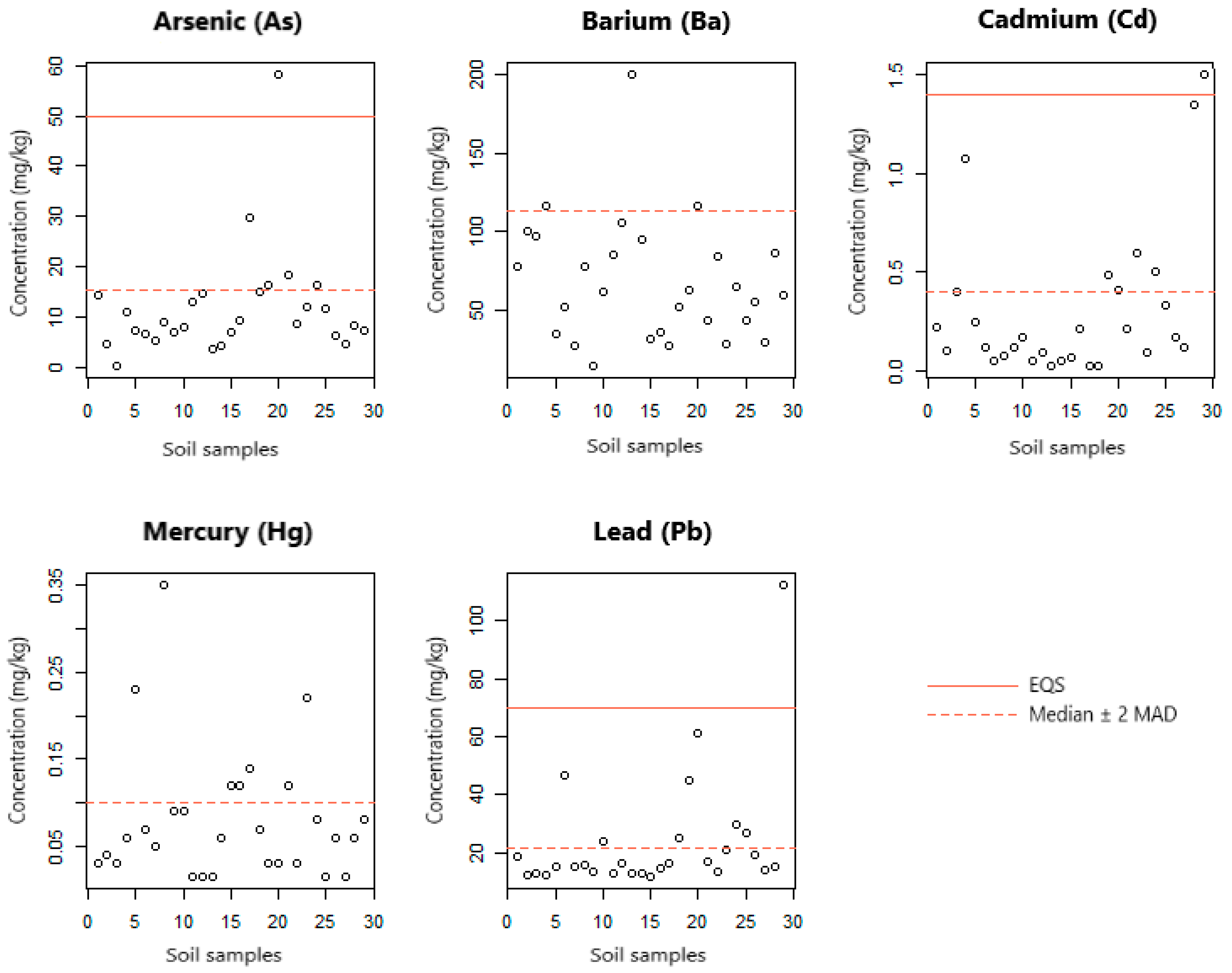
2.5. Threshold Values

The establishment and use of threshold values or geochemical baselines allow the comparison of the estimated value with the actual concentration of the samples and are an important factor in the assessment of possible contamination in soils [22].

At a general level, there are geochemical, or direct, and statistical, or indirect, methods. For this study, the “MAD” method, which uses the median ± 2 absolute deviation from the median [23] the upper whisker method, which is calculated as the 75th percentile + 1.5 interquartile range [24,25]; and the use of the 95th percentile [26,27] were applied and compared. In this study, the MAD method was used for geochemical background values.

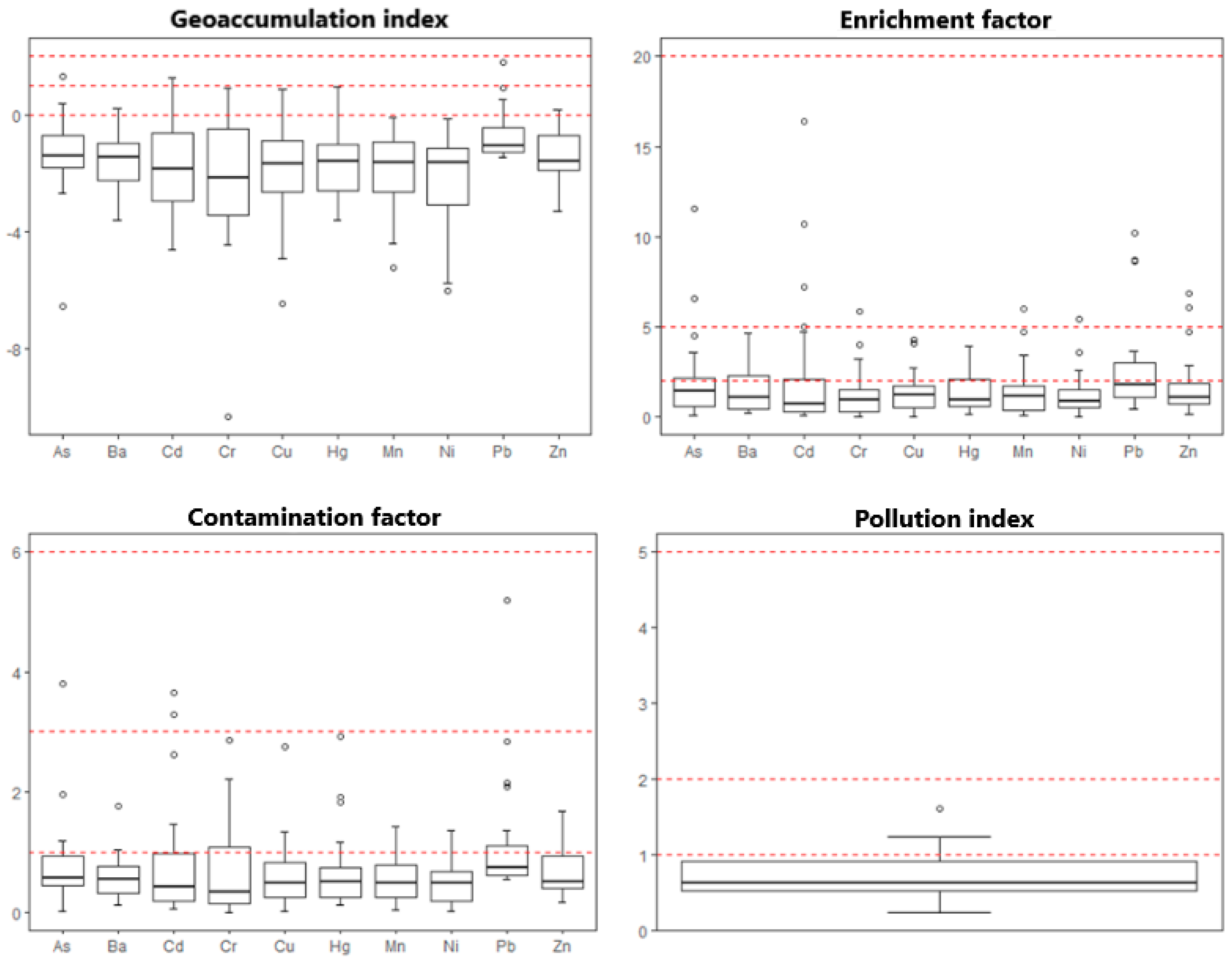
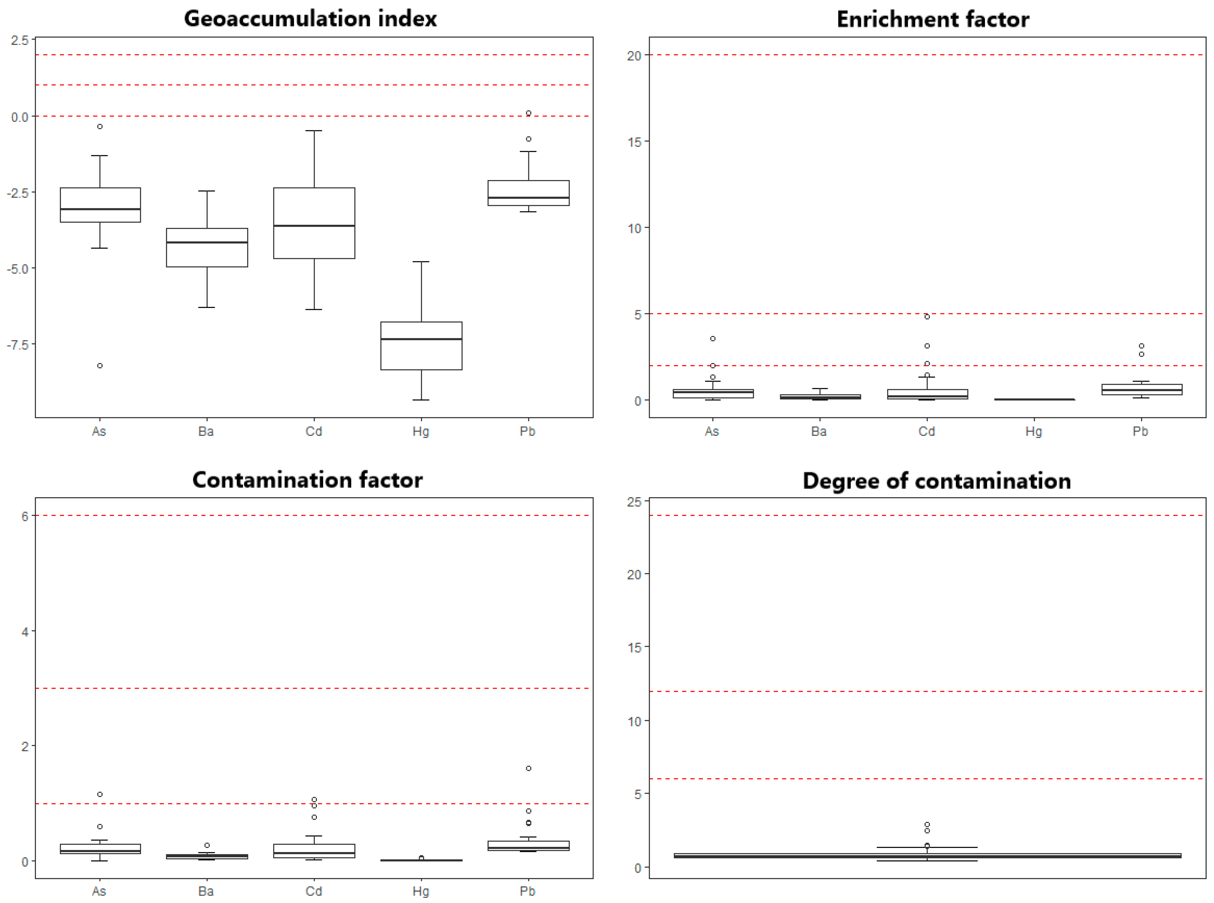
2.6. Environmental Indices

The potential for soil contamination was assessed using several well-established environmental indices [28,29,30]. There are several environmental quality indicators to assess the potential contamination of soils. This study employed several widely used indices to appraise soil contamination: the geoaccumulation index ($I_{GEO}$), enrichment factor ($EF$), contamination factor ($Cf$), pollution index ($IPI$), and degree of contamination ($C_{DEG}$) [25,28,31,32,33].

The geoaccumulation index ($I_{GEO}$) is calculated using Equation (1):

$$I_{GEO}={\log }_2\left(\frac{Cn}{1.5Bn}\right)$$

(1)

where $C_n$ corresponds to the measured content of the element in the soil and $Bn$ is the estimated geochemical baseline value of that element in the soil. The classification according to [29], is shown in Supplementary Material, Table S1 [29,30].

Equation (2) is employed to compute the enrichment factor ($EF$). This metric is established based on the normalization of a tested element against a reference element, with the latter chosen due to its consistently low occurrence variability. As suggested by [34] Sc, Mn, Ti, Al, and Fe are frequently employed as reference elements. In this particular investigation, Al serves as the reference element for eleven of the twelve analyzed elements, and Fe acts as the reference element for standardizing Al. Their minimal variability influences the choice of these elements in the soils traversed by the transmission line for this study.

$$EF=\frac{\frac{C_i}{C_{ref}}}{\frac{C_{oi}}{C_{oref}}}$$

(2)

where $C_i$ is the concentration of the element in the sample, $C_{oi}$ is the corresponding geochemical baseline value, $C_{ref}$ is the concentration of the reference element in the sample, and $C_{oref}$ is the geochemical baseline value of that element (in mg/kg). Table S6 shows the classification of EF [30].

The contamination factor is calculated using Equation (3):

$$Cf=\frac{C_i}{C_{oi}}$$

(3)

where $C_i$ is the concentration of the element in the sample and $C_{oi}$ is the corresponding geochemical baseline value. Table S7 shows the classification of the contamination factor [28].

The pollution index is defined as the average of the pollution factors calculated for each of the elements. Its calculation method is presented in Equation (4):

$$IPI={\displaystyle \sum \frac{Cf}{n}}$$

(4)

The classification of $IPI$ values is shown in Table S1.

The last method corresponds to the contamination degree ($C_{DEG}$), defined as the sum of the individual contamination factors. Its calculation method is presented in Equation (5):

$$C_{DEG}={\displaystyle \sum Cf}$$

(5)

The classification for the contamination degree proposed by [28] was based on eight elements. In this study, the $C_{DEG}$ was used in the evaluation of the five pollutants with EQS values for agricultural soils, so a modification was made according to that proposed by [32]). Table S8 shows the classification of the contamination factor.

2.7. Environmental Indices with Peruvian Environmental Quality Standards (EQS) for Soil

Additionally, for comparison purposes, the concentrations of potentially toxic elements were compared against the maximum permissible limits established by Peruvian legislation in Supreme Decree N° 011-2017-MINAM [35] for agricultural soils.

The EQS values are presented in Table S2 and are established for some elements.

2.8. Health Risks

Carcinogenic and non-carcinogenic health risks were evaluated using formulas derived by the US Environmental Protection Agency [36,37,38,39].

High concentrations of potentially toxic elements (PTEs) in soils pose various health risks to humans. To evaluate these risks, the United States Environmental Protection Agency (USEPA) has established reference doses (RfDs) that allow for the assessment of carcinogenic and non-carcinogenic risks associated with ingestion, dermal absorption, and inhalation as exposure pathways [36,39,40]. The daily doses received through ingestion (ADI_ing), dermal absorption (ADI_dermal), and inhalation (ADI_inh) were calculated using Equations (6)–(8), adapted from various USEPA publications [36,38,39,40].

$$AD{I}_{ing}=C_{soil}\times \left(\frac{IngR\times EF\times ED}{BW\times AT}\right)\times {10}^{-6}$$

(6)

$$AD{I}_{dermal}=C_{soil}\times \left(\frac{SA\times AF\times ABS\times ED}{BW\times AT}\right)\times {10}^{-6}$$

(7)

$$AD{I}_{inh}=C_{soil}\times \left(\frac{InhR\times EF\times ED}{PEF\times BW\times AT}\right)\times {10}^{-6}$$

(8)

where the total element concentration in soil is denoted by $C_{soil}$ (mg/kg), the intake rate by $IR$ (mg/day), the exposure frequency by $EF$ (days/year), the exposure duration by (years), body weight by $ED$ (kg), and the average exposure time by $AT$ (days), calculated as AT = ED × 365. The surface area is represented by $SA$ (cm²), the skin adhesion factor by $AF$ (mg/cm²), the dermal absorption factor by $ABS$ (dimensionless), the inhalation rate by $InhR$ (m³/day), and the particulate emission factor by $PEF$ (m³/kg). The values of these parameters used in the study are presented in Table S3.

2.8.1. Non-Carcinogenic Risk

For the non-carcinogenic risks, Equations (9)–(11) show how the hazard quotient (HQ) is derived for each exposure route. To further evaluate the overall potential for non-carcinogenic effects by all exposure routes and to estimate the combination risks, Equation (12) is used, which gives the hazard index ($HI$).

$$H{Q}_{ing}=\frac{AD{I}_{ng}}{Rf{D}_o}$$

(9)

$$H{Q}_{dermal}=\frac{AD{I}_{dermal}}{Rf{D}_d}$$

(10)

$$H{Q}_{inh}=\frac{AD{I}_{inh}}{RF{D}_i}$$

(11)

$$HI=H{Q}_{ing}+H{Q}_{dermal}+H{Q}_{inh}$$

(12)

where $RF{D}_o$ corresponds to the oral reference dose (soil ingestion), $RF{D}_d$, the dermal soil absorption reference dose, and $RF{D}_i$ the inhalation reference dose of soil particles (mg/kg/day).

The values used for this study are presented in Table S4 and were compiled from USEPA [38,41,42,43]. $HI$ values > 1 expose a significant risk to human health [33,44].

2.8.2. Carcinogenic Risk

The carcinogenic risk is based on the values for ingestion ($AD{I}_{ng}$), dermal absorption ($AD{I}_{dermal}$), and inhalation ($AD{I}_{inh}$) calculated by Equations (9)–(11), using the time over which the dose for carcinogens (AT-C) is averaged. For each route of intake, the carcinogenic risk ($CR$) is calculated through Equations (13)–(17), and finally, the cumulative or total carcinogenic risk ($TCRI$) is calculated using Equation (18). It should be noted that for this study, the oral carcinogenic risk was assessed only for As, Pb, Cr, and Ni because they were the only available $S{F}_o$ values [40].

$$C{R}_{ing}=AD{I}_{ing}\times S{F}_o$$

(13)

$S{F}_o$ the oral slope factor (mg/kg/día)⁻¹

$$C{R}_{dermal}=AD{I}_{dermal}\times S{F}_d$$

(14)

$S{F}_d$ is the dermal slope factor (mg/kg/day)⁻¹ obtained by Equation (15).

$$S{F}_d=\frac{S{F}_o}{AB{S}_{Gi}}$$

(15)

where $AB{S}_{Gi}$ corresponds to gastrointestinal absorption without units.

$$C{R}_{inh}=AD{I}_{inh}\times S{F}_i$$

(16)

$S{F}_i$ is the inhalation slope factor (mg/kg/day)⁻¹ obtained by Equation (17).

$$S{F}_i=URF\times \frac{1}{InhR}\times BW\times {10}^3$$

(17)

$URF$ is the unit of risk factors (m³/μg); $InhR$ is the inhalation rate (m³/day); BW is body weight (kg); and 10³ is the unit conversion factor.

$$TCRI={\displaystyle \sum \left(AD{I}_{ing}\times S{F}_o\right)}+{\displaystyle \sum \left(AD{I}_{dermal}\times S{F}_d\right)}+{\displaystyle \sum \left(AD{I}_{inh}\times S{F}_i\right)}$$

(18)

$TCRI$ values > 10⁻⁴ indicate a significant carcinogenic risk to human health, while $TCRI$ < 10⁻⁶ indicate that exposure is not harmful [37]. Table S5 shows the URF values obtained from [45].

3. Results and Discussion

3.1. Exploratory Data Analysis

Figures S1–S3 present the different histograms, box-plot diagrams, and cumulative frequency plots obtained, which allow summarizing the main characteristics of the data under study. The histograms obtained show that the elements follow an asymmetric distribution of positive biases to the right. Elements such as As, Cr, Cu, Hg, and Pb are those that fit best as described. Some isolated bars are also observed that represent data values far away from the other data values, called outliers. The latter can be best observed for the elements As, Ba, Cd, Fe, Hg, and Pb in the box-plot diagrams, where these outliers are represented as points outside the upper whisker. Based on the cumulative frequency plots, it can be seen that none of them adopt a 45° straight line, i.e., it reaffirms the description that no element adopts a normal distribution.

3.2. Univariate Statistics

Table 1. Statistical summary of the concentrations of potentially harmful elements (mg/kg) in soil samples from the project.

PTE	Mean	S.D.	C.V%	Bias	Kurt.	Min	P25	P50	P75	Max	MAD
Al	20,053	11,301	56.4	0.82	0.14	6634	10,855	17,666	26,934	47,919	8534
As	11.7	10.7	91.4	2.9	13.1	0.25	6.6	8.7	14.3	58.1	3.3
Ba	67.6	38.7	57.3	1.3	3.5	14.2	35.8	61.4	86.1	200	25.7
Cd	0.31	0.38	125	1.9	4	0.03	0.08	0.17	0.4	1.5	0.12
Cr	22.5	25.4	113	1.3	1.5	0.04	4.8	11.3	36.9	96.9	11.3
Cu	25.5	23.4	91.8	2.1	7.9	0.74	10.5	20.5	35.1	118	11.2
Fe	30,301	19,128	63.1	1.3	1.9	5164	19,012	25,953	36,592	82,787	10,114
Hg	0.08	0.08	94.3	1.9	5	0.01	0.03	0.06	0.09	0.35	0.03
Mn	578	411	71.1	0.52	−0.57	41.4	246	499	799	1446	258
Ni	22.3	17	76.1	0.66	−0.25	0.97	7.5	20.8	28.5	57.7	10.7
Pb	23.6	20.7	87.5	2.9	12.1	11.8	13.5	15.9	24.1	112	2.9
Zn	79.2	45.9	58	0.81	0.19	18.7	48.5	60.6	112	204	30.1

PTE potentially toxic element, S.D. standard deviation, CV% coefficient of variation (%), Kurt. Kurtosis, Min minimum, P25 25th percentile, P50 50th percentile, P75 75th percentile, Max maximum, ADM absolute deviation from the median.

presents the summary statistics for the elements under study. The elements with the highest mean concentration values are Al and Fe, which is because they are major elements in the soils [46]. The coefficients of variation are higher than 80% for elements such as As, Cd, Cr, Cu, Hg, and Pb, so their mean is not representative of the set. In addition, large differences between minimum and maximum values are observed, indicating heterogeneity in the data.

Table 2. Median concentrations of potentially toxic elements (mg/kg) reported in publications on agricultural soils in Peru.

PTE	La Zanja	Colquirrumi	Julcani	La Pastora	Comunidad de Infierno	This Study
Al	-	-	-	-	-	17,666
As	15.2	477	24.4	6.4	3.7	8.7
Ba	-	-	-	-	-	61.4
Cd	2.3	17.8	6	0.8	<0.02	0.17
Cr	5.2	14.4	16.4	-	-	11.3
Cu	12.5	222	9.4	2.2	0.63	20.5
Fe	-	-	-	85	48.3	25,953
Hg	0.15	4	4.6	-	-	0.06
Mn	-	-	-	6.4	14.1	499
Ni	57.3	18.3	11.1	-	-	20.8
Pb	35	1296	238.4	11	7.2	15.9
Zn	44	2651	90.4	0.99	1.3	60.6
Sample	21	20	18	12	12	29
Reference	[8]	[8]	[8]	[9]	[9]	This study

contains a summary of the median concentrations (mg/kg) reported in some publications on Peruvian soils. A comparison with the data obtained in this study shows that the concentrations of As, Cd, Hg, and Pb are higher in the Colquirrumi, Julcani, and La Zanja sectors, which may be since, although these were natural areas with land use considered agricultural, they correspond to areas with a high density of mining sites in operation.

On the other hand, the Infierno Community, which is a control site with agricultural land use that has not been impacted by mining activity and there are no records of this activity in the vicinity, reports the lowest concentrations of most of the elements under study. In the area of La Pastora, the concentrations are similar to the previously described sector, with some variations since they correspond to agricultural land use in an area abandoned by gold mining exploitation.

3.3. Multivariate Statistics

Since the data do not follow a normal distribution, Spearman’s method was used for the correlation matrix between the twelve elements under study, all samples (

Table 3. Spearman correlation matrix between concentrations of potentially harmful elements (mg/kg) in soil samples from the project.

	Al	As	Ba	Cd	Cr	Cu	Fe	Hg	Mn	Ni	Pb	Zn
Al	1	−0.17	−0.35	−0.29	0.34	−0.12	0.31	0.29	−0.21	0.04	0.01	−0.13
As		1	−0.04	0.17	0.25	0.33	0.22	0.12	0.32	0.18	0.5 **	0.31
Ba			1	0.22	1 × 10−3	0.33	−0.07	−0.52 **	0.43 *	0.38 *	−0.17	0.47 *
Cd				1	−0.2	−0.08	−0.37 *	−0.07	0.4 *	0.12	0.3	0.5 **
Cr					1	0.62 **	0.77 **	−0.03	0.13	0.72 **	−0.08	0.23
Cu						1	0.74 **	−0.06	0.44 *	0.68 **	0.09	0.42 *
Fe							1	−0.04	0.17	0.56 **	0.07	0.16
Hg								1	−0.13	−0.25	0.11	−0.36
Mn									1	0.35	0.28	0.46 *
Ni										1	−0.14	0.54 **
Pb											1	0.37 *
Zn												1

(*) Correlation is significant at the 0.05 level; (**) Correlation is significant at the 0.01 level.

). The elements with the best correlation, ordered from highest to lowest, are Fe-Cr, Fe-Cu, Ni-Cr, Cu-Ni, Cu-Cr, Fe-Ni, Zn-Ni, and Pb-As. According to [47], in the Huánuco Region, the metamorphic and ultramafic rocks of the Marañon Basal Complex have a high content of magnetite and mineralization of Fe, Ni, and Cu, so the high correlations between these elements could be due to their common geogenic origin. Regarding correlations such as Pb-As, they may be generated because inorganic arsenic occurs naturally in the soil and many types of rocks, especially in ores containing copper or lead [48].

Table 4. Factor analysis matrix for soil samples from the project.

Element	Component
	1	2	3	4
Al	−0.12	0.61	−0.03	0.48
As	0.27	−0.15	0.62	−0.45
Ba	0.45	−0.3	−0.45	−0.42
Cd	0.55	−0.55	0.05	0.43
Cr	0.61	0.62	−0.17	0.16
Cu	0.61	0.57	0.09	−0.25
Fe	0.47	0.73	0.12	−0.2
Hg	−0.27	0.37	0.51	0.27
Mn	0.53	−0.14	0.4	−0.24
Ni	0.78	0.11	−0.33	0.21
Pb	0.46	−0.34	0.45	0.42
Zn	0.75	−0.37	−0.05	0.17
Variance %	27.4	20.5	11.5	10.8
Cumulative Variance%	27.4	47.9	59.4	70.3

presents the factor analysis matrix obtained through principal component analysis of all samples. The number of components was reduced to four based on the sedimentation plot and the Kaiser criterion, which indicates using principal components with eigenvalues greater than one [49]. Additionally, items with absolute loading values equal to and/or greater than 0.45 were considered to describe the principal composition of each factor.

The four principal components explain 70.3% of the total variance of the data. Component 1 explains 27.4% of the total variance, with the associated elements being Ni, Zn, Cr, Cu, Cd, Fe, Pb, and Ba. These elements are usually related to the parent material, so this component may be related to a natural factor such as the lithology and geology of the existing rock. Component 2 explains 20.5% of the total variance, with the associated elements being Fe, Cr, Al, Cu, and the negative sign Cd. It is possible to observe in the cluster analysis (Figure 2) how Fe and Al are grouped in the third level, while Cr and Cu are in the first level. Component 3 explains 11.5% of the variance, with As and Hg being associated as well as Ba and Pb with equal but opposite loadings. Finally, component 4, which explains 10.8% of the variance, has the elements Al and As associated with similar charges, with opposite signs. Most of the elements contain high values in more than two components, which would indicate that their source may be more than one. For the cluster analysis, two dendrograms were generated using Ward’s method and Euclidean distance, the first one considering the twelve elements under study, while the second one did not consider Al and Fe because they are considered major elements, allowing the different groups generated to be appreciated on a larger scale (Figure 3).

The first level shows most of the elements under study, which have formed three groups very close to each other composed of Ba-Zn, As-Cd-Hg, and Pb-Cu-Cr-Ni. The second level shows Mn, which has a significant charge level only for the first main component, together with elements such as Cu, Cr, Ni, and Zn. Finally, a third level is observed with the group composed of Al and Fe, which could have been differentiated from the other elements due to their high concentrations. Elements such as Cd, Cr, Cu, and Pb suggest more than one source of origin. Cd is strongly associated with Zn, Cu, and Pb minerals, but since a number of the samples were obtained from agricultural soils, phosphate fertilizers, and sewage sludge, could be contributing to the increase in Cd levels [50]. Similarly, although the samples are located at distances of at least 30 m from roads and secondary roads, there is a possibility that the Pb concentrations located in the South of Area 2 could be influenced by vehicular traffic [51].

3.4. Threshold Values and Assessment of Potential Contamination

Table 5. Threshold values (mg/kg) with three calculated methods (median ± 2 MAD, TIF upper whisker method, and P95 95th percentile) and outliers’ number of samples with concentrations above the geochemical baseline value in surface soil samples (0–25 cm) from the project.

	Al	As	Ba	Cd	Cr	Cu	Fe	Hg	Mn	Ni	Pb	Zn
Median ± 2 MAD	34,734	15.3	113	0.41	33.8	42.9	46,181	0.12	1015	42.2	21.6	121
Outliers	3	5	3	6	8	4	4	4	6	5	8	7
Percentage	10.3%	17.2%	10.3%	20.7%	27.6%	13.8%	13.8%	13.8%	20.7%	17.2%	27.6%	24.1%
TIF	51,053	25.8	162	0.9	85.0	71.8	62,963	0.18	1629	60.1	40.0	207
Outliers		2	1	3	1	1	3	3			4
Percentage		6.9%	3.4%	10.3%	3.4%	3.4%	10.3%	10.3%			13.8%
P95	42,090	25.3	116	1.2	70.0	56.3	74,014	0.23	1302	55.7	55.4	142
Outliers	2	2	2	2	2	2	2	2	2	2	2	2
Percentaje	6.9%	6.9%	6.9%	6.9%	6.9%	6.9%	6.9%	6.9%	6.9%	6.9%	6.9%	6.9%

presents the threshold values obtained by the different methods described in Section 2.4. The upper limits of the geochemical baseline content differ mainly between the TIF and the P95 concerning the median ± 2 MAD. The median ± 2 MAD is better at reducing the geochemical baseline upper limit than the other two. The highest upper limits are obtained with TIF except for Cd, Fe, Hg, and Pb, which are obtained with P95. The soils have been predominantly influenced by natural element dispersion and accumulation processes, but there are a few points with an anthropic influence. Cd and Pb are the heavy metals with the highest number of outliers in the three methods. Regarding the baseline values established by [48] in soils of the Andes Mountain Range (Peru), the upper limit of the geochemical baseline of this study is higher in Cr, Cu, Zn, and Pb, while the values established for As, Cd, and Hg are lower for the three methods studied. The most plausible calculation of the geochemical baseline in the soils of the Central Regions of Perú was tested using the median ± 2 MAD. Therefore, the ranges obtained by the calculated distribution are chosen as geochemical baseline values.

3.5. Assessment of Potential Contamination

The Environmental Quality Standards (EQS) for soil were evaluated considering that the majority of the extracted samples were collected from non-intervention and agricultural areas. Figure 4 presents a graphical representation of the results for all samples.

Sampling point 20 showed an As concentration of 58.1 mg/kg, exceeding the EQS for agricultural land use. This point is located in the Huánuco department, northwest of study Area 1, on a Jumasha geological formation with a predominantly limestone lithology. The current land use is crop cultivation, and it is situated 23.9 m from the project’s closest vertex. The elevated As value is hypothesized to be of geogenic origin or due to the area’s mineralogy, which could have been influenced by fertilizer application. Sampling point 29 presented Cd and Pb concentrations of 1.5 mg/kg and 112.1 mg/kg, respectively, both exceeding the EQS for agricultural land use. This sampling point is located in the Huánuco department, southeast of study area 2, on a Pucará geological group with a predominant lithology of limestone. The current land use is grassland in a secondary forest. The elevated Cd and Pb values are suggested to be of geogenic origin or due to the metallic mineralization in the limestones, a characteristic of the present geological unit.

The reason for the deviation caused by normalizing the results with different threshold values is that EQS values are higher than the MAD method. The EQS values are generic reference values (GRL) or soil screening values (SSV). Generic reference values are typically established by assessing the potential harm they can cause to receptors such as humans or ecosystems. This evaluation considers both the contaminant’s inherent toxicity and the level of exposure experienced by the receptors at risk [52].

Table S6 summarizes the results obtained for the geoaccumulation index ($I_{GEO}$), enrichment factor ($EF$), contamination factor ($Cf$), and pollution index ($IPI$) for ten of the elements under study. The geochemical baseline values used in the assessment are those provided by the median ± 2 MAD method, as it provides the highest number of outliers. These results are visually represented through box-plot diagrams in Figure 5.

According to the values obtained for the geoaccumulation index, the elements analyzed are in the uncontaminated to moderately contaminated range. Cd, As, and Pb are those elements with samples within the latter range, but only representing 6.9% and 3.4% of the total analyzed samples.

For the ($EF$), the elements analyzed fall between the poorly to significantly enriched ranges. Elements within the latter range only represent between 3.4% and 10.3% of the total of the analyzed samples. Regarding the contamination factor, between 3.4% and 6.9% of the total samples analyzed for Cd, As, and Pb are categorized as significantly contaminated. For the pollution index, 89.7% of the total samples are at a low level of contamination.

The geoaccumulation index ($I_{GEO}$), enrichment factor ($EF$), contamination factor ($Cf$), and degree of contamination ($C_{DEG}$) were also evaluated using the ($EQS$) values for agricultural land use as geochemical baseline values. The results are presented graphically in Figure 6.

The values obtained for the geoaccumulation index indicate that only one value for Pb is in the moderately contaminated range. 100% of the samples for As, Ba, Cd, and Hg are in the practically uncontaminated range. The analyzed elements are in the low to moderate enrichment range. The elements As, Cd, and Pb in the latter range represent only between 6.9% and 10.3% of the total analyzed samples. This indicates that 3.4% of the total analyzed samples for As, Cd, and Pb are within the moderate contamination range. Finally, the $C_{DEG}$ indicates that 100% of the total samples are in the low contamination range.

3.6. Health Risks

For the non-carcinogenic risks, Table S7 presents a summary of the results obtained. It is observed that for the non-carcinogenic risk in children, the elements As, Mn, Cr, and Pb contain at least 20.7% of the samples above the significant risk limit, with As and Mn representing high risks for 96.6% and 79.3% of the total samples. For the non-cancer risk in adults, only As contains samples outside the safe limit, representing 10.3% of the total number of samples. For carcinogenic risks in children, only As shows values above the limit, although these represent only 3.4% of the total samples. For carcinogenic risks in adults, As is within the acceptable risk range (S8). The results obtained can also be observed graphically through the box-plot diagrams in Figure 7.

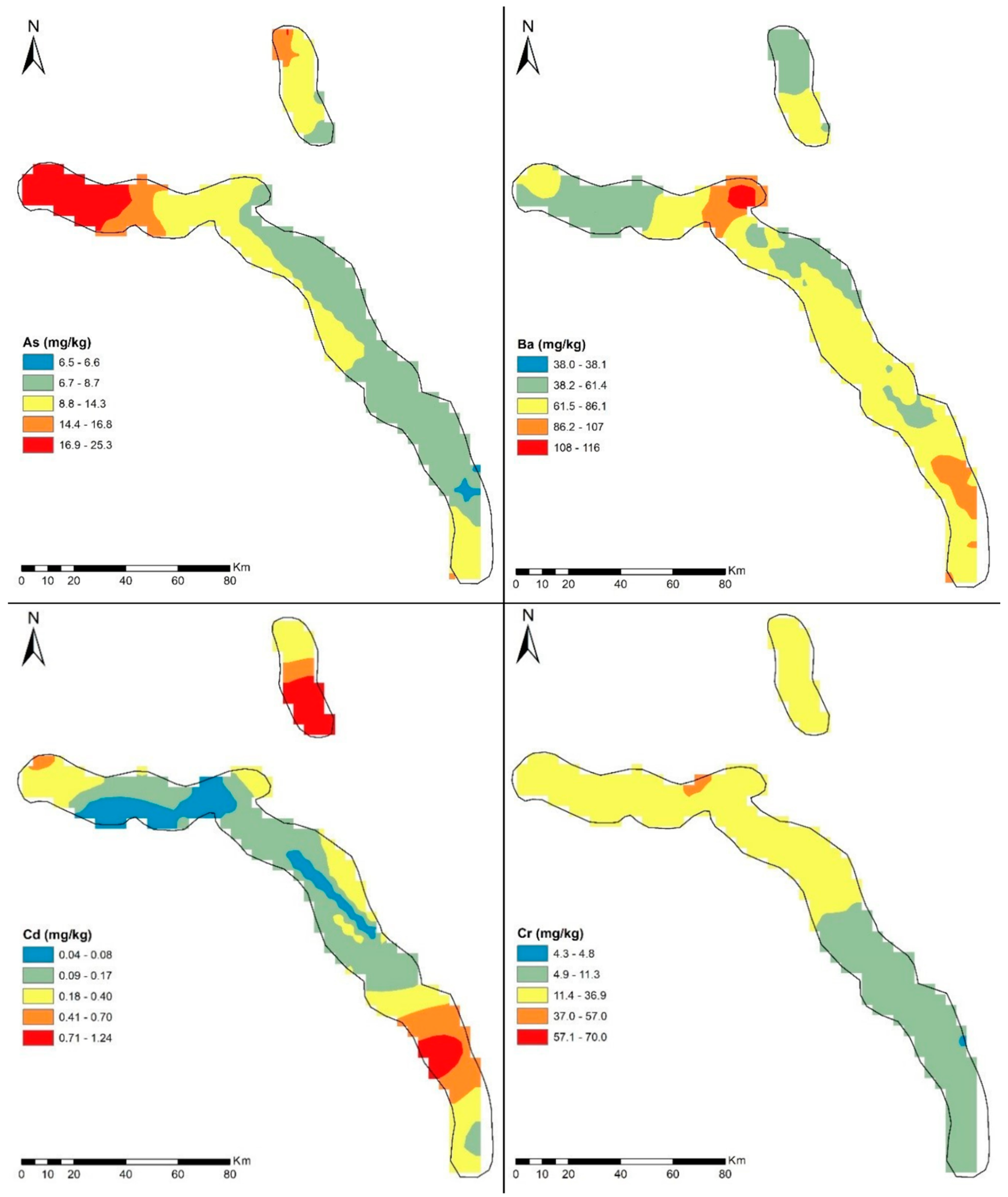
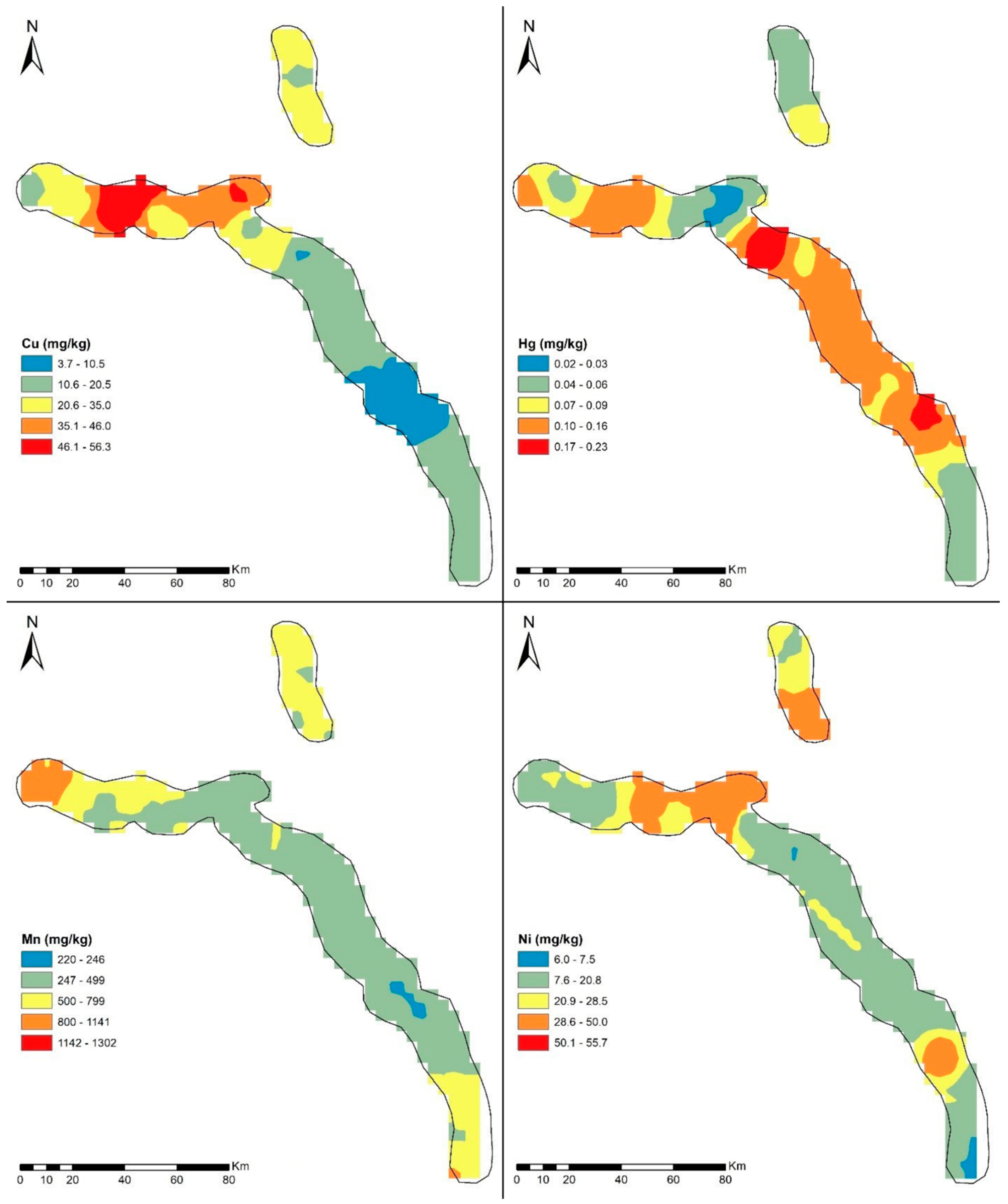
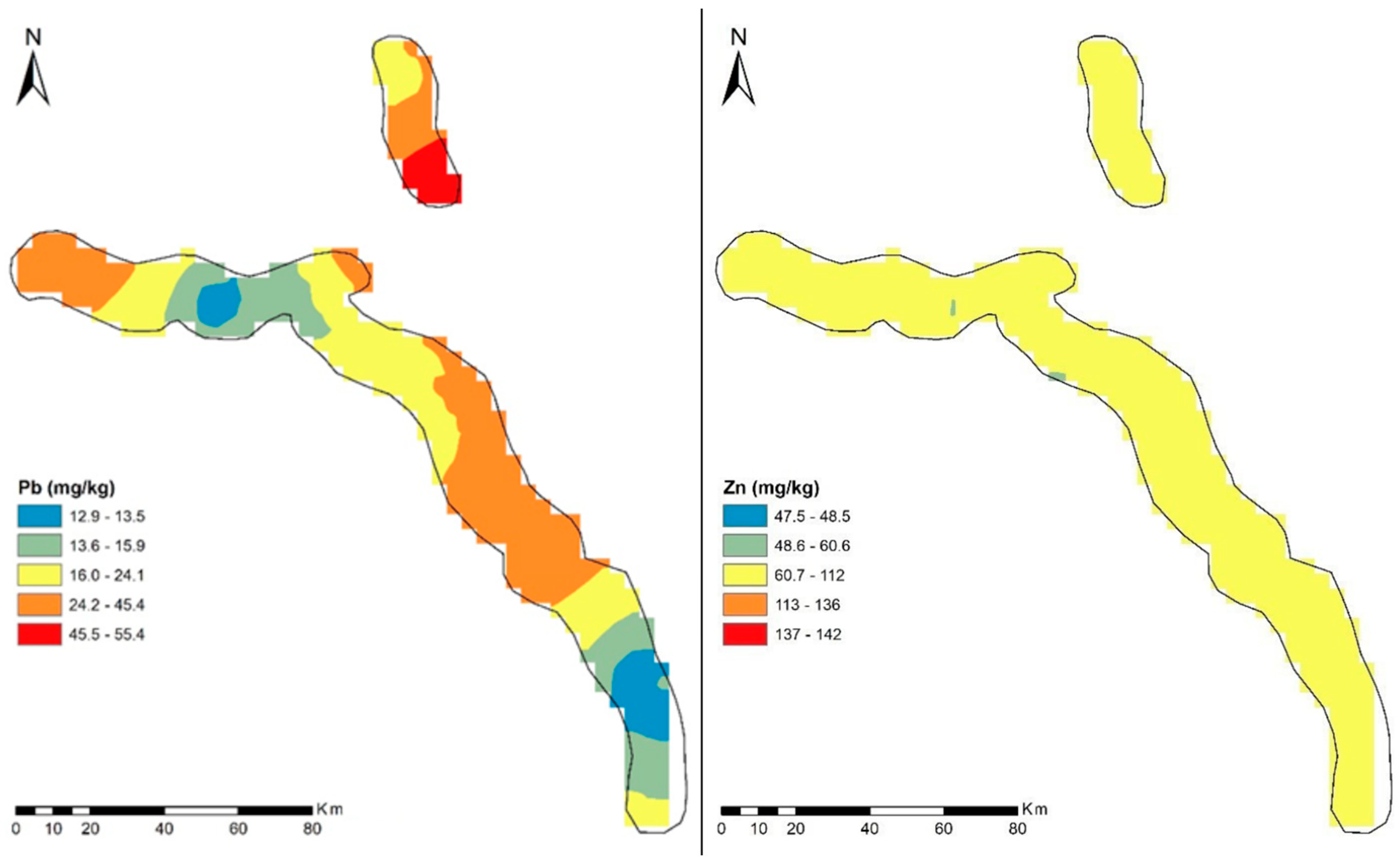
3.7. Spatial Distribution

The spatial distribution (Figure 8, Figure 9 and Figure 10) of the elements under study shows higher concentrations in Area 1. To the North and Northwest, high concentrations of As, Ba, Cu, Hg, Mn, and Ni are observed. These areas correspond to areas of crops, secondary forests, pastures, and scrublands, where the sampling points are located more than 30 m from secondary roads, highways, and the Buena Vista population center. In addition, one of the samples is located within meters of an electrical substation. The soil samples were developed on conglomerates, granite, colluvial alluvial deposits, schists with Cu-Pb-Zn-Ag, and limestones with stratiform bodies of Pb-Zn-Ag.

High concentrations of Ba, Cd, Hg, Mn, and Ni are observed towards the SE of Area 1, where secondary forests, pastures, and crops are developed on granite and limestone. They are located at distances of at least 30 m from high-voltage pylons and secondary roads.

The highest lead concentrations are found to the South of Area 2 in areas of secondary forest or grassland, with one sampling close to a house over limestone lithology with Pb-Zn-Ag stratiform bodies. High concentrations of lead can also be observed in the N, NW, and E of area 1 in areas close to a public road and the Buena Vista village center over limestone and granite lithology.

Cd and Ni also show high concentrations to the South of Area 2 in an area close to the Chinchavito village center. Finally, for Cr and Zn, concentrations are relatively low and mostly concentrated within the 50th and 75th percentiles. It should be noted that the study area is free of industries, and the spatial distribution of the elements under study is based on models associated with the concentrations recorded, which are mostly below the geochemical baseline and EQS values.

4. Conclusions

The estimated geochemical baseline values correspond to Al 34,734 (mg/kg), As 15.3 (mg/kg), Ba 113 (mg/kg), Cd 0.41 (mg/kg), Cr 33.8 (mg/kg), Cu 42.9 (mg/kg), Fe 46,181 (mg/kg), Hg 0.12 (mg/kg), Mn 1015 (mg/kg), Ni 42.2 (mg/kg), Pb 21.6 (mg/kg), and Zn 121 (mg/kg).

Based on the statistical processing and spatial distribution of the data, it is estimated that the concentrations of the elements under study are mainly due to the lithology and geochemistry of the source rock. Even so, it is estimated that other sources could have an influence, due to the use of fertilizers in the areas laid out for agriculture and contamination by vehicular traffic in the areas close to the road and public roads.

The ecological risks calculated with the geochemical baseline values of median ± 2 MAD show that for the geoaccumulation index, enrichment factor, and degree of contamination, only small percentages of the total samples exceed significant thresholds, so 89.7% of the total samples are at a low level of contamination. Similarly, the results obtained with values show that the degree of contamination in 100% of the samples for the elements As, Ba, Cd, Hg, and Pb are at a low level. For non-carcinogenic risks, As and Mn are the elements that represent the highest non-carcinogenic risk in children and adults, so it is recommended to further analyze them to protect people’s health. The carcinogenic risk from As in children represents 3.4% of the total samples. The results of this study are expected to contribute to environmental soil databases that will facilitate the detection of future contamination problems in soils with high technogenic impact and the development of management and remediation strategies for heavy metal-contaminated soils.

References

1. Rodríguez, N.; McLaughlin, M.; Pennock, D. La Contaminación del Suelo: Una Realidad Oculta; FAO: Roma, Italy, 2019; Available online: https://www.fao.org/3/i9183es/i9183es.pdf (accessed on 3 March 2023).
2. Mahecha, J.; Trujillo, J.Y.; Torres, M. Análisis de estudios en metales pesados en zonas agrícolas de Colombia. Orinoquia 2017, 21 (Suppl. S1), 83–93. [Google Scholar] [CrossRef]
3. Targulian, V.O.; Bronnikova, M.A. Soil Memory: Theoretical basics of the concept, its current state and prospects for development. Eurasian Soil Sc. 2019, 52, 229–243. [Google Scholar] [CrossRef]
4. Instituto Nacional de Estadística e Informática [INEI]. Población Peruana Alcanzó las 33 Millones 396 Mil Personas en el año 2022. 2022. Available online: https://www.inei.gob.pe/media/MenuRecursivo/noticias/nota-de-prensa-no-115-2022-inei.pdf (accessed on 3 March 2023).
5. Sánchez, J.; Cubas, N. Contaminación agricolaación por uso de aguas residuales. Alfa Rev. De Investig. En Cienc. Agronómicas Y Vet. 2021, 5, 65–77. [Google Scholar] [CrossRef]
6. Arce, S.; Calderón, M. Suelos contaminados con plomo en la Ciudad de La Oroya-Junín y su impacto en las aguas del Río Mantaro. Rev. Del Inst. De Investig. De La Fac. De Minas Metal. Y Cienc. Geográficas 2017, 20, 48–55. Available online: https://revistasinvestigacion.unmsm.edu.pe/index.php/iigeo/article/view/14389/12724 (accessed on 3 March 2023).
7. Chira, J. Dispersión geoquímica de metales pesados y su impacto en los suelos de la cuenca del río Mantaro, departamento de Junín-Perú. Rev. Del Inst. De Investig. De La Fac. De Minas Metal. Y Cienc. Geográficas 2021, 24, 47–56. [Google Scholar] [CrossRef]
8. Santos, F.; Martinez, A.; Alonso, P.; García, A. Geochemical Background and Baseline Values Determination and Spatial Distribution of Heavy Metal Pollution in Soils of the Andes Mountain Range (Cajamarca-Huancavelica, Peru). Int. J. Environ. Res. Public Health 2017, 14, 859. [Google Scholar] [CrossRef]
9. Soto, M.; Rodriguez, L.; Olivera, M.; Arostegui, V.; Colina, C.; Garate, J. Riesgos para la salud por metales pesados en productos agrícolas cultivados en áreas abandonadas por la minería aurífera en la Amazonía peruana. Sci. Agropecu. 2020, 11, 49–59. [Google Scholar] [CrossRef]
10. Ley Nº 28611, Ley General del Ambiente. 10 April 2005. Available online: https://www.minam.gob.pe/wp-content/uploads/2017/04/Ley-N°-28611.pdf (accessed on 15 May 2023).
11. USEPA. METHOD 3050B-Microwave Assisted Acid Digestion of Sediments, Sludges, Soils and Oils; United States Environmental Protection Agency: Washington, DC, USA, 1996.
12. USEPA. METHOD 6020B-Inductively Coupled Plasma Mass Spectrometry; United States Environmental Protection Agency: Washington, DC, USA, 2014.
13. Bohemen, H.V.; Janssen Van De Laak, W.H. The influence of road infrastructure and traffic on soil, water, and air quality. Environ. Manag. 2003, 31, 0050–0068. [Google Scholar] [CrossRef]
14. Szwalec, A.; Mundała, P.; Kędzior, R.; Pawlik, J. Monitoring and assessment of cadmium, lead, zinc and copper concentrations in arable roadside soils in terms of different traffic conditions. Env. Monit Assess 2020, 192, 155. [Google Scholar] [CrossRef]
15. Consorcio Transmantaro, S.A. Estudio de Impacto Ambiental Detallado para el Proyecto “Enlace 500 kV Nueva Yanango—Nueva Huánuco y Subestaciones Asociadas”. 2019. Available online: https://eva.senace.gob.pe:8443/consultaCiudadano/#/ (accessed on 28 May 2023).
16. Steinmüller, K. Cuadrángulo de la Unión Hoja 20j. Evaluación de Recursos Minerales (Parte de Gabinete). Informe Técnico A6417. INGEMMET: Lima, Peru, 1996. Available online: https://hdl.handle.net/20.500.12544/3938 (accessed on 19 July 2023).
17. Cobbing, E.J.; Quispesivana Quispe, L.Y.; Paz Maidana, M. Geología de los cuadrángulos de Ambo, Cerro de Pasco y Ondores. Boletín, Serie A: Carta Geológica Nacional, n° 77. INGEMMET: Lima, Peru, 1996. Available online: https://hdl.handle.net/20.500.12544/200 (accessed on 19 July 2023).
18. De La Cruz, J.; Valencia, M.; Boulaugger, E. Geología de los cuadrángulos de Aguaytía, Panao y Pozuzo. Boletín, Serie A: Carta Geológica Nacional, n° 80. INGEMMET: Lima, Peru, 1996. Available online: https://hdl.handle.net/20.500.12544/36 (accessed on 19 July 2023).
19. León, W.; Monge, R.; Chacón, N. Geología de los cuadrángulos de Chuchurras, Ulcumayo, Oxapampa y La Merced. Boletín, Serie A: Carta Geológica Nacional, n° 78. INGEMMET: Lima, Peru, 1996. Available online: https://hdl.handle.net/20.500.12544/201 (accessed on 19 July 2023).
20. Martínez, W.; Valdivia, E.; Cuyubamba, V. Geología de los cuadrángulos de Aucayacu, Río Santa Ana y Tingo María. Boletín, Serie A: Carta Geológica Nacional, n° 112. INGEMMET: Lima, Peru, 1998. Available online: https://hdl.handle.net/20.500.12544/71 (accessed on 19 July 2023).
21. Quispesivana, L. Geología del cuadrángulo de Huánuco. Boletín, Serie A: Carta Geológica Nacional, n° 75. INGEMMET: Lima, Peru, 1996. Available online: https://hdl.handle.net/20.500.12544/198 (accessed on 19 July 2023).
22. Fukue, M.; Yanai, M.; Sato, Y.; Fujikawa, T.; Furukawa, Y.; Tani, S. Background values for evaluation of heavy metal contamination in sediments. J. Hazard. Mater. 2006, 136, 111–119. [Google Scholar] [CrossRef] [PubMed]
23. Reimann, C.; Filzmoser, P.; Garrett, R.G. Background and threshold: Critical comparison of methods of determination. Sci. Total Environ. 2005, 346, 1–16. [Google Scholar] [CrossRef] [PubMed]
24. Jarva, J.; Tarvainen, T.; Reinikainen, J.; Eklund, M. TAPIR-Finnish national geochemical baseline database. Sci. Total Environ. 2010, 408, 4385–4395. [Google Scholar] [CrossRef] [PubMed]
25. Maurelia, J.; Cornejo, O.; Tume, P.; Roca, N. Distribution of Heavy Metals in the Commune of Coronel, Chile. Minerals 2022, 12, 320. [Google Scholar] [CrossRef]
26. Ander, E.; Johnson, C.; Cave, M.; Palumbo, B.; Nathanail, C.; Lark, R. Methodology for the determination of normal background concentrations of contaminants in English soil. Sci. Total Environ. Vol. 2013, 454–455, 604–618. [Google Scholar] [CrossRef]
27. Tume, P.; Roca, N.; Rubio, R.; King, R.; Bech, J. An assessment of the potentially hazardous element contamination in urban soils of Arica, Chile. J. Geochem. Explor. 2018, 184, 345–357. [Google Scholar] [CrossRef]
28. Hakanson, L. An ecological risk index for aquatic pollution-control—A sedimentological approach. Water Res. 1980, 14, 975–1001. [Google Scholar] [CrossRef]
29. Müller, G. Index of geoaccumulation in sediments of the Rhine River. Geo J. 1969, 2, 108–118. [Google Scholar]
30. Sutherland, R.; Tolosa, C.; Tack, F.; Verloo, M. Characterization of selected element concentrations and enrichment ratios in background and anthropogenically impacted roadside areas. Arch. Environ. Contam. Toxicol. 2000, 38, 428–438. [Google Scholar] [CrossRef] [PubMed]
31. Fu, C.; Guo, J.; Pan, J.; Qi, J.; Zhou, W. Potential ecological risk assessment of heavy metal pollution in sediments of the Yangtze River within the Wanzhou section, China. Biol. Trace Elem. Res. 2009, 129, 270–277. [Google Scholar] [CrossRef] [PubMed]
32. Marín, J.; Rojas, J.; Polo, C. Evaluación de riesgo ecológico por elementos potencialmente tóxicos en sedimentos costeros de un estuario tropical hipereutrófico. Rev. Int. De Contam. Ambient. 2022, 38, 54504. [Google Scholar] [CrossRef]
33. Tume, P.; Gonzalez, E.; King, R.W.; Monsalve, V.; Roca, N.; Bech, J. Spatial distribution of potentially harmful elements in urban soils, city of Talcahuano, Chile. J. Geochem. Explor. 2018, 184, 333–344. [Google Scholar] [CrossRef]
34. Loska, K.; Wiechuła, D.; Korus, I. Metal contamination of farming soils affected by industry. Environ. Int. 2004, 30, 159–165. [Google Scholar] [CrossRef] [PubMed]
35. Ministerio del Ambiente. Decreto Supremo N.º 011-2017-MINAM; Ministerio del Ambiente: Lima, Peru, 2017; 4p. Available online: https://www.minam.gob.pe/disposiciones/decreto-supremo-n-011-2017-minam/ (accessed on 19 July 2023).
36. USEPA. Risk Assessment Guidance for Superfund Volume I Human Health Evaluation Manual (Part A); Office of Emergency and Remedial Response: Washington, DC, USA, 1989; pp. 1–291. Available online: https://www.epa.gov/sites/default/files/2015-09/documents/rags_a.pdf (accessed on 19 July 2023).
37. USEPA. Guidelines for Exposure Assessment. Risk Assessment Forum; U.S. Environmental Protection Agency Washington: Washington, DC, USA, 1992.
38. USEPA. Supplemental Guidance for Developing Soil Screening Levels for Superfund Sites; Office of Solid Waste and Emergency Response: Washington, DC, USA, 2002.
39. USEPA. Risk Assessment Guidance for Superfund (RAGS); Human Health Evaluation Manual (H. US Epa, 1(540/R/99/005)); USEPA: Washington, DC, USA, 2004; Volume I, pp. 1–156.
40. USEPA; Regional Screening Level (RSL) Resident Soil Table; Varouchakis, Ε.A.; Hristopulos, D.T. Comparison of stochastic and deterministic methods for mapping groundwater level spatial variability in sparsely monitored basins. Environ. Monit. Assess. 2017, 185, 1–19. [Google Scholar] [CrossRef] [PubMed]
41. USEPA. Exposure Factors Handbook: 2011 Edition; National Center for Environmental Assessment Office of Research and Development U.S. Environmental Protection Agency: Washington, DC, USA, 2011; p. 20460.
42. USEPA. Regional Screening Levels (RSLs): Generic Tables (November 2020); USEPA: Washington, DC, USA, 2020.
43. Zheng, N.; Jingshuang, L.; Qichao, W.; Zhongzhu, L. Health risk assessment of heavy metal exposure to street dust in the zinc smelting district, Northeast of China. Sci. Total Environ. 2010, 408, 726–733. [Google Scholar] [CrossRef]
44. Peña, A.; González, M.; Lobo, M. Establishing the importance of human health risk assessment for metals and metalloids in urban environments. Environ. Int. 2014, 72, 176–185. [Google Scholar] [CrossRef]
45. Liu, K.; Shang, Q.; Wan, C. Sources and Health Risks of Heavy Metals in PM2.5 in a Campus in a Typical Suburb Area of Taiyuan, North China. Atmosphere 2018, 9, 46. [Google Scholar] [CrossRef]
46. Frey, P.; Reed, G. The Ubiquity of Iron. ACS Chem. Biol. 2012, 7, 1477–1481. [Google Scholar] [CrossRef] [PubMed]
47. Acosta, J.; Quispe, J.; Santisteban, A.; Acosta, H. Épocas Metalogenéticas y Tipos de Yacimientos Metálicos en la Margen Occidental del sur del Perú: Latitudes 14°s–18°s. En: Congreso Peruano de Geología, 14, Congreso Latinoamericano de Geología, 13, Lima, PE, 29 Setiembre–3 Octubre 2008, Resúmenes; Sociedad Geológica del Perú: Lima, Peru, 2008; 6p, Available online: https://hdl.handle.net/20.500.12544/424 (accessed on 19 July 2023).
48. Agencia Para Sustancias Tóxicas y el Registro de Enfermedades [ATSDR]. Reseña Toxicológica del Arsénico (Versión Para Comentario Público) (en Inglés); Departamento de Salud y Servicios Humanos de EE. UU., Servicio de Salud Pública: Atlanta, GA, USA, 2005. Available online: https://www.atsdr.cdc.gov/es/phs/es_phs2.html (accessed on 19 July 2023).
49. Romero, K.; Martínez, O. Análisis factorial exploratorio mediante el uso de las medidas de adecuación muestral kmo y esfericidad de bartlett para determinar factores principales. J. Sci. Res. (CININGEC) 2020, 5, 903–924. Available online: https://revistas.utb.edu.ec/index.php/sr/article/view/1046 (accessed on 19 July 2023).
50. Sánchez, E.; Sarria, K. Papel del Suelo en la Toxicidad del Cadmio. Ph.D. Thesis, Universidad Complutense, Madrid, Spain, 2017. Available online: https://eprints.ucm.es/id/eprint/56981/1/ELENA%20SANCHEZ%20LEON.pdf (accessed on 19 July 2023).
51. Machado, A.; Velázquez, H.; García, N.; García, C.; Acosta, L.; Córdova, A.; Linares, M. Metales en PM10 y su dispersión en una zona de alto tráfico vehicular. Interciencia 2007, 32, 312–317. Available online: http://ve.scielo.org/scielo.php?script=sci_arttext&pid=S0378-18442007000500006&lng=es&tlng=es (accessed on 19 July 2023).
52. Carlon, C. (Ed.) Derivation Methods of SOIL Screening Values in Europe—A Review and Evaluation of National Procedures towards Harmonization; European Commission, Joint Research Centre: Ispra, Italy, 2007. [Google Scholar]
Figure 1. Location of samples collected in surface soil (0–25 cm).
Minerals 14 00546 g001
Figure 2. Correlation between the different lithostratigraphic units and the different departments in the study area.
Minerals 14 00546 g002
Figure 3. Dendrograms of cluster analysis, using Ward’s method, of heavy metals in surface soil (0–25 cm) of the project.
Minerals 14 00546 g003
Figure 4. Threshold values and soil sample distribution for As, Ba, Cd, Hg, and Pb with EQS values and geochemical baseline values by median method.
Minerals 14 00546 g004
Figure 5. Box-plot diagram for ecological indices using geochemical baseline values using the median ± 2 MAD method. The red dashed lines point out the classification of each environmental index.
Minerals 14 00546 g005
Figure 6. Box-plot plots for the ecological indices using the EQS values for agricultural land use as generic reference values.
Minerals 14 00546 g006
Figure 7. Box-plot diagrams for carcinogenic and non-carcinogenic risks in children and adults.
Minerals 14 00546 g007
Figure 8. Spatial distribution of As, Ba, Cd, and Cr concentrations (mg/kg).
Minerals 14 00546 g008
Figure 9. Spatial distribution of Cu, Hg, Mn, and Ni concentrations (mg/kg).
Minerals 14 00546 g009
Figure 10. Spatial distribution of Pb and Zn concentrations (mg/kg).
Minerals 14 00546 g010