Article

Inversion of TEM Responses in Tunnel with Steel Infrastructure and Its Application

1
School of Information Science and Engineering, China University of Petroleum (Beijing), Beijing 102249, China
2
School of Geophysics, China University of Petroleum (Beijing), Beijing 102249, China
3
State Key Laboratory of Petroleum Resources and Prospecting, China University of Petroleum (Beijing), Beijing 102249, China
4
Bureau of Geophysical Prospecting, China National Petroleum Corporation, Zhuozhou 072751, China
*
Author to whom correspondence should be addressed.
Minerals 2024, 14(8), 802; https://doi.org/10.3390/min14080802 (registering DOI)
Submission received: 22 June 2024 / Revised: 29 July 2024 / Accepted: 3 August 2024 / Published: 7 August 2024

Abstract

:
Steel infrastructure in tunnels significantly affects the accuracy of transient electromagnetic (TEM) data inversion. This study proposes and compares two methods to effectively mitigate this interference: the correction factor method and the prior information constraint method. The correction factor method constructs correction factors using interference data obtained in two ways. The first method, numerical simulation, is theoretically precise but relies heavily on accurate model parameters and requires significant computational resources. The second is conducted by measuring the interference data in the working space. While this approach is simple and operationally convenient, its effectiveness in correction is limited by the measured data quality. The a priori information constraint method improves the inversion by introducing a more accurate initial model. The inversion results of synthetic data indicate that the inversion based on the correction factor method and the prior information constraint method can effectively invert the anomaly. However, the delay effect remains a challenge for the correction factor method. Finally, we invert the field data measured in a mine tunnel by combining the interference processing methods.

1. Introduction

The transient electromagnetic method (TEM) is extensively used in mineral exploration [1,2], hazard prediction [3,4], and hydrogeophysics [5,6]. The TEM offers high sensitivity to low-resistivity bodies, ease of implementation, and independence from topography. However, when applied in tunnels, TEM data often suffer from significant interference from steel infrastructure such as supports and rails. This steel infrastructure significantly impacts data quality and poses challenges for inversion, necessitating effective interference mitigation techniques to enhance inversion accuracy.
Although the TEM is highly sensitive and advantageous for detecting low-resistivity anomalies, this high sensitivity also makes it more susceptible to high-conductivity interference [7,8]. Numerous studies have demonstrated that the proximity of steel infrastructure to measurement stations can cause substantial distortions in electromagnetic fields [9,10,11,12,13]. This interference considerably affects the accuracy of inversion results in environments with strong disturbances, such as water inrush detection in mine tunnels [14,15]. Geological predictions in tunnel excavation are susceptible to surrounding high-conductivity interference, which leads to low accuracy in inversion interpretation [16]. In these cases, interference and effective signals are intertwined and cannot be directly separated in the time or frequency domains. Traditionally, methods such as constructing correction factors, initially developed to correct the geomagnetic and marine electromagnetic topography [17,18], have been adapted to address metal interference in tunnel TEM data [19,20]. This involves generating correction factors from actual measurements obtained with and without interference. However, the quality of the actual measured interference response cannot be guaranteed owing to the influence of various noises in the tunnel, and the constructed correction coefficients lack accuracy. Therefore, some scholars have examined the interference response through numerical simulations to obtain a more accurate interference response. With numerical simulation algorithms and computer equipment development, three-dimensional modeling, which discretizes the subsurface space into numerous small cells, has been developed to simulate arbitrarily complex geology [21]. The response characteristics of a power line and steel casing were analyzed using high-precision numerical simulations [22,23]. This suggests the potential to discretize steel infrastructure using small cells and analyze their response characteristics through numerical simulations. Therefore, incorporating the interference factor into the initial inversion model as a known factor is a feasible approach. In some cases, if additional prior information about the subsurface is available, it can be incorporated into the inversion to obtain more accurate and realistic results [24].
Our algorithm was developed based on simulations and parameter estimation in geophysics (SimPEG) [25,26]. SimPEG is an open-source Python framework designed for forward simulations and parameter inversion in geophysics. We first analyzed the impact of inversion effects before and after interference processing and confirmed the necessity of such processing. Subsequently, we used synthetic data to assess the feasibility of interference-processing methods. Finally, the field data collected in a coal mine tunnel were inverted.

2. Methods

2.1. Forward and Inversion Theory

During the forward simulation, the electromagnetic response of the subsurface medium is modeled by solving Maxwell’s equations [25,26].
× e + b t = s m ,
× μ 1 b σ e = s e ,
where e is the electric field; b is the magnetic flux density; s m is the magnetic source term; s e is the electric source term; and μ and σ are magnetic permeability and electrical conductivity, respectively.
An inversion algorithm from the SimPEG framework minimizes the objective function [26,27]. Optimization techniques, such as the gradient descent and conjugate gradient methods, are employed to determine the optimal conductivity distribution.
m = arg min m W d d o b s d p r e d 2 2 + β W m m m r e f 2 2 ,
where β is an adjustable trade-off parameter; m and m r e f are the model solution and reference model, respectively; W d is a diagonal matrix; W m is the model weighting matrix; and d p r e d and d o b s are the predicted and observed data of N d × n c h a n n e l dimensions, respectively. N d is the number of measurement stations, while n c h a n n e l is the number of time channels.

2.2. Data Pre-Processing Methods

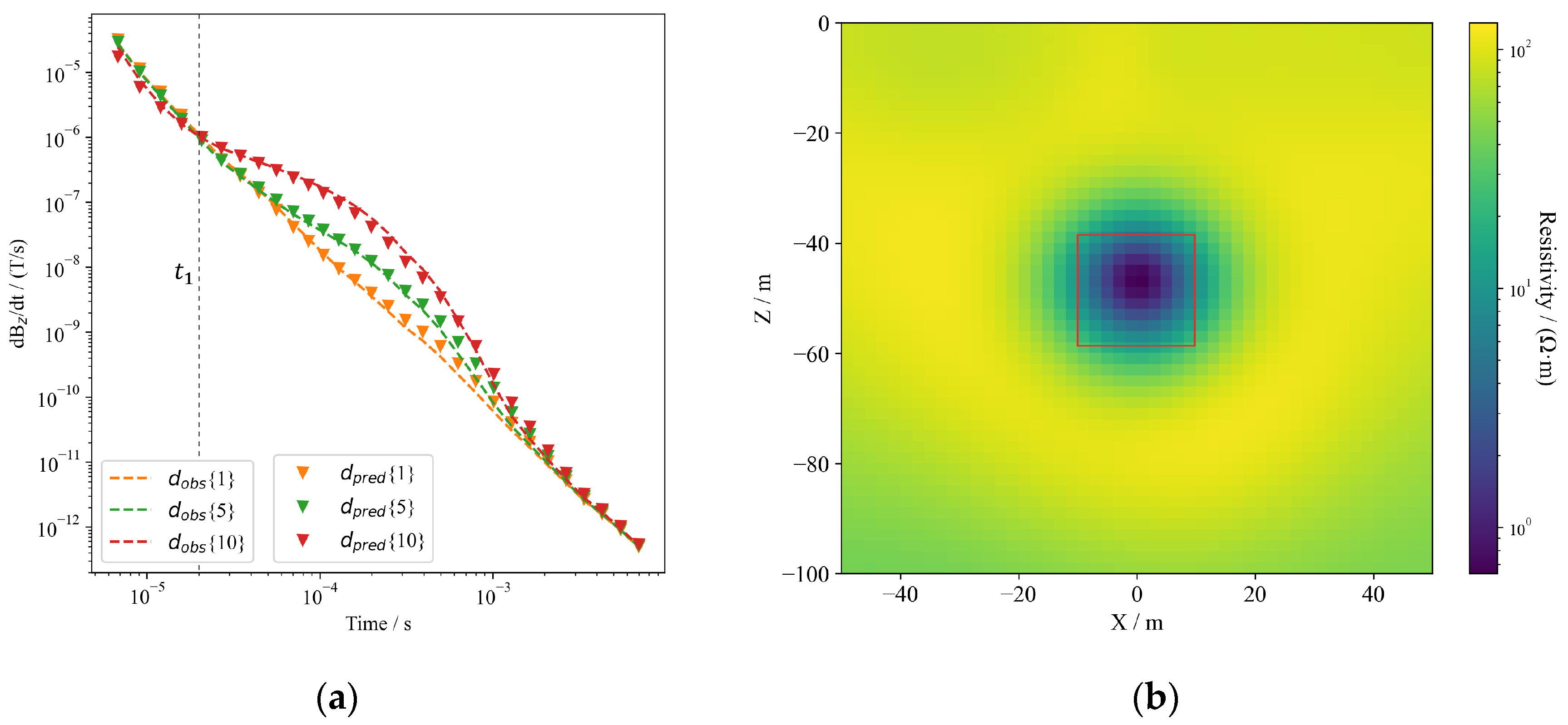
To analyze the effect of low-resistivity interference on inversion interpretation and demonstrate the necessity of data preprocessing, we used the model shown in Figure 1 to calculate the simulated data with and without interference. This study only focuses on a simple model, although the interference in an actual tunnel is considerably more complex. We set the resistivity and thickness of the interference to 1 Ω∙m and 2 m in this model. Twenty measurement stations were established, with 5 m spacing between every two stations. We used data from 20 measurement stations to perform the two-dimensional (2D) inversion jointly. The data fitting curves for each measurement station are not compared; instead, the data fitting curves for Station 1, Station 5, and Station 10 are presented.
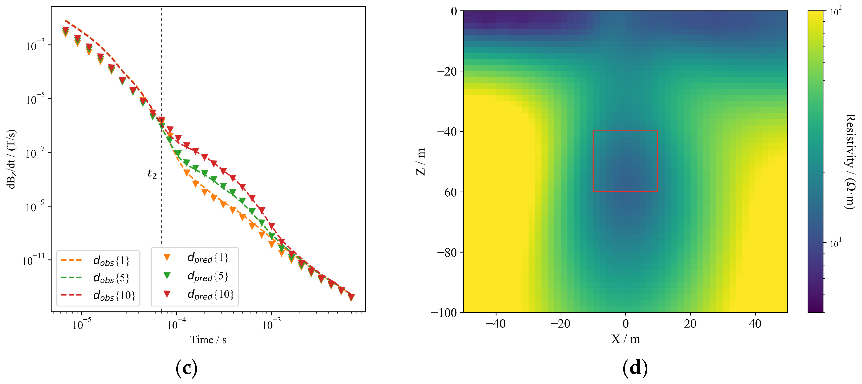
Figure 2 illustrates the inversion results for the simulated data with and without interference. In Figure 2a,c, t1 and t2 represent the beginning moments of the target anomaly’s response characteristics in the absence and presence of interference, respectively. The red box in Figure 2b,d indicates the location of the actual anomaly. The inversion begins with a uniform background medium with a resistivity of 100 Ω · m . To validate the accuracy of the inversion algorithm, we first performed an inversion test on data without interference. Figure 2a shows the dobs and dpred values, depicting the simulated data from the model shown in Figure 1a and the simulated data from the inversion model in Figure 2b, respectively. The response curves in Figure 2a demonstrate a good fit in the absence of interference. Figure 2b depicts that the anomaly distribution in the resistivity profile closely matches that of the actual model, indicating the accuracy and reliability of the inversion algorithm.
The inversion results of the simulated data from the model illustrated in Figure 1b are shown in Figure 2c,d. Figure 2c shows the dobs and dpred values, depicting the simulated data from the model shown in Figure 1b and the simulated data from the inversion model in Figure 2d, respectively. As illustrated in Figure 2c, the data predicted by the inversion model exhibited a poor fit with the observed data at an early stage. Figure 2d reveals a significant deviation from the actual model when the interference is unprocessed. These experiments indicate that interference near the measurement station has a significant impact. If the interference is not considered, it is difficult to reveal the true resistivity distribution of the subsurface medium. To improve the accuracy of the inversion interpretation, we introduce two pre-processing methods to process the interference.

2.2.1. Correction Factor Method

The central idea of the correction factor method is to compare the electromagnetic response with and without interference and calculate the ratio of the two [18,20,28].
K t = d n o _ int t d int t ,
where d int t represents the data with interference, d n o _ int t represents the background response without interference, and K t represents the correction factor.
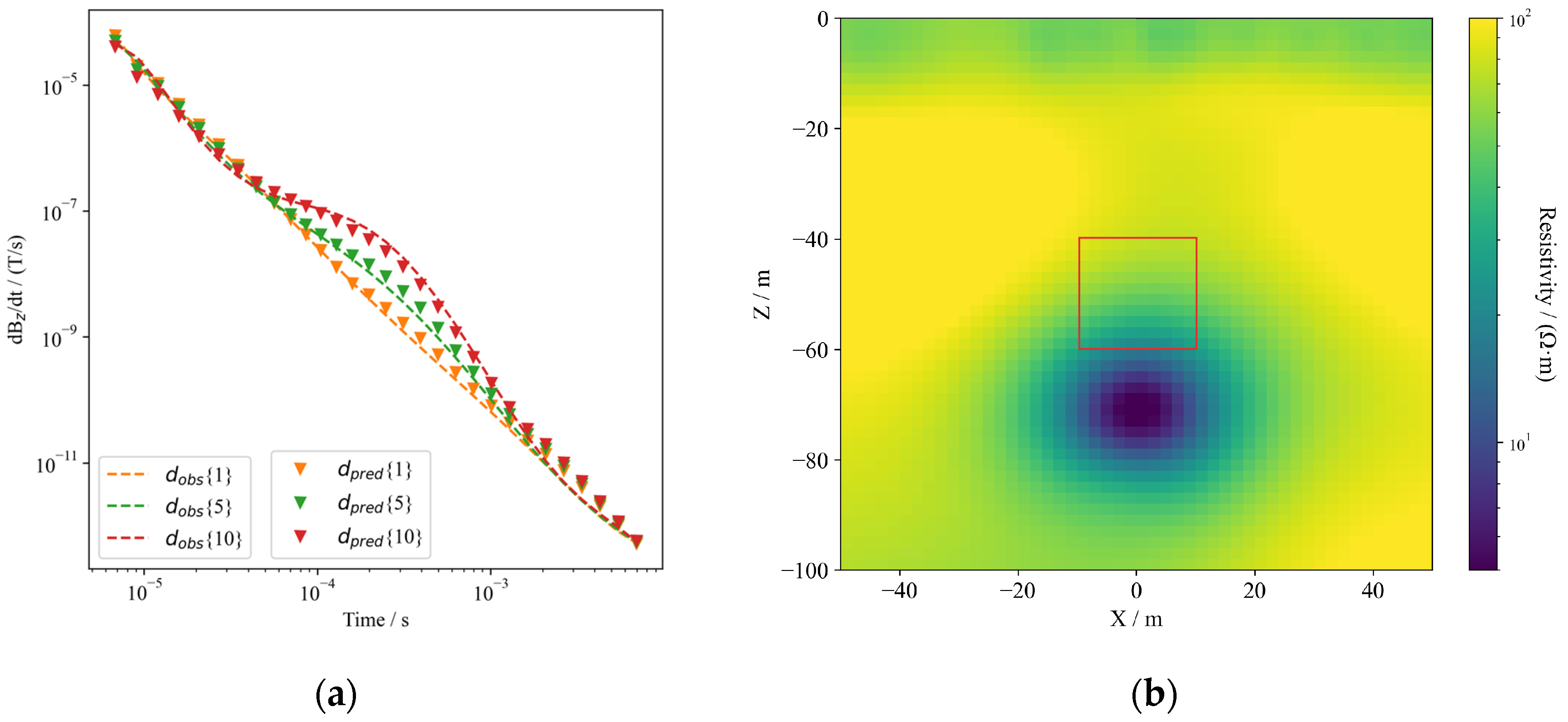
The inversion results obtained by employing the correction factor method to process the interfering data are shown in Figure 3. The background resistivity of the initial inversion model is 100 Ω · m . Figure 3a shows the observed data after correction and predicted data from the inversion model. As shown in Figure 3b, the interpretation accuracy of the inversion results improved after correction. However, the position of the anomaly is displaced. This phenomenon occurs because of the delayed effect of the interference layer, which causes a delayed arrival time for the effective response.
To address the issue, we propose a time-shift correction method. This method calculates the background response, d n o _ int , using a forward-shifted time series.
K t = d n o _ int t τ d int t ,
where τ denotes the time shift. However, no simple formula can be used to calculate the time shift, τ , in all cases, and τ remains an empirical parameter. Electromagnetic interference is influenced by several parameters. These parameters include the conductivity, size, shape, location, dielectric constant, magnetic permeability, and frequency of the interfering object. For example, steel has a high magnetic permeability and electrical conductivity, and electromagnetic fields propagate more slowly in steel. Both primary and secondary fields are delayed by steel interference. Additionally, the presence of multiple interfering sources further complicates the accurate determination of τ . If there are several steel structures in close proximity, their combined effects can result in overlapping delays, increasing the complexity of accurately assigning a single delay value.
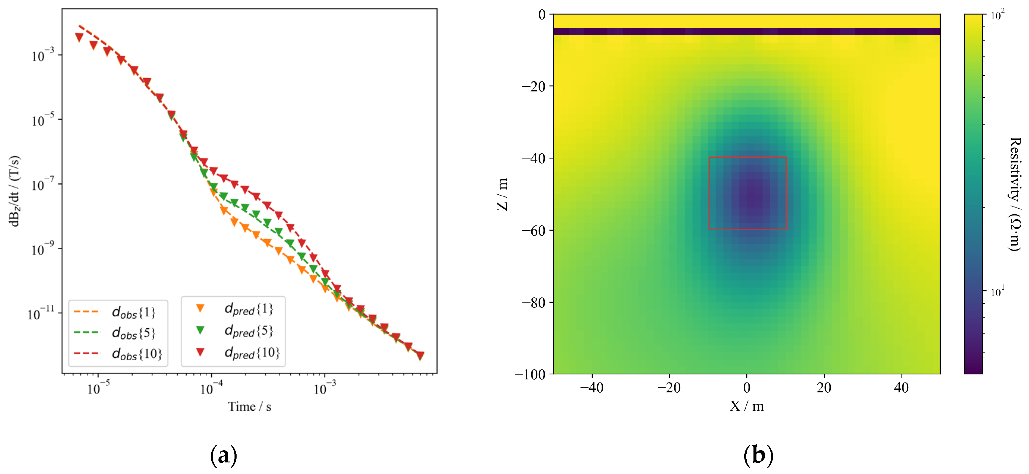
The results of the time-shift correction are shown in Figure 4. We determine the time shift for each timestep here by simply comparing the beginning times of the anomaly response characteristics. The beginning times in Figure 2a,c are known to be t1 and t2. Assuming the original sampling time is T, the two beginning times allow us to determine the new sampling time T n o _ i n t = t 1 / t 2 T for computing d n o _ int . Figure 4a depicts that the corresponding time for the corrected response is advanced. The data predicted by the inversion model fit the corrected data well. Figure 4b shows that the location and size of the target anomaly closely correspond to the actual model. This indicates that the time-shift correction is feasible.
These numerical experiments have demonstrated that the correction factor method can mitigate interference to a certain extent. However, for signal delays caused by high-conductivity interference, incorporating a time-shift correction may be necessary to obtain more accurate results. However, the absence of a unified calculation method for time-shift limits its practical application.

2.2.2. Prior Information Constraint Method

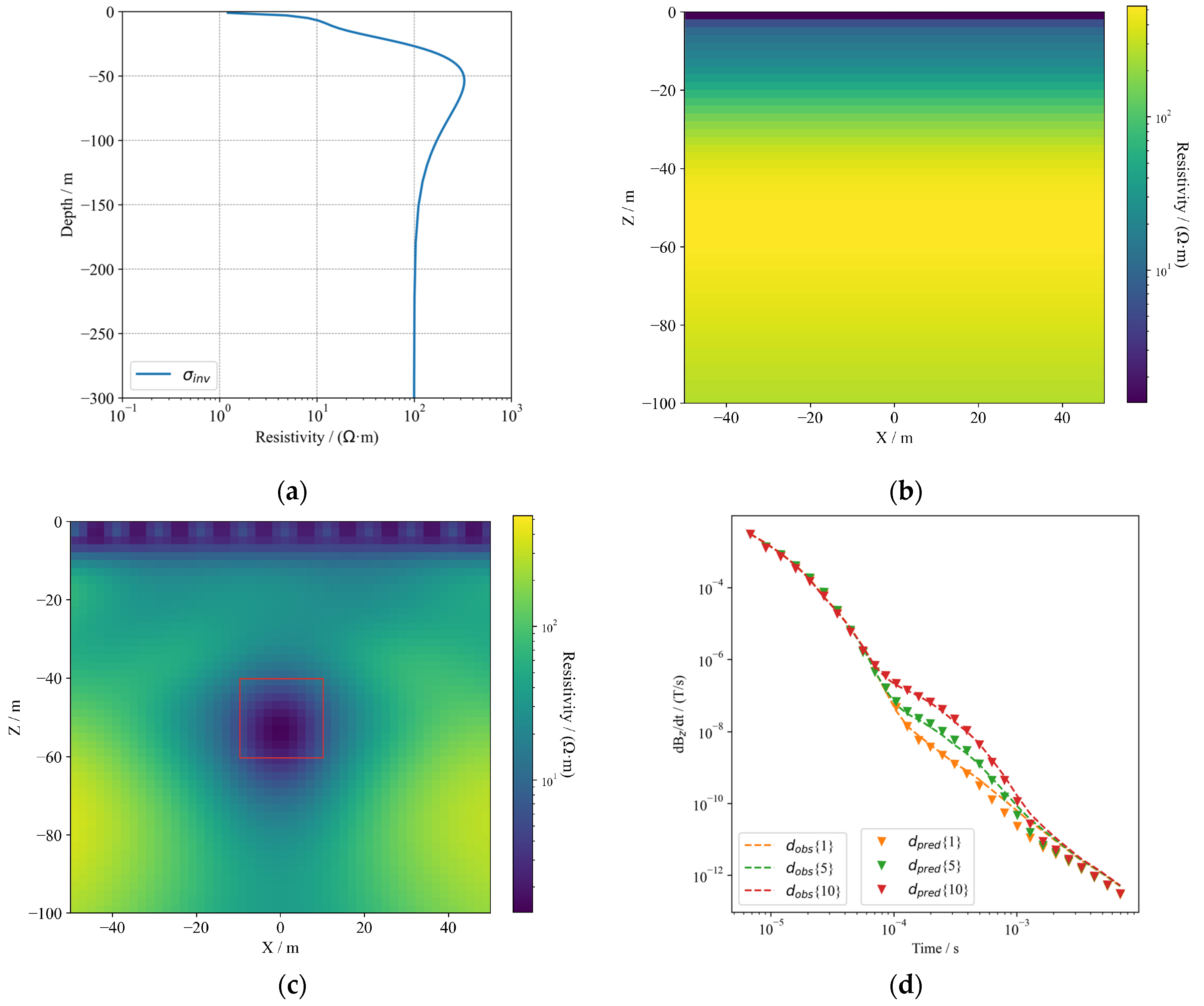
The prior information constraint method (PICM) employs an initial model that incorporates interference factors from known information, such as the spatial distribution and electrical parameters of the interference. This method considers the impact of interference on the target geological body. To examine the effect of the PICM, we use the synthetic data obtained from the model in Figure 1b. With a known interference, researchers can incorporate it into the initial inversion model. Figure 5 illustrates the effect of incorporating the interference factor as a known condition into the initial model. The inversion results show that the PICM-based inversion can effectively invert the anomaly.
When the interference is unknown or difficult to model, the interference data can be processed using a one-dimensional (1D) inversion technique. This method generates a 1D effective model of the interference. This model is subsequently mapped to 2D, becoming the initial model for 2D inversion. This process enables the inversion method to gradually approximate the real interference, even without a full understanding of the interference conditions. Figure 6a shows a 1D inversion result using data from Station 1 in Figure 1b, which results in an effective 1D model of the interference. Figure 6b shows the mapping of the 2D model. This model was used as the initial model for the 2D inversion. Figure 6c shows the resistivity profile obtained from the 2D inversion. The target anomaly can be accurately inverted, and Figure 6d shows a good fit between the observed and predicted responses. Unlike the correction factor method, this approach does not require time-shift correction, further ensuring the reliability of the data interpretation.

3. Field Data Application

3.1. Geological Setting

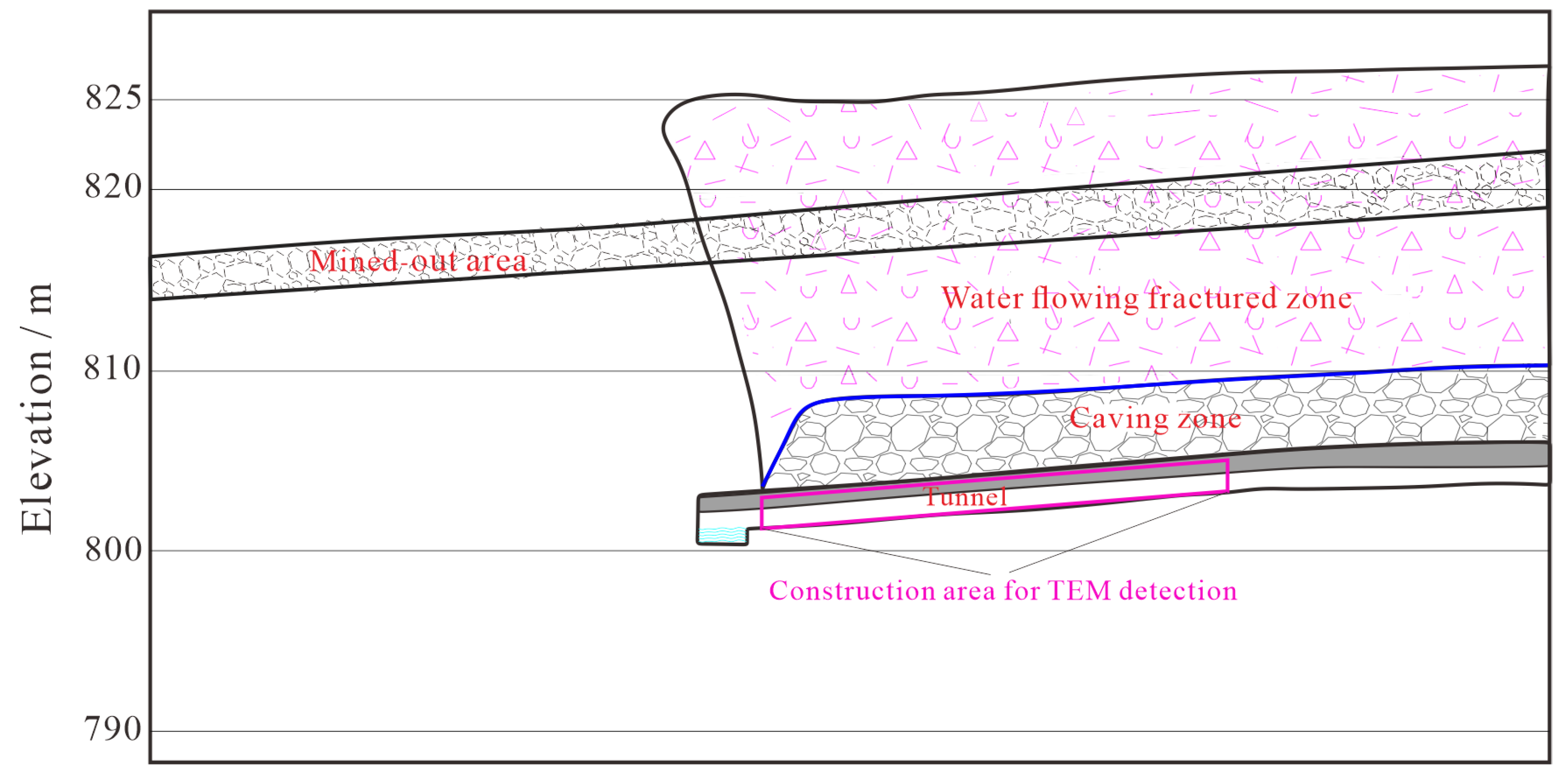
The study’s data were collected from a coal mine tunnel in Lvliang, Shanxi Province, China, at an average depth of 250 m below ground. The underground mining tunnel and its surrounding geological changes are shown in Figure 7. A mined-out area exists above the tunnel. The water in this mined-out area is a potential security risk for the construction tunnels. When a coal seam is extensively excavated, the surrounding rock layers lose their balance, deform, and move owing to gravity. Subsequently, from bottom to top, the overlying strata in the goaf area stabilize, forming caving and fracture zones as shown in Figure 7. The fractured rock layers increase water permeability, creating a water-flowing fracture zone above the tunnel. Sudden water-inrush accidents under the influence of stratum pressure pose significant hidden dangers to construction safety. Therefore, the main targets for TEM detection in mine tunnels are the water-rich zones.

3.2. Interference Analysis

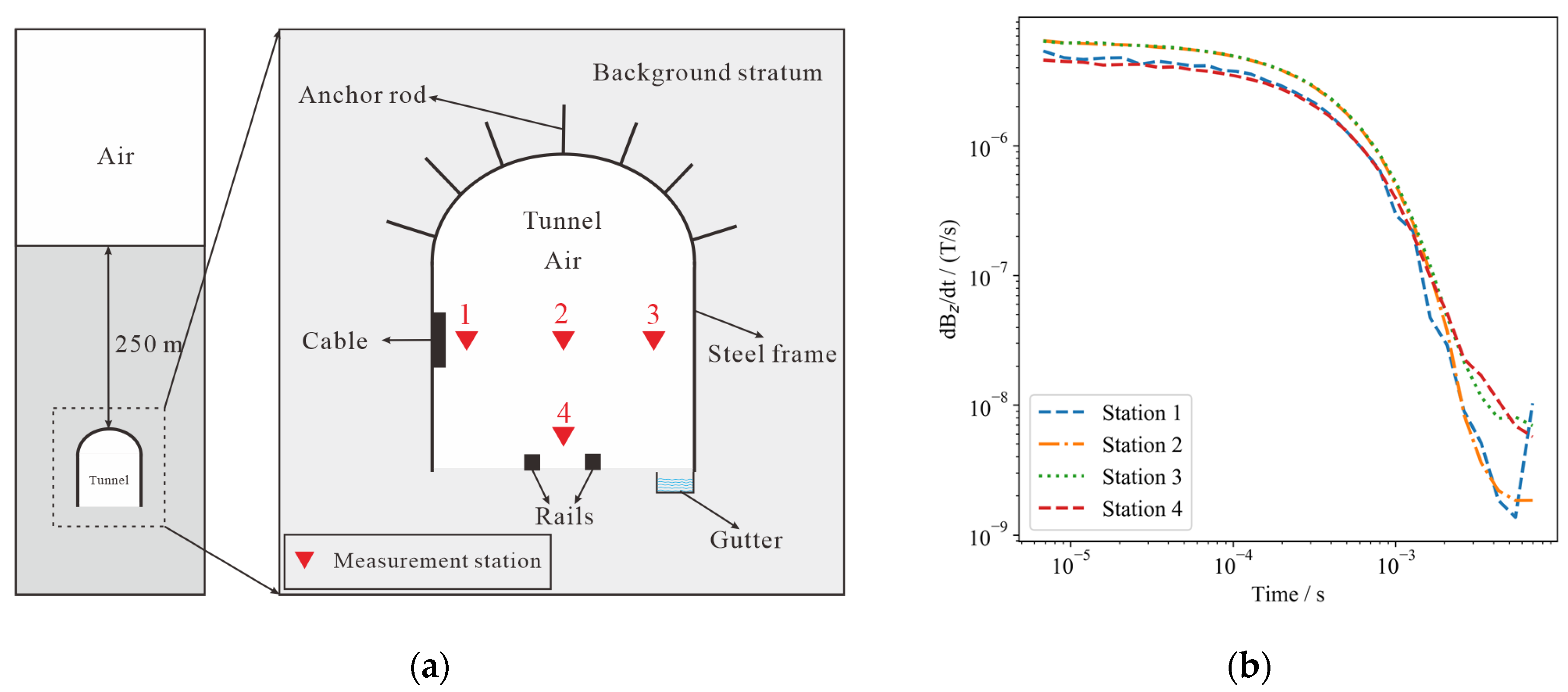
The interference in the tunnel is primarily from the steel infrastructure, such as rails, mining equipment, support structures, and cables. Figure 8a illustrates the distribution within the tunnel. To examine the effect of interference in the tunnel on TEM detection, measurements were conducted at four stations.
Figure 8b displays the measured responses. Under the influence of the interferences, the data from each measurement station decay slowly in the early stage. Specifically, the presence of cables at Station 1 results in severe industrial electrical interference, which distorts the TEM response. Stations 2 and 3, which were farther from the interfering object, experienced lower levels of interference. Their response curves initially overlapped; however, the late response of Station 3 was stronger owing to the closer proximity to the steel frame. The response of Station 4 shows a much slower decay. From the interference survey results, it is suggested that the coil for the actual measurement should be kept at a distance from the steel infrastructure and that locating the measurement station at the tunnel center is a better choice.

3.3. Data Acquisition

The TEM, radio wave imaging (RWI), and drilling methods are utilized in this exploration area. Figure 9a depicts the distribution of the TEM and RWI measurement stations. The hydrogeological anomalies identified by the RWI and boreholes are also depicted in Figure 9a, serving as a cross-validation of the TEM inversion results. The RWI typically uses one transmitter and one receiver, with a transmitting station set up in one tunnel to transmit electromagnetic wave signals and a receiving station in another tunnel to receive these signals [29,30]. The RWI determines the characteristics of underground media based on the difference in the attenuation of high-frequency radio electromagnetic waves as they propagate through various media.
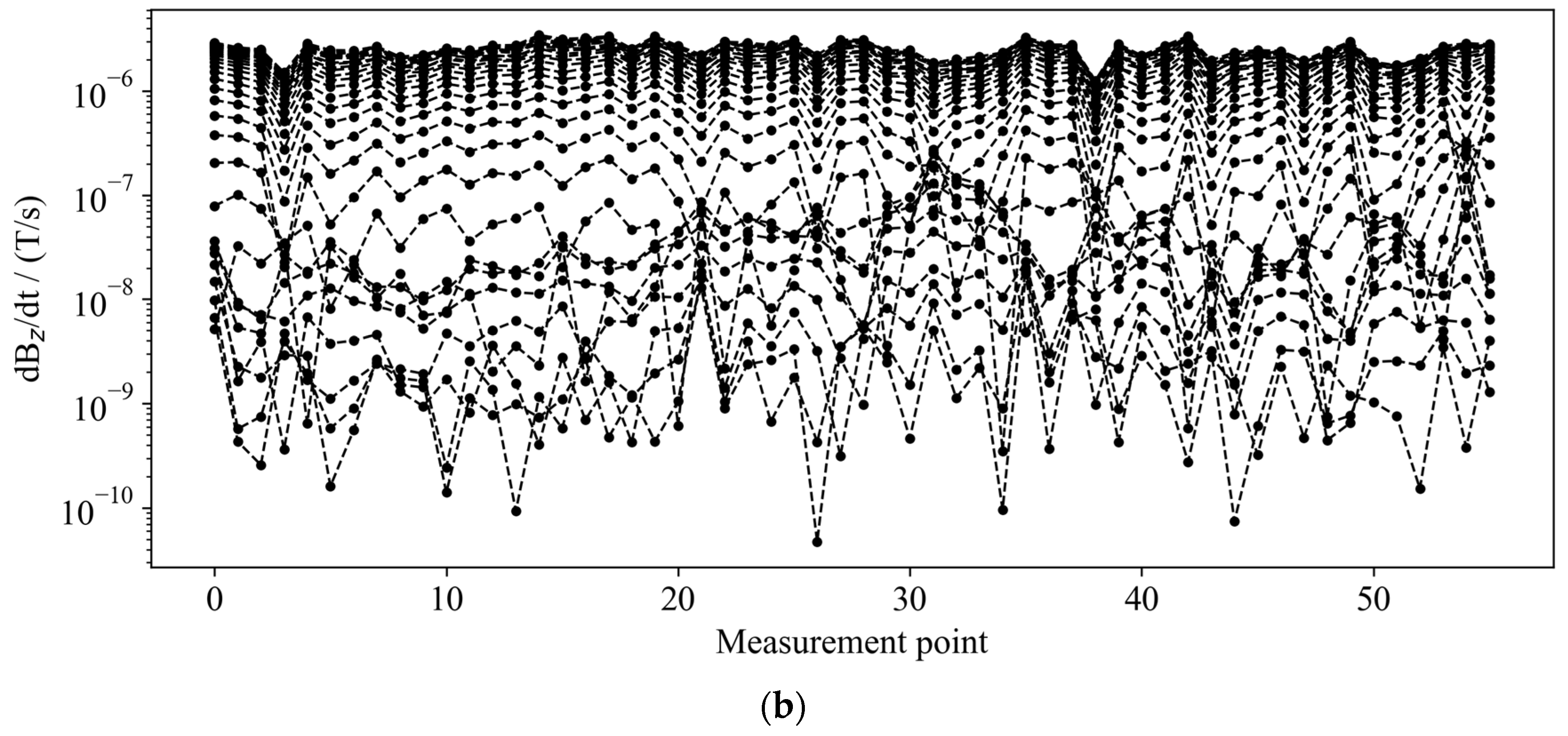
As illustrated in Figure 9a, the TEM survey line is placed along the tunnel center, and the spacing between the measurement stations is 10 m. The total number of TEM measurement stations is 56, and the acquisition device is the PROTEM47. The transmitter is a 1 m × 1 m square coil, and the receiver is a circular coil with a radius of 0.5 m. The decay of the magnetic field is recorded over 30 time gates in the range of 6.8 μs to 5 ms. Due to the limited space in tunnels, often only one survey line can be arranged. In actual measurements, multiple angles are usually conducted to increase the accuracy. Here, we selected the measurement data for the inversion where the detection direction is at an angle of 50° to the tunnel floor. Figure 9b shows the measured response in the mine tunnel.

4. Results and Discussion

In the data processing, we applied two methods to manage the electromagnetic responses in tunnels affected by steel infrastructure: the correction factor method and the PICM. To distinguish between these approaches, we refer to them as the simulation correction method (SCM) and the measured correction method (MCM), respectively. The correction factor is constructed using the interference data obtained from numerical simulations and actual measurements.
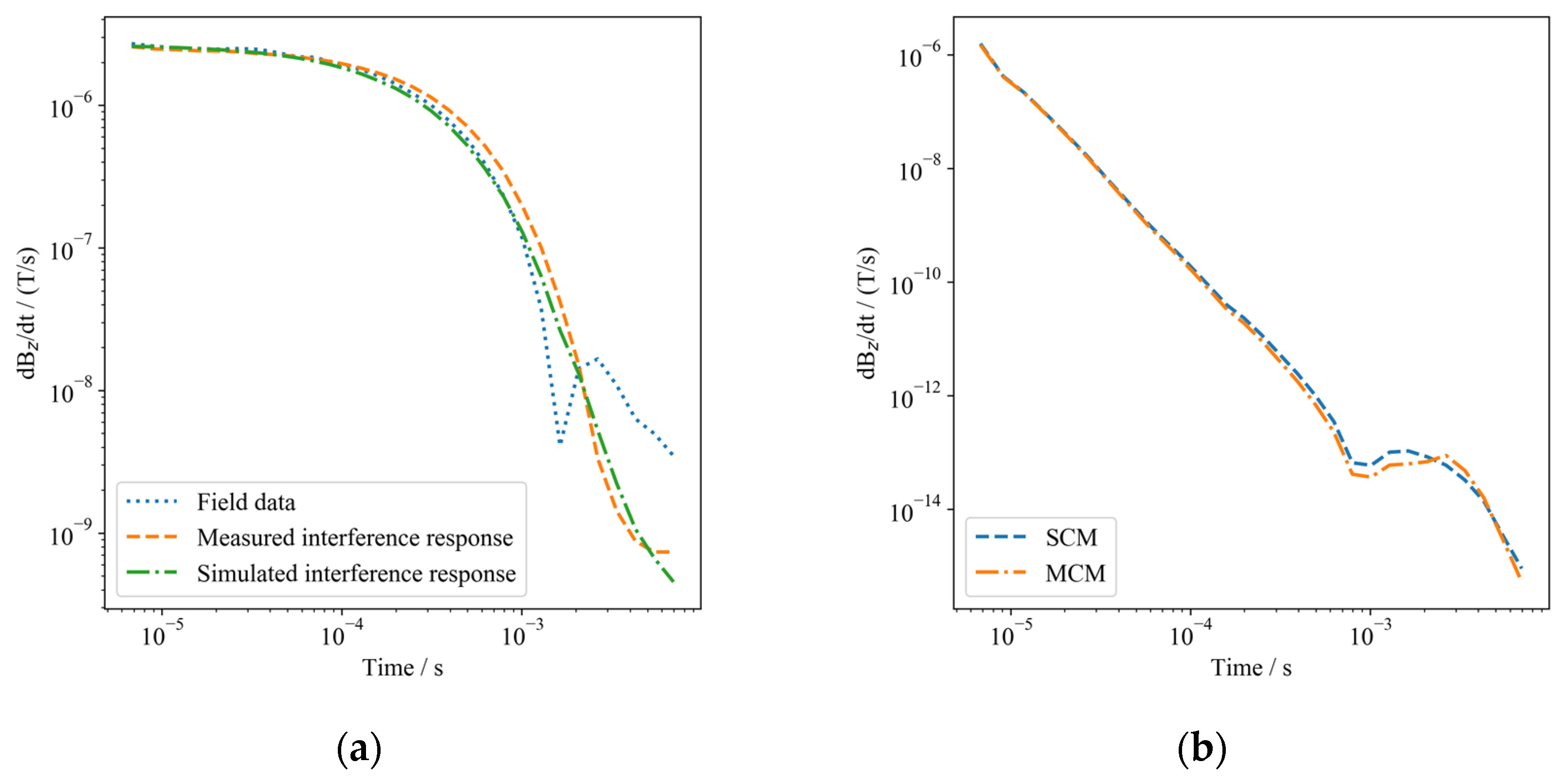
The SCM obtains highly accurate interference response data by precisely controlling the model parameters. We design a model based on the actual situation in a mining tunnel, as shown in Figure 10. The parameters for the tunnel and steel infrastructure are shown in Figure 10a. The cross-sectional area of steel infrastructure is 0.2 m × 0.2 m. The resistivity of the steel infrastructure is set to 10−6 Ω∙m, and the magnetic permeability is set to 100 μ0. An octree grid is used to discretize the model (Figure 10b). Discretization using only small cells at the edges of the tunnel reduces the total number of cells. To ensure simulation accuracy, refined discretization was performed at the transmitter and receiver locations.
The interference data were processed using the SCM and MCM, and the results are shown in Figure 11. Figure 11a depicts the simulated and measured interference responses. We used the interference data from Station 2 (Figure 8b) to implement the MCM. Using Equation (4) to compute the correction factor requires both the interference and non-interference background responses. Ensuring that the measurement area is free from interference is difficult. Therefore, this study employs a numerical simulation to calculate the background response without interference. The results of the above two methods for correcting the field data are shown in Figure 11b.
Figure 12 illustrates the resistivity profile obtained from the inversion of the field data without any interference processing. The high-resistivity areas shown in Figure 12 can be considered as the tunnel, while the low-resistivity areas could result from a combination of interference within the tunnel and actual anomalies in the strata. The influence of interference leads to a widespread distribution of low-resistivity areas in the profile, making it difficult to accurately distinguish actual anomalies. These widely distributed low-resistivity areas increase the complexity of data interpretation, suggesting that further processing of interferences is required in practical applications to more accurately identify actual geological anomalies.
The inversion results based on the correction factor method are shown in Figure 13. Since the simulated and measured interference responses are approximate (Figure 11a), the difference between the inversion results based on the SCM and MCM is small. To verify the accuracy of the inversion results, we used the RWI and borehole survey results for comparison, which are represented in Figure 13 using dotted lines. The inversion results are further improved in accuracy after the interference processing using the correction factor method compared to the inversion result in Figure 12. This demonstrates the effectiveness of the SCM and MCM in processing field data. Compared with the SCM, the MCM features a straightforward measurement process. This eliminates the need for high-precision numerical simulations and reduces computational effort.
The factors affecting the practical effectiveness of the correction factor method are as follows. The accuracy of the SCM depends on the accurate setting of the model parameters, but it is difficult to obtain these parameters in practical applications. The effectiveness of the MCM depends on the quality of the measured interference data. However, the actual measured interference responses are susceptible to various types of noise, making it difficult to ensure data quality. In addition, we used a uniform correction factor for all measurement stations. Although consistency exists in the interference to TEM detection in the tunnels, there may be a stronger interference level at some measurement stations. This results in a spurious anomaly in the inversion results at these measurement stations.
Figure 14a displays the inversion result obtained using the PICM alone. This result shows that in the presence of high-conductivity interference, the PICM-based inversion does not accurately reflect the actual geological situation. Furthermore, the accurate reconstruction of the location and size of anomalies remains challenging. This suggests that for data affected by high-conductivity interference, using a combination of the correction factor method and PICM may be necessary. The inversion result obtained by combining the MCM and PICM is shown in Figure 14b. A 1D inversion was first performed on the corrected data at measurement Station 10 (Figure 9a). The result from the 1D inversion was then mapped to 2D, serving as the initial model for the subsequent 2D inversion. The inversion results for the PICM combined with the MCM provide more details compared to using the PICM alone. Moreover, the spurious anomalies in Figure 13 are suppressed to some extent. Although the inversion yields low-resistivity anomaly areas that are farther away than the circled areas, it still provides a good indication of the distribution of the anomalies.

5. Conclusions

The correction factor method effectively mitigates the interference effect through numerical simulations and actual measurements. However, accurately obtaining model parameters with the SCM is challenging, and the MCM is limited by field conditions and data noise. Additionally, inversion experiments using synthetic data demonstrate that the correction factor method failed to recover the delay caused by interference. This results in the inverted anomaly being farther from the actual anomaly. Although combining the correction method with the time shift can eliminate interference and restore the delay effect, there is no uniform formula for determining the amount of time shift. This limitation restricts the use of the time-shift correction method. Therefore, we introduce the PICM to improve the inversion of disturbed data. The inversion results from the synthetic data indicate that the PICM-based inversion accurately inverts the anomaly. To further validate the effectiveness of these methods, we conduct field data and cross-validate the results using the RWI and boreholes. The inversion results demonstrate that the inversion based on the correction factor method can effectively identify the anomalies. In contrast, using the PICM-based inversion alone performs poorly, and it is difficult to identify the distribution of anomalous areas. This suggests the limited applicability of using the PICM-based inversion alone. For data significantly affected by high-conductivity interference, processing based on the correction factor method may be more appropriate.

Author Contributions

Conceptualization, S.R. and J.S.; data curation, S.R.; formal analysis, G.L.; funding acquisition, J.S.; investigation, G.L.; methodology, S.R. and J.S.; project administration, J.S. and Z.H.; software, S.R.; supervision, J.S.; validation, S.R.; visualization, S.R. and G.L.; writing—original draft, S.R.; writing—review and editing, J.S. and Z.H. All authors have read and agreed to the published version of the manuscript.

Funding

This paper was supported by the Science and Technology Project of China National Petroleum Corporation (2023ZZ05) and the National Nature Science Foundation of China (42074127).

Data Availability Statement

Data associated with this research are available and can be obtained by contacting the corresponding author due to privacy.

Conflicts of Interest

Zuzhi Hu is an employee of company “China National Petroleum Corporation”. The remaining authors declare that the research was conducted in the absence of any commercial or financial relationships that could be construed as a potential conflict of interest.

References

  1. Fountain, D.; Smith, R.; Payne, T.; Limieux, J. A helicopter time-domain EM system applied to mineral exploration: System and data. First Break 2005, 23. [Google Scholar] [CrossRef]
  2. Yang, D.; Oldenburg, D.W. Three-dimensional inversion of airborne time-domain electromagnetic data with applications to a porphyry deposit. Geophysics 2012, 77, B23–B34. [Google Scholar] [CrossRef]
  3. Fitterman, D.V.; Stewart, M.T. Transient electromagnetic sounding for groundwater. Geophysics 1986, 51, 995–1005. [Google Scholar] [CrossRef]
  4. Chang, J.H.; Su, B.Y.; Malekian, R.; Xing, X.J. Detection of Water-Filled Mining Goaf Using Mining Transient Electromagnetic Method. IEEE Trans. Ind. Inform. 2020, 16, 2977–2984. [Google Scholar] [CrossRef]
  5. Danielsen, J.E.; Auken, E.; Jørgensen, F.; Søndergaard, V.; Sørensen, K.I. The application of the transient electromagnetic method in hydrogeophysical surveys. J. Appl. Geophys. 2003, 53, 181–198. [Google Scholar] [CrossRef]
  6. Kafri, U.; Goldman, M. The use of the time domain electromagnetic method to delineate saline groundwater in granular and carbonate aquifers and to evaluate their porosity. J. Appl. Geophys. 2005, 57, 167–178. [Google Scholar] [CrossRef]
  7. McNeill, J.D.; Edwards, R.N.; Levy, G.M. Approximate calculations of the transient electromagnetic response from buried conductors in a conductivity half-space. Geophysics 1984, 49, 918–924. [Google Scholar] [CrossRef]
  8. Raiche, A.P.; Gallagher, R.G. Apparent resistivity and diffusion velocity. Geophysics 1985, 50, 1628–1633. [Google Scholar] [CrossRef]
  9. Holladay, J.S.; West, G.F. Effect of well casings on surface electrical surveys. Geophysics 1984, 49, 177–188. [Google Scholar] [CrossRef]
  10. Swidinsky, A.; Edwards, R.N.; Jegen, M. The marine controlled source electromagnetic response of a steel borehole casing: Applications for the NEPTUNE Canada gas hydrate observatory. Geophys. Prospect. 2013, 61, 842–856. [Google Scholar] [CrossRef]
  11. Kohnke, C.; Liu, L.F.; Streich, R.; Swidinsky, A. A method of moments approach to model the electromagnetic response of multiple steel casings in a layered earth. Geophysics 2018, 83, Wb81–Wb96. [Google Scholar] [CrossRef]
  12. Patzer, C.; Tietze, K.; Ritter, O. Steel-cased wells in 3-D controlled source EM modelling. Geophys. J. Int. 2017, 209, 813–826. [Google Scholar] [CrossRef]
  13. Orujov, G.; Anderson, E.; Streich, R.; Swidinsky, A. On the electromagnetic response of complex pipeline infrastructure. Geophysics 2020, 85, E241–E251. [Google Scholar] [CrossRef]
  14. Wu, G.; Yang, G.; Tan, H. Mapping coalmine goaf using transient electromagnetic method and high density resistivity method in Ordos City, China. Geod. Geodyn. 2016, 7, 340–347. [Google Scholar] [CrossRef]
  15. Yang, C.; Liu, S.D.; Wu, R.X. Quantitative Prediction of Water Volumes Within a Coal Mine Underlying Limestone Strata Using Geophysical Methods. Mine Water Environ. 2017, 36, 51–58. [Google Scholar] [CrossRef]
  16. Su, M.X.; Xia, T.; Xue, Y.G.; Mao, D.Q.; Qiu, D.H.; Zhu, J.Y.; Zhao, Y.; Wang, P. Small fixed-loop transient electromagnetic in tunnel forward geological prediction. Geophys. Prospect. 2020, 68, 1399–1415. [Google Scholar] [CrossRef]
  17. Chouteau, M.; Bouchard, K. Two-dimensional terrain correction in magnetotelluric surveys. Geophysics 1988, 53, 854–862. [Google Scholar] [CrossRef]
  18. Sasaki, Y. Bathymetric effects and corrections in marine CSEM data. Geophysics 2011, 76, F139–F146. [Google Scholar] [CrossRef]
  19. Zhou, X.L.; Zhou, J.-H.; Wei, Y.X. Influences on Metal Support to Mine Transient Electromagnetic Detection and Correction Technology. Coal Sci. Technol. 2014. [Google Scholar] [CrossRef]
  20. Zhou, G.Q.; Yue, M.X.; Yang, X.D.; Liu, S.D.; Wu, Z.; Cao, Y.; Wu, X.P. A metal interference correction method of tunnel transient electromagnetic advanced detection. J. Geophys. Eng. 2020, 17, 429–438. [Google Scholar] [CrossRef]
  21. Cheng, M.; Yang, D.K.; Luo, Q. Interpreting Surface Large-Loop Time-Domain Electromagnetic Data for Deep Mineral Exploration Using 3D Forward Modeling and Inversion. Minerals 2023, 13, 34. [Google Scholar] [CrossRef]
  22. Kang, S.; Dewar, N.; Knight, R. The effect of power lines on time-domain airborne electromagnetic data. Geophysics 2021, 86, E123–E141. [Google Scholar] [CrossRef]
  23. Heagy, L.J.; Oldenburg, D.W. Impacts of magnetic permeability on electromagnetic data collected in settings with steel-cased wells. Geophys. J. Int. 2023, 234, 1092–1110. [Google Scholar] [CrossRef]
  24. Kang, S.; Knight, R.; Goebel, M. Improved Imaging of the Large-Scale Structure of a Groundwater System with Airborne Electromagnetic Data. Water Resour. Res. 2022, 58, e2021WR031439. [Google Scholar] [CrossRef]
  25. Cockett, R.; Kang, S.; Heagy, L.J.; Pidlisecky, A.; Oldenburg, D.W. SIMPEG: An open source framework for simulation and gradient based parameter estimation in geophysical applications. Comput. Geosci. 2015, 85, 142–154. [Google Scholar] [CrossRef]
  26. Heagy, L.J.; Cockett, R.; Kang, S.; Rosenkjaer, G.K.; Oldenburg, D.W. A framework for simulation and inversion in electromagnetics. Comput. Geosci. 2017, 107, 1–19. [Google Scholar] [CrossRef]
  27. Haber, E. Computational Methods in Geophysical Electromagnetics; Society for Industrial and Applied Mathematics: Philadelphia, PA, USA, 2014. [Google Scholar]
  28. Giudici, M.; Manera, M.; Romano, E. The use of hydrological and geoelectrical data to fix the boundary conditions of a ground water flow model: A case study. Hydrol. Earth Syst. Sci. 2003, 7, 297–303. [Google Scholar] [CrossRef]
  29. Lavu, S.; McHugh, R.; Sangster, A.J.; Westerman, R. Radio-wave imaging in a coal seam waveguide using a pre-selected enforced resonant mode. J. Appl. Geophys. 2011, 75, 171–179. [Google Scholar] [CrossRef]
  30. Jun, Z. Research on radio electromagnetic wave perspective detection method through borehole-roadway in mine. J. China Coal Soc. 2020, 45, 2856–2864. [Google Scholar] [CrossRef]
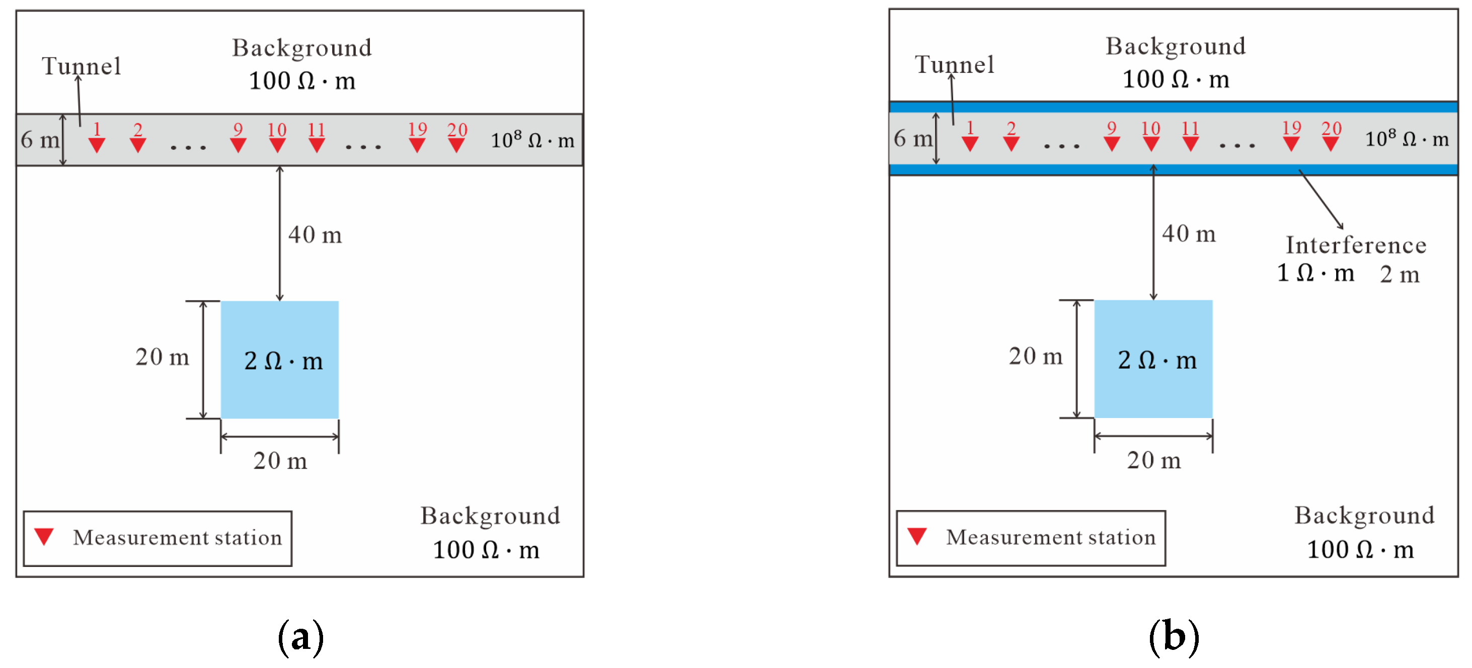
Figure 1. Synthetic models for analyzing the effect of interference on the inversion interpretation: (a) without interference; (b) with interference.
Minerals 14 00802 g001
Figure 2. Inversion results under the uniform background model as the initial model: comparison between the cases with and without interference (resistivity profiles are shown for the anomaly region only). (a) Data fitting curves without interference (Station 1, Station 5, and Station 10). (b) Resistivity profiles of the inversion in the absence of interference. (c) Data fitting curves under the influence of interference (Station 1, Station 5, and Station 10). (d) Resistivity profiles of the inversion under the influence of interference.
Minerals 14 00802 g002aMinerals 14 00802 g002b
Figure 3. Inversion results after using the correction factor method. (a) Data fitting curves obtained by inversion after correction (Station 1, Station 5, and Station 10). (b) Inversion result for corrected data.
Minerals 14 00802 g003
Figure 4. Inversion results after time-shift correction. (a) Data fitting curves of predicted and observed data after time-shift correction (Station 1, Station 5, and Station 10). (b) Inversion result for time-shift corrected data.
Minerals 14 00802 g004
Figure 5. Inversion results with interference added as a known factor to the initial model. (a) Data fitting curves for Station 1, Station 5, and Station 10. (b) Resistivity profile.
Minerals 14 00802 g005
Figure 6. Assuming the interference is unknown, the data from Station 1 are used for 1D inversion to obtain the effective resistivity model of the interference. This effective model is then mapped to 2D and used as the initial model for 2D inversion: (a) 1D inversion result from using Station 1 data; (b) 2D resistivity profile obtained by mapping the 1D inversion result; (c) 2D inversion result; and (d) data fitting curves for Station 1, Station 5, and Station 10.
Minerals 14 00802 g006
Figure 7. Underground mining tunnel and the geological changes around it.
Minerals 14 00802 g007
Figure 8. Interference survey in the mine tunnel. (a) The locations of measurement stations and the distribution of interferences in the tunnel. (b) Interference responses obtained from different measurement stations.
Minerals 14 00802 g008
Figure 9. Field data acquisition: (a) vertical view for the distribution of tunnels in the working space, and the distribution of TEM measurement stations in the tunnels; (b) field data collected in the mine tunnel.
Minerals 14 00802 g009aMinerals 14 00802 g009b
Figure 10. Numerical simulation of model parameter settings for the SCM. (a) Tunnel and interference distribution and resistivity settings. (b) The profile of the discretized resistivity model at x = 0 (The maximum boundary of the model is 3 km, and only the tunnel area is shown here).
Minerals 14 00802 g010
Figure 11. Correction of actual data: (a) simulated interference response and actual measurement response; (b) response after correction.
Minerals 14 00802 g011
Figure 12. Inversion result for field data without correction.
Minerals 14 00802 g012
Figure 13. Inversion results after correction: (a) inversion result for data corrected using the SCM; (b) inversion result for data corrected using the MCM.
Minerals 14 00802 g013
Figure 14. PICM-based inversion results: (a) 2D inversion result using the PICM alone; (b) 2D inversion result based on the MCM and PICM.
Minerals 14 00802 g014
Disclaimer/Publisher’s Note: The statements, opinions and data contained in all publications are solely those of the individual author(s) and contributor(s) and not of MDPI and/or the editor(s). MDPI and/or the editor(s) disclaim responsibility for any injury to people or property resulting from any ideas, methods, instructions or products referred to in the content.