An Alternative Method of Obtaining the Particle Size Distribution of Soils by Electrical Conductivity

Abstract

This study proposes a new method to determine the particle size distribution (PSD) of soils by considering the electrical conductivity (EC) technique. A new EC probe was designed with a transparent thermoplastic, commonly known as acrylic, and brass electrodes. At first, the EC of a soil–water homogeneous suspension was calculated at different densities to obtain a calibration curve of each tested soil sample. During the PSD analysis, as the particles started to settle down in the basement due to gravity, the EC was measured at different time intervals, and the corresponding EC values were then matched with the calibrated EC values at different densities. The proposed method considered the conventional Stokes’ law to determine the diameter of soil particles and the general percentage of passing mathematical expression to obtain the final PSD curve of each soil. The PSD analysis by the EC approach was later validated with that of hydrometer and laser diffraction methods, and in general, good agreements were obtained for identical soil samples at different classifications of soil particles such as clay, silt, and sand. Finally, reproducibility tests were also conducted and the new EC probe overperformed the hydrometer method in terms of both accuracy and precision. The finding from this study aimed to propose an alternative to determine the PSD of soils by using the EC technique with a high level of accuracy and efficiency.

1. Introduction

Particle size distribution (PSD) is a fundamental property of sediments and soils [1]. In general, the dynamic situations of transport and testimony of the constituent particles of rocks are usually determined by their PSD. The size distribution is an essential property for analysing the behaviour of granular material under any applied fluid or gravitational forces. A conventional PSD analysis involves the determination of the mass fractions of clay, silt, and sand [2,3]. These mass fractions can be presented either as a histogram or a cumulative plot [4]. In most of the PSD analyses, soil particles are considered to be spheres among other solid bodies, and only a sphere has a single characteristic linear dimension. Irregularly shaped particles may have different properties from which various distinctive linear dimensions can be acquired. The different properties include a particle’s projected area, volume, settling velocity, and length, and the size of the pathway through which the particle will pass [5].

PSD can be determined by both classical and modern techniques. The classical techniques generally include sieving and sedimentation. Two traditional sedimentation techniques, namely the hydrometer and pipette methods, are considerably affordable in cost and user-friendly [6,7,8]. However, the combination of sieving and a hydrometer is the most popular one (ASTM D422-63) [9]. Meanwhile, the modern trend in PSD analysis involves expensive and automated devices like laser diffraction [10,11], SediGraph [12,13], and dynamic image analysis (DIA) [14,15]. The traditional sedimentation-based techniques have been criticised for producing inconsistent results for particles < 1 µm in diameter due to the existence of Brownian motion and its influence on the rate of sedimentation [10,11]. In addition, the majority of the classical sedimentation-based techniques are time-consuming. A standard PSD analysis using a hydrometer may take up to 24 h to finalise. Classical methods also suffer from the disadvantage of creating possible disruption during the settlement of the particles. It is a well-known fact that the pipette and hydrometer techniques require operators to interrupt particles’ settlement. To solve most of the drawbacks of the classical methods, SediGraph and laser diffraction (LD) have gained popularity recently, where it is possible to complete a PSD analysis within just 5 to 20 min. However, SediGraph has been reported to provide erroneous results for soil particles with high absorption rates [16,17]. The device is established based on the theoretical assumption of the absorption homogeneity for all particles. This leads to a plethora of pitfalls as some soil particles with iron have been found to have high absorption rates, and therefore, the final PSD outcome will not be completely accurate [17]. Meanwhile, the LD technique is attributed to have excellent reproducibility in terms of both natural and laboratory-based soil samples. The process has been a major development in determining PSD; however, the LD approach fairly underestimates values of soil parameters, particularly in clay content, and overestimates the silt fraction [7,15,16]. It was observed that a pipette fraction < 2 μm corresponded to <8 μm for laser diffraction, which is one of the major technical disadvantages of the LD method [17,18,19]. Furthermore, the pipette, LD and SediGraph methods require highly skilled operators to finalise the calculation. In the last decade, more alternatives were sought for PSD determination, focusing on both accuracy and robustness. Integral suspension pressure (ISP) is one of the major developments that considered the chronological change in pressure measured with precise accuracy at a certain depth within the soil–water suspension to obtain PSD [20,21]. One of the primary advantages of the ISP method is the automation with no technical supervision during the process, which may also take up to 24 h [21]. Although the device is user-friendly, the standard analysis time could still be considered a lengthy process. Furthermore, the principle of the device is highly based on empirical statistical analysis, and the inventors reported the existence of stochastic errors in the mathematical analysis. The operators are also required to use the manufacturer-owned software to analyse the data in most of the delicate equipment, such as the LD and ISP methods. A comprehensive literature review of the existing PSD techniques with inherent advantages and disadvantages can be found in some of the published works [4,16,22,23]. However, based on the brief discussion above, it can be stated that finding an alternative method may still be required to accelerate the whole process by achieving improved accuracy concurrently.

Although there have been numerous attempts to find alternative methods of PSD analysis of soils, a method based on electrical resistivity or conductivity has not been considered yet. Since electrical conductivity is a function of soil mineralogy [24,25,26,27] and each soil type exhibits unique electrical conductivity, it could be another option for PSD analysis. In general sedimentation theory, soil particles fall freely due to gravity, and thus the variation in the density could be recorded. Hydrometers directly provide the overall density of the suspension, which varies with time due to the free fall of soil particles’ sedimentation. From the suspension’s density, the density of the solid is determined. With the density of the solid, the percentage of passing of soil particles corresponding to the measured diameter is calculated. As the particles start to fall freely, the presence of soil particles will be different at certain depths. Therefore, the electrical conductivity will be different in different timescales at the same location within a container or a beaker (standard beaker for sedimentation-based PSD analysis). Considering those fundamentals of sedimentation theory, it is possible to establish the correlation between the density and electrical conductivity of soils to obtain the PSD of clay soils within a shorter timescale.

The purpose of this study was to propose and explore an alternative technique to determine the PSD of soils by electrical conductivity measurements. The method was based on conventional sedimentation theory based on Stokes’ law. The newly developed EC probe recorded the changes in electrical conductivity of a homogeneous suspension as a function of density. Although the final experimental programme was conducted in a similar environment as a hydrometer or pipette, the sedimentation process remained uninterrupted. The PSD curve was obtained within 2 h from the new EC probe with great accuracy and precision as well as reproducibility. The obtained results were also validated with those of hydrometer and LD methods. Overall, the high accuracy provided compelling evidence to determine the PSD of soils through electrical conductivity.

2. Materials

2.1. Properties of Soils

The testing materials comprised soil samples, a dispersion agent, and the device to analyse PSD. The samples consisted of both natural soils and laboratory-suited clay-rich soils from industries. Dermosol, chromosol, and vertosol are named as per the Australian Soil Classification. The properties were obtained from the respective suppliers.

Kaolin and bentonite were from the laboratory-based category, whereas three other natural soils, namely chromosol, vertosol, and dermosol, were collected from different locations in Australia [24,26]. The relevant geotechnical properties of laboratory-based and natural soils are mentioned in

Table 1. Properties of tested clay soils of this study [4,24].

Properties	Kaolin	Bentonite	Dermosol	Chromosol	Vertosol
Liquid Limit (%)	74	504	59	58	49
Plastic Limit (%)	32	53	29	27	28
Specific gravity (Gs)	2.58	2.68	2.6	2.59	2.68
pH in water (28%–40% solid)	7	9.5	5.17	5.5	7.1
Cation Exchange Capacity (meq/100 g)	0.075	80	2.9	4.5	20

. The natural soils were collected within the 0–25 cm depth of the ground. Those three samples underwent chemical pre-treatment procedures following the standard demonstrated by ASTM D422-63 [9] and other published documents and laboratory manuals [28,29,30]. Along with the present approach, two other PSD analyses were conducted from conventional (hydrometer) and modern (laser diffraction) techniques for each sample. The results were considered as parts of the accuracy assessment as well as validation of the present approach.

2.2. Dispersion Agent

As Stokes’ law is influential in sedimentation analysis, the individual soil particles must be dispersed to ensure PSD accuracy. However, the finer grains of soil carry charges on their surface, and therefore, there lies a chance of forming flocs. As a consequence, instead of considering the diameter of the individual grain, the grain diameter obtained will be equal to the flocs’ diameter, which will lead to erroneous outcomes. Therefore, in sedimentation analysis, dispersion agents are added. In other words, the dispersion agent ensures proper separation or dispersion of discrete particles of soil, especially from the silt-to-clay range.

A small quantity of soluble chemical is added before the commencement of any sedimentation test, generally in the form of a certain amount of a prepared solution. In most of the experiments, sodium hexametaphosphate (also commercially known as Calgon) is considered to be one of the most appropriate and convenient dispersants [30,31]. However, the choice of dispersion agent solely depends on the type of soils considered for the test. The properties of Calgon, as provided by the supplier, have been presented in

Table 2. Properties of dispersion agent provided by the supplier.

Type of Properties	Information
Chemical formula	Na6O18P6
Molecular weight	611.77
Appearance	White crystals
Density (g/cm3)	2.484
pH in water	8.2

.

It is recommended that a fresh solution containing Calgon should be prepared each month or fortnightly. In the present experiment, the solution was prepared just before the commencement of the experimental tests. The present study considered 2 g of Calgon in 1 L suspension by following Head [30].

2.3. Hydrometer Approach for Validation

Both the pre-treatment and PSD analysis were conducted by following ASTM D63 [9]. The present EC approach was also developed based on the sedimentation theory based on which the hydrometer technique was established. Therefore, it was essential to validate the outcome from the EC approach with the standard hydrometer. A hydrometer is an instrument that is considered to determine the specific gravity of any liquid solution. The specific gravity of a soil suspension depends on the particle size and therefore, a hydrometer can be used to obtain the PSD of a specific soil sample. The calibration and test procedure of a hydrometer to determine the PSD of a soil can be found in detail in the literature [28], and this standard method was followed in the present study to validate the outcome of the EC of an identical sample. The standard long-stem hydrometer was used in the present study to prepare the validation dataset.

2.4. Laser Diffraction Technique for Validation

It was important to validate the outcome from the present EC approach with one of the modern devices. Therefore, the PSDs of the tested soil samples were also obtained through LD for validation. A Malvern Mastersizer 2000 Laser Diffraction particle size analyser (Malvern Panalytical Ltd., Malvern, UK) was considered to meet this objective. The readings were taken at room temperature. The pump speed and stirring speed were set at 2000 rpm and 800 rpm, respectively. The ultrasonic level was set at 100%. The PSD analysis was conducted based on the Mie theory and the outcome was recorded through the software provided by the manufacturer by four to five repeated measurements on each aliquot using a 30 s measurement time. The particle absorption index was set at 0.01, whereas the refractive index (RI) was 1.52. The RI of the distilled water was 1.33. Each analysis took 15 min to complete, including the data collection.

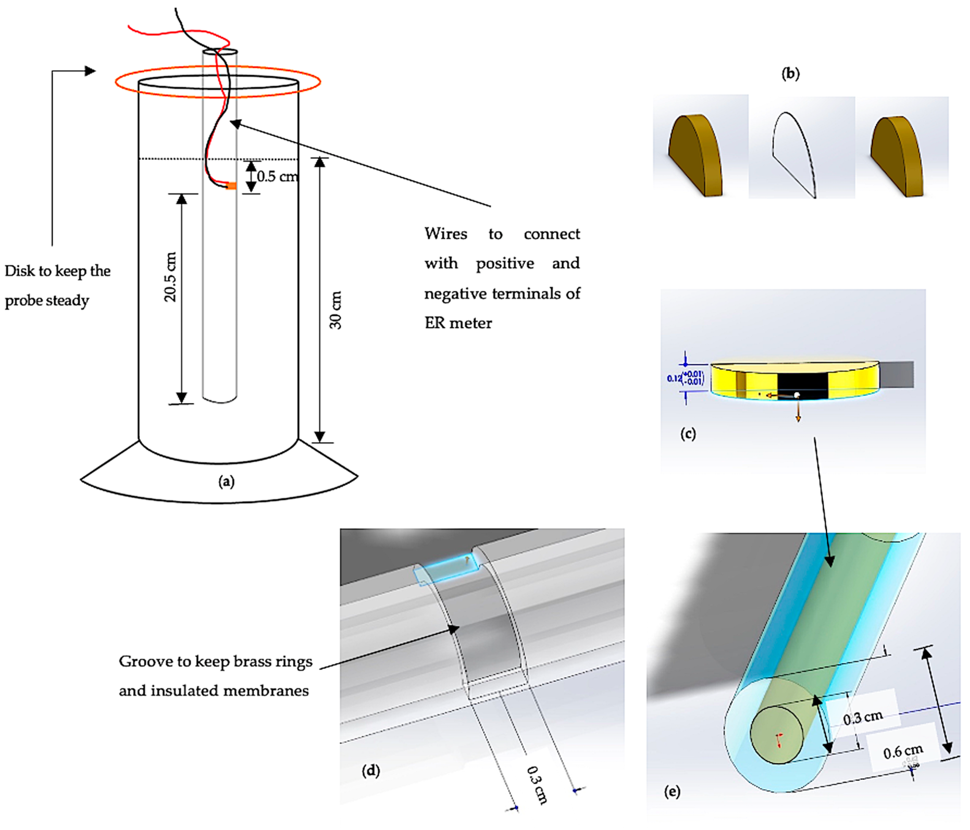
2.5. Newly Developed Electrical Conductivity Probe

In this experiment, the probe was constructed with a 50 cm clear acrylic tube containing one slot for the electrodes. The probe was customised with a Tormach CNC machine. The standard sedimentation beaker was used for the new approach, which is also used for the conventional PSD tests with a hydrometer and pipette. An acrylic circular disk, slightly bigger than the diameter of the cylinder, was placed on top of the beaker with a hole at the centre for the tube to go through. The hole was created in such a way so that the EC probe could be passed through and remained firm in its position to avoid slipping through completely within the soil–water suspension during the test. The schematic setup of the probe is shown in Figure 1a, where the placement of brass electrodes can be seen. There were two brass electrodes with identical shapes and designs, separated with a 0.1 mm laser transparency film to create insulation between the pair of electrodes, as shown in order in Figure 1b. The insulation was intended to avoid short circuits within the system. Each brass electrode had a half-ring shape with 0.12 cm thickness, as shown in Figure 1c. Therefore, the width of the groove was kept at 0.30 cm (Figure 1d) to accommodate two 0.12 cm brass rings (total 0.24 cm). The electrodes had small grooves on the top to connect the wires. The wires were passed through the top of the tube to connect with the resistivity meter. Then, the electrodes with an insulating membrane in the middle were affixed together and placed into the slot sequentially (as shown in Figure 1b) to complete the setup. The tube was then passed through the cylindrical disk to merge into the soil–water suspension. The tube’s inner and outer diameter were 0.6 cm and 0.8 cm, respectively (Figure 1e).

The electrical resistivity (ER)-measuring meter was connected with 2 wires to complete a circuit. As mentioned earlier, the new EC probe has two electrodes (positive and negative) in the slot. The two wires soldered with the brass rings were connected to two nodes of the resistivity meter. To ensure accurate reading, the meter was calibrated with three different chemical solutions with known electrical conductivity values within the laboratory environment. The solutions were provided by the manufacturers of the ER meter. From the ER readings, the conversion to EC was conducted immediately.

3. Methods

3.1. Theory and Mathematical Formulation

Sedimentation refers to the settling of particles under the effect of gravitational or centrifugal forces. Devices based on gravitational sedimentation measure the velocity of settling particles due to the gravitational forces acting on the particles, against the buoyancy of the fluid, as well as other drag forces against the setting of the particles. The mathematical relationship is expressed by Stokes’ law, which is valid only for particles settling under terminal velocity and non-turbulent flow. The terminal velocity (v) can be expressed as the following [28]:

$$\mathrm{v}={\displaystyle \frac{{\mathrm{d}}^2\left({\mathrm{G}}_{\mathrm{s}}-{\mathsf{\rho }}_{\mathrm{L}}\right)\mathrm{g}}{18\mathsf{\mu }}}$$

(1)

Here, d is the particle diameter (mm), g is the acceleration due to the gravity (m/s²), $\mathsf{\mu }$ is the fluid viscosity (Ns/m²), and ${\mathrm{G}}_{\mathrm{s}}$ and ${\mathsf{\rho }}_{\mathrm{L}}$ are the specific gravity of soils and fluid density (g/cm³), respectively.

From Equation (1), the diameter of soil particles passing at a specific time in a column of height h can be written as [28]

$$\mathrm{d}=\sqrt{{\displaystyle \frac{18\mathsf{\mu }\mathrm{h}}{\mathrm{g}\left({\mathrm{G}}_{\mathrm{s}}-{\mathsf{\rho }}_{\mathrm{L}}\right)\mathrm{t}}}}$$

(2)

Here, v = h/t was substituted to define a particle that falls a distance of h (cm) in time t (s). Fundamentally, the velocity of particles depends on their position in the suspension as well as the size (diameter) of the particles. In addition, due to increased sensitivity, it is important that there is a significant difference between the particle density and suspension density.

The diameter of the particle, d, can be calculated from Stokes’ law as described in Equation (2), and the passing of soil particles is calculated from the following equation [29]:

$$\mathrm{N}=\left({\displaystyle \frac{{\mathrm{G}}_{\mathrm{s}}}{{\mathrm{G}}_{\mathrm{s}}-1}}\right){\displaystyle \frac{{\mathsf{\rho }}_{\mathrm{s}}-{\mathsf{\rho }}_{\mathrm{f}}}{{\mathrm{M}}_{\mathrm{s}}}}\times 100$$

(3)

where ${\mathsf{\rho }}_{\mathrm{s}}$ is the density of the solid (g/cm³), ${\mathrm{M}}_{\mathrm{s}}$ is the mass of the soil (g), and ${\mathrm{G}}_{\mathrm{s}}=({\displaystyle \frac{\mathrm{u}\mathrm{n}\mathrm{i}\mathrm{t} \mathrm{w}\mathrm{e}\mathrm{i}\mathrm{g}\mathrm{h}\mathrm{t} \mathrm{o}\mathrm{f} \mathrm{s}\mathrm{o}\mathrm{i}\mathrm{l}}{\mathrm{u}\mathrm{n}\mathrm{i}\mathrm{t} \mathrm{w}\mathrm{e}\mathrm{i}\mathrm{g}\mathrm{h}\mathrm{t} \mathrm{o}\mathrm{f} \mathrm{w}\mathrm{a}\mathrm{t}\mathrm{e}\mathrm{r}}}$) is the specific gravity, which is unitless.

3.2. EC Approach with Sedimentation

The proposed approach is similar to the sedimentation theory, but instead of following the hydrometer or pipette method, the electrical conductivity of the suspension was included in the experiment. At the beginning of sedimentation, the soil particles are homogeneously dispersed throughout the suspension, and therefore, the concentration of soil particles of different diameters should remain consistent at different depths. During the process of sedimentation, fluid–soil particle interactions will take place that can lead to the formation of a diffuse double layer (DDL) [26]. Soil particles have distinctive characteristics. A high-swelling clayey soil will most likely show rapid changes in conductivity due to the development of DDLs. These changes can be monitored by observing the changes in the EC values at different timescales. The electrical properties of the DDL will be controlled by the salinity due to the dispersion agent, as distilled water will have no impact on the DDL’s development [26]. The rapid changes in EC can be cross-matched with the calibrated density values. The changes in EC will depend on the type of sample. Soil with a larger DDL (such as bentonite) will exhibit more variations in the EC values, and density can be obtained each time with those changes even if the differences are not significant.

After a certain period, only unsettled particles remain at certain depths. In other words, all particles larger than a certain particular size (d in Equation (2)) will be settled below that certain depth. The present approach utilises this theory of sedimentation and relies on Equations (2) and (3) to find the final PSD, similar to a hydrometer or a pipette method. However, the proposed approach was dependent on the electrical conductivity of soils. It required calibration by finding the electrical conductivity of the soil–water suspension at different densities. Later, those calibrated datasets were used to predict the density of the solid from the electrical conductivity values.

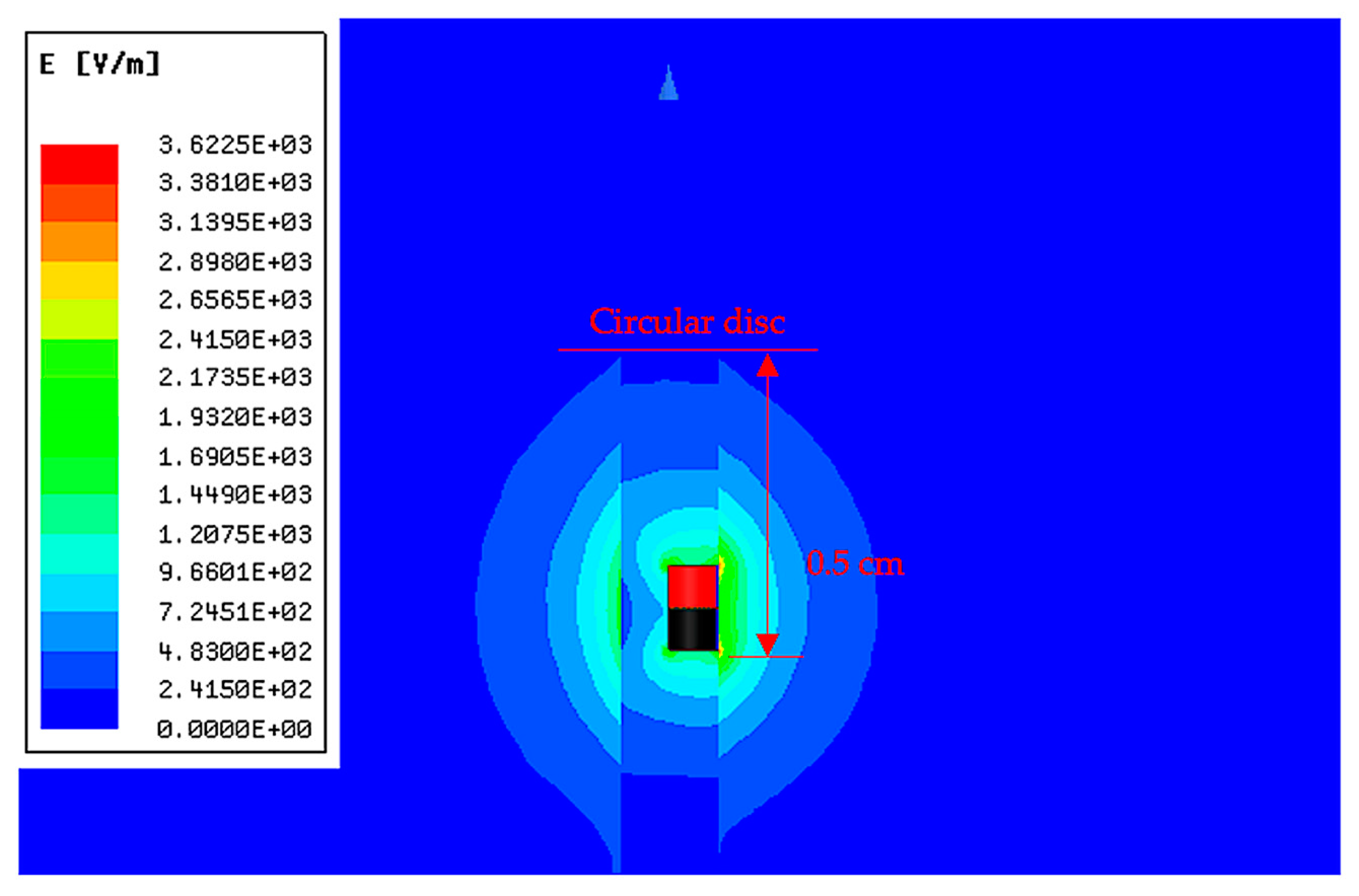
3.3. Effective Distance Measurement

The two electrodes, separated with a thin film layer, were modelled in ASNYS Maxwell to determine the appropriate distance to install the electrodes (Figure 2). The electrodes were made from brass, while the thin film layer was made of insulation material. The modelled tube was made from acrylic. However, the optimum distance to install the electrodes was also determined. The purpose was three-fold. First of all, the electrodes were targeted to be placed in proximity to the water level. It was important to test whether the electric field overlapped with anything above the water level. Secondly, the aim was to obtain the full intensity of the electric field within the suspension to maximise the space within the beaker. Finally, the electrodes were placed on one side of the tube. It was important to test the homogeneity of the electric field distribution to demonstrate the uniformity of the approach. This means that the PSD outcomes would be identical if the electrodes of the tube were placed left-sided instead of right-sided. The next task was to obtain evidence of such claims.

The equation used to calculate the electric field is written as the following [32,33]:

$$\mathrm{E}=-\nabla \mathsf{\varphi }=-\left({\displaystyle \frac{𝜕\mathsf{\varphi }}{𝜕\mathrm{x}}}\overrightarrow{\mathrm{i}}+{\displaystyle \frac{𝜕\mathsf{\varphi }}{𝜕\mathrm{y}}}\overrightarrow{\mathrm{j}}+{\displaystyle \frac{𝜕\mathsf{\varphi }}{𝜕\mathrm{z}}}\overrightarrow{\mathrm{k}}\right)$$

(4)

where $\mathsf{\varphi }$ is the voltage vector potential and $\overrightarrow{\mathrm{i}},\overrightarrow{\mathrm{j},}\overrightarrow{\mathrm{k}}$ are the unit vectors at x, y, and z axes, respectively.

The boundary conditions were put on the faces of the calculation area with restrictions on the voltage. At V = 0, the lines of the electric field will be zero on the face of the calculation area. In such a case, the calculation area should be sufficiently large compared to the model, and therefore, it will not affect the result. It can be seen from the results that the calculation area is large enough because the value of the electric field comes to zero before touching the boundary face (Figure 3).

To find the effective distance, an arbitrary 5 V was applied through ANSYS Maxwell. An identical dimension of the acrylic tube was considered including the insulation, as shown in Figure 2. After several iterations, the results showed that the optimum distance was found to be 0.5 cm from the water surface, as shown in Figure 3. In addition, homogeneity of the suspension was also ensured, and therefore, the outcomes were not impacted despite placing the electrodes facing one side (right-sided) only. It was not pragmatic to consider a whole circular ring as it would have increased the complexity of the manufacturing and would have required a more rigid material. This process would have increased the manufacturing cost.

3.4. Experimental Programmes

The experimental programmes were divided into three parts. The first part required pre-treatment to prepare the soil samples as per the standard ASTM D422-63 [9]. After the pre-treatment, the samples were calibrated at different amounts of tested soil sample (nearest to 0.1 g). In the final part of the experiment, the PSD was calculated, and necessary comparisons were made with other established approaches.

3.4.1. Pre-Treatment Steps

The following briefly describes the steps followed for the soil pre-treatment [4,9]:

i.

About 25 g of oven-dried soil was weighed accurately with a balance and transferred to a glass beaker. The glass beaker was washed properly with distilled water before the commencement of the test.

ii.

The soil was then subject to chemical pre-treatments, which were performed in two stages, namely organic material removal and calcium compound elimination. First, the soil was pre-treated with a hydrogen peroxide (H₂O₂) solution (20 volume) to remove the organic matter at a rate of 1 mL/g of the sample (Figure A1a). Then, the mixture was kept steady to allow oxidation to take place. Hydrogen peroxide caused oxidation of the organic matter, and a small amount of gas was generated (Figure A1b). The mixture was kept steady for 10–15 min until no more bubbles appeared. After this, the mixture was sieved with a 75 μm sieve. If less concentrated hydrogen peroxide is used, the mixture will require heating with a Bunsen burner, with a temperature not exceeding 600 °C.

iii.

The soil remaining from step (ii) was transferred to another clean glass beaker. To remove the calcium compounds, 0.2 M hydrochloric acid (HCl) was added to the soil at a rate of 1 mL/g soil (Figure A1c). When the reaction ended, the mixture was filtered again. The filtrate was washed properly with distilled water until it was completely free from the acid. The damp soil was transferred to an evaporating dish. Both the damp and filtrated soils were oven-dried overnight, and their mass was recorded.

iv.

The next day, the oven-dried pre-treated soils were transferred to a clean beaker.

v.

The mixture was then stirred vigorously for 30 min using a mechanical stirrer. The contents of the mixture were then transferred to the cup of a mechanical stirrer. The cup should not be filled to more than ¾, as the turbulence created by the rotating blade may cause the mixture to spill out of the cup. Stirring time may vary based on the soil properties. For more clayey soils, the stirring period should be increased.

vi.

The suspension was washed through the 75 μm sieve again using distilled water. The portion which passed through the sieve was taken for the experiment. The specimen was washed in a cylindrical 1000 mL glass jar and adequate water was added to make 1000 mL of suspension. After this, the whole suspension was mixed properly to ensure homogeneity.

vii.

The cylindrical glass jar was then kept inside a water tank which had a temperature-controlling motor. The whole experiment was conducted inside the water tank so that the temperature did not affect the conductivity value.

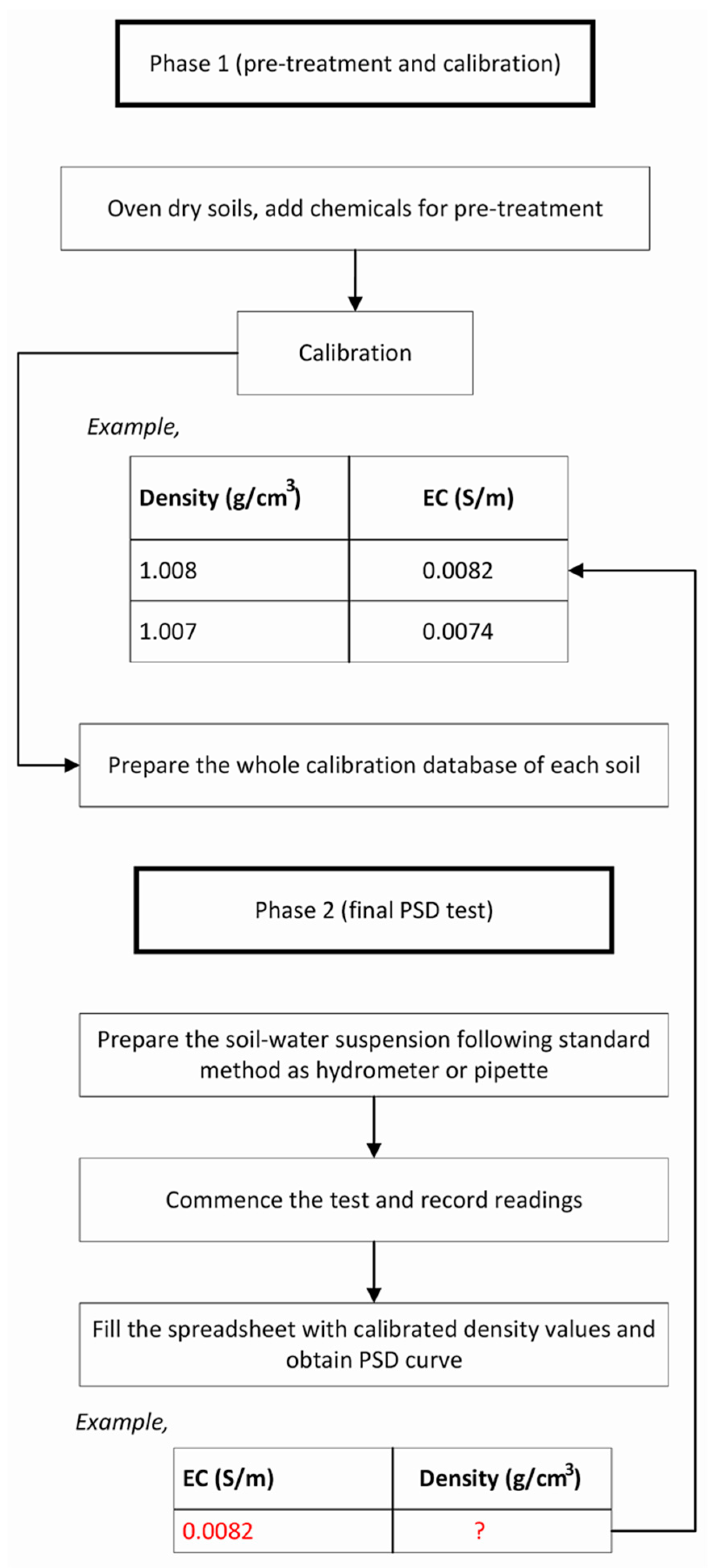
3.4.2. Calibration by EC for PSD Analysis

In a particular soil–water suspension settling under gravity, the concentration of the suspended particles stays constant inside the beaker. This means that the density will be different at different time intervals. This concept led to the idea that the suspension of different densities can be calibrated with electrical resistivity or conductivity values. For example, the density of the water is approximately 1 g/cm³. The total density will increase if 25 g of soil is added to create a suspension. The amount of dispersing agents should be deducted while recording the density values. The correction to exclude the dispersion agent was also tested separately with the water–Calgon solution.

All the PSD techniques that are available require calibration to some extent. It was seen that the requirement of the calibration technique in this research gave satisfactory results for all the samples. The repetition of the technique provided more confidence in building calibration data. It should be mentioned that the amount of dispersing agent was kept the same for the actual test as well.

For each type of sample, calibrations can be performed in two different ways, namely (i) straight calibration at different densities and (ii) three-point calibration and interpolations or, simply, regression. Technique (i) could be time-consuming but more accurate. A standard PSD analysis by conventional methods is conducted with 25 g of soil. Therefore, calibrations were conducted at different densities of soils, ranging from 1.001 g/cm³ to 1.025 g/cm³. At different densities of suspension, different values of electrical resistivity were recorded with the ER meter and converted into EC values. Each test was repeated at least thrice, and only 0.1%–0.5% discrepancies were noticed. Meanwhile, the three-point calibration requires taking the EC readings at the lowest, mid, and highest density ranges. After that, the rest of the EC values can be predicted by linear or polynomial interpolations, based on the EC behaviours of the soil samples. Sample examples are shown in Figure 4a (kaolin) and Figure 4b (vertosol).

3.4.3. Correction of EC Values in Calibration

The correction of the dispersing agent’s density was required since all of the tested suspensions had a fixed amount included for both the calibration and the final experiment, to find the PSD. That is why one dispersing agent’s density correction test was conducted before starting the calibration.

Readings were taken carefully using an ER meter, and the whole test was conducted within two hours, but it can vary based on the sample type. As the electrical interactions among one type of soil particles are not similar to another soil type, individual calibration for each soil sample was mandatory to obtain precise data during the actual experiment. The overall process is presented with a flowchart in Figure 5 to provide a clear view, including sample examples of interpreting the EC values to obtain the density of soils. If the EC of a particular interval did not match the calibrated values, the closest calibrated value with less than a 2% difference was selected for that specific reading. To ensure accuracy in the calibration, the data from the three-point test were also used for the assessment.

3.4.4. Steps of EC Measurement

After the completion of the pre-treatment and calibration, the final EC measurement for PSD analysis was conducted as follows:

I.

A 1 L suspension with 25 g of soil was prepared as described before. To ensure homogeneity, the palm of a hand on the open end of the sedimentation beaker was placed to turn it upside down and back repeatedly a few times.

II.

A stopwatch was started to record the time. The first reading was taken at t = 1 min

III.

The recording of EC changes continued by considering a 5 min interval. Not all the changes will be important for the PSD analysis. However, the operator can skip a measured point if the difference is marginal.

IV.

The experiment ends at t = 120 min. The measured EC values on the spreadsheet are then compared with the calibrated density values. If any specific EC value is not matched with the calibrated density values, then either the closest value in the calibration or the equation through the 3-point calibration can be used.

V.

The final PSD curve is then obtained. The experimental time can be extended if only 50% of passing soil particles are obtained. However, this situation will be unlikely since the sedimentation process was not interrupted.

VI.

After the completion of each test, the beaker was removed from the water tank and cleaned properly with de-ionised water. Before starting the experiment with the next sample, all of the tools were cleaned and dried out appropriately to avoid contamination in the samples.

4. Results

The obtained PSD outcomes were recorded on a standard log scale as per the standard. After that, each PSD curve obtained from the EC approach was compared with the results of the hydrometer and LD. Finally, a reproducibility assessment was also conducted at least three times, and each time, the EC approach demonstrated fewer inconsistencies in the results than a hydrometer.

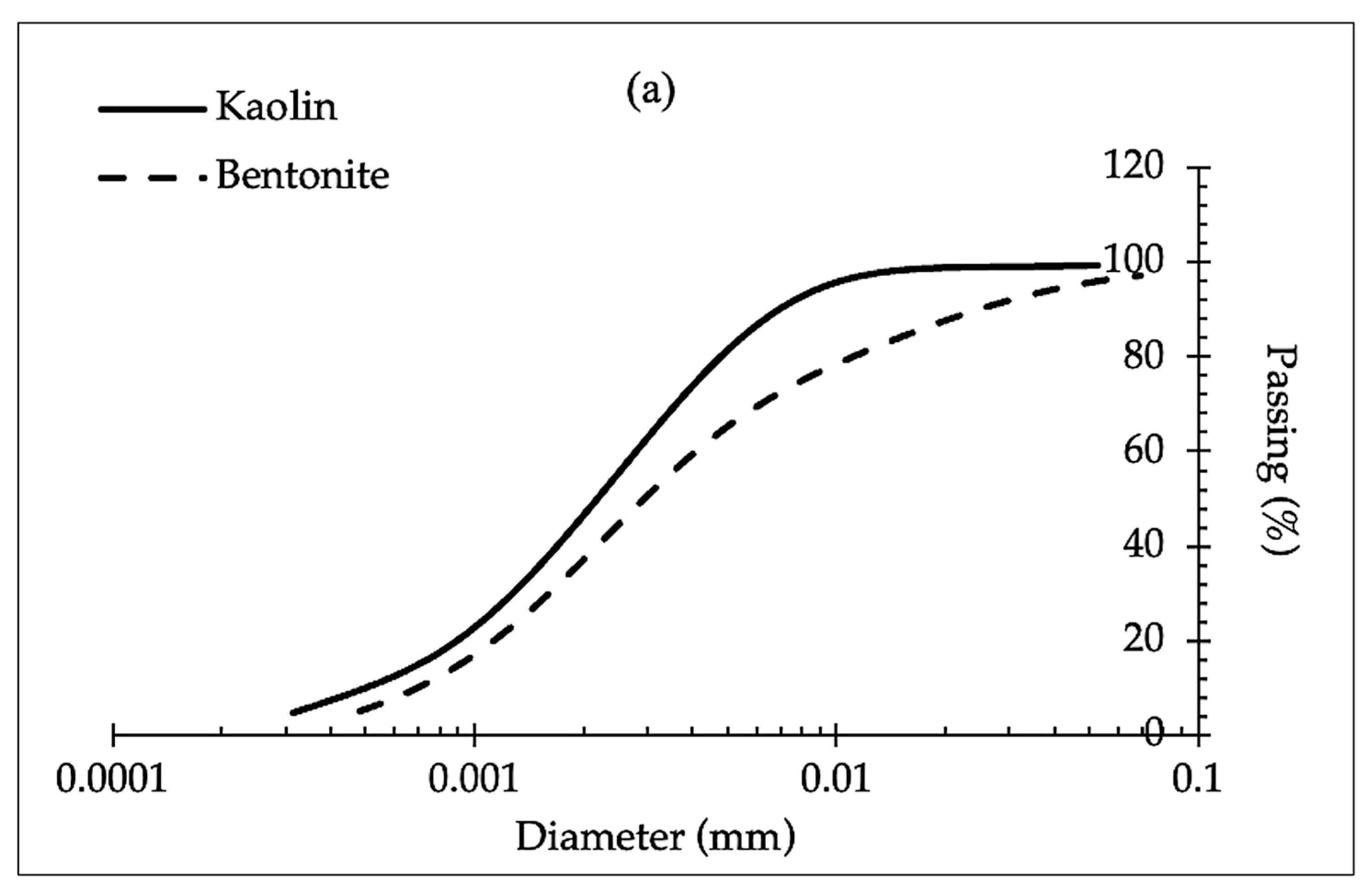
4.1. Particle Size Distribution by Electrical Conductivity

The PSD results are presented in Figure 6 for both laboratory-based soils (Figure 6a) and natural soils (Figure 6b). All the results in Figure 6 were obtained from the present EC approach within 2 h. It could be seen that the new probe was able to cover a wide range of particle diameters. To secure more confidence in the approach, the results were subject to accuracy and reproducibility analyses. In the following section, the PSD curves, obtained from the present approach, are subject to a discussion on accuracy and reproducibility. It has been mentioned earlier that the PSD of each soil sample was also found using a hydrometer and the laser diffraction technique.

4.2. Accuracy Assessment

Figure 7 depicts that the present approach was able to produce the PSD curves of the corresponding soil samples, which were in good agreement with the existing methods. Some minor discrepancies could be observed in terms of the results obtained from the hydrometer and laser diffraction. It has been mentioned that LD underestimates PSD analysis compared to that of the pipette method for identical samples. Figure 7a suggests that almost all methods exhibited similar results. Kaolin is an inert clay and is easy to use for PSD analysis. Therefore, more validations were conducted for other soils as well to investigate the variations.

Figure 7b–e represent the PSD results of bentonite, vertosol, dermosol, and chromosol, respectively. Significant discrepancies can be observed between the outcomes from the hydrometer and LD in Figure 7b–e. In most of the cases, the hydrometer overestimated the results in both clay and silt fractions, with more than 15% discrepancies observed for chromosol in Figure 7d. The EC approach overestimated some points at the clay fraction (Figure 7b,c), as well as sometimes underestimating at the silt fraction (Figure 7b–d).

A quantitative assessment is presented in

Table 3. Cross-validation of EC approach with laser diffraction and hydrometer through quantitative assessment of different types of soil particles. Blank R² and LCCC values indicate a lack of measured data for a statistical comparison.

Sample	Benchmark	Particle Type	R2	LCCC
Kaolin	Laser diffraction	Clay	0.97	0.86
		Silt	0.99	0.97
		Sand	0.99	0.97
	Hydrometer	Clay	0.80	0.96
		Silt	0.87	0.85
		Sand	0.99	0.97
Bentonite	Laser diffraction	Clay	0.97	0.73
		Silt	0.97	0.81
		Sand	0.99	0.94
	Hydrometer	Clay	0.99	0.95
		Silt	0.98	0.98
		Sand	0.98	0.82
Vertosol	Laser diffraction	Clay	-	-
		Silt	0.99	0.99
		Sand	0.98	0.88
	Hydrometer	Clay	-	-
		Silt	-	-
		Sand	0.98	0.98
Dermosol	Laser diffraction	Clay	-	-
		Silt	0.94	0.86
		Sand	0.97	0.93
	Hydrometer	Clay	-	-
		Silt	-	-
		Sand	0.98	0.97
Chromosol	Laser diffraction	Clay	-	-
		Silt	-	-
		Sand	0.99	0.98
	Hydrometer	Clay	-	-
		Silt	-	-
		Sand	0.94	0.81

, describing the accuracy by considering the laser diffraction and hydrometer methods as benchmarks each time. The purpose was to compare the outcomes obtained from the present EC approach with different types of soil particles with both the laser and hydrometer techniques. All the tested samples were considered for cross-validation. In terms of accuracy assessment metrics, the coefficient of determination (R²) and Lin’s concordance correlation coefficient (LCCC) were recorded. Based on the soil particle diameters, clay (<0.002 mm), silt (0.002 mm to 0.05 mm), and sand (0.05 mm to 2 mm) were categorised. Both kaolin and bentonite had all three types of particles available in the PSD analysis. It can be observed from Table 3 that 0.97 ≤ R² ≤0.99 and 0.80 ≤ R² ≤0.99 were obtained for kaolin and bentonite, respectively, by comparing with the outcomes from the hydrometer and laser diffraction. Meanwhile, 0.96 ≤ LCCC ≤ 0.97 was achieved for kaolin and 0.76 ≤ LCCC ≤ 0.97 was obtained for bentonite overall by combining both validation benchmarks. The accuracy was comparatively greater in the prediction of sand particles than clay and silt for both kaolin and bentonite as they settled quicker than the rest due to their bigger particle dimension (0.05 mm to 2 mm). Clay particles are the smallest in this cohort (<0.002 mm), and the settling time was more than that of silt and sand. Therefore, laser diffraction and the hydrometer may have different percentages of passing. The EC approach showed more accuracy in the clay fraction with the comparison of the hydrometer for both kaolin and bentonite in terms of accuracy and precision through LCCC. The values of LCCC by comparing EC outcomes with the hydrometer at the clay fraction were found to be 0.96 and 0.95, respectively, compared to 0.86 and 0.73 with the laser diffraction approach. The overall prediction was found to be satisfactory and accurate at the silt and sand fractions with both laser diffraction and the hydrometer (kaolin and bentonite).

A similar comparison by using natural soils (vertosol, dermosol, and chromosol) was not feasible due to having no sufficient measured data in the clay range through either a hydrometer or the present EC approach. Natural soils were coarser than kaolin and bentonite. Therefore, there were not enough measured points for the accuracy assessment. It should be mentioned here that at least three points were considered for R² calculation, and four points were required for an accurate LCCC value. This also explains some of the missing values in Table 3 in terms of the cross-validation accuracy of clay fractions of natural soils (vertosol) and, in some cases, both clay and silt (dermosol and chromosol). In fact, Figure 7 also shows such PSD curves for the natural soils, where there are not enough measured points at the clay fraction of the natural soils (Figure 7c–e). However, the PSD curves covered a wider range in terms of laboratory soils like kaolin (Figure 7a) and bentonite (Figure 7b). Nevertheless, the prediction accuracy of the natural soils’ PSD was still acceptable with 0.94 ≤ R² ≤ 0.99, 0.86 ≤ LCCC ≤ 0.99 (EC comparison with laser diffraction) and 0.94 ≤ R² ≤ 0.98, 0.81 ≤ LCCC ≤ 0.98 (EC comparison with a hydrometer).

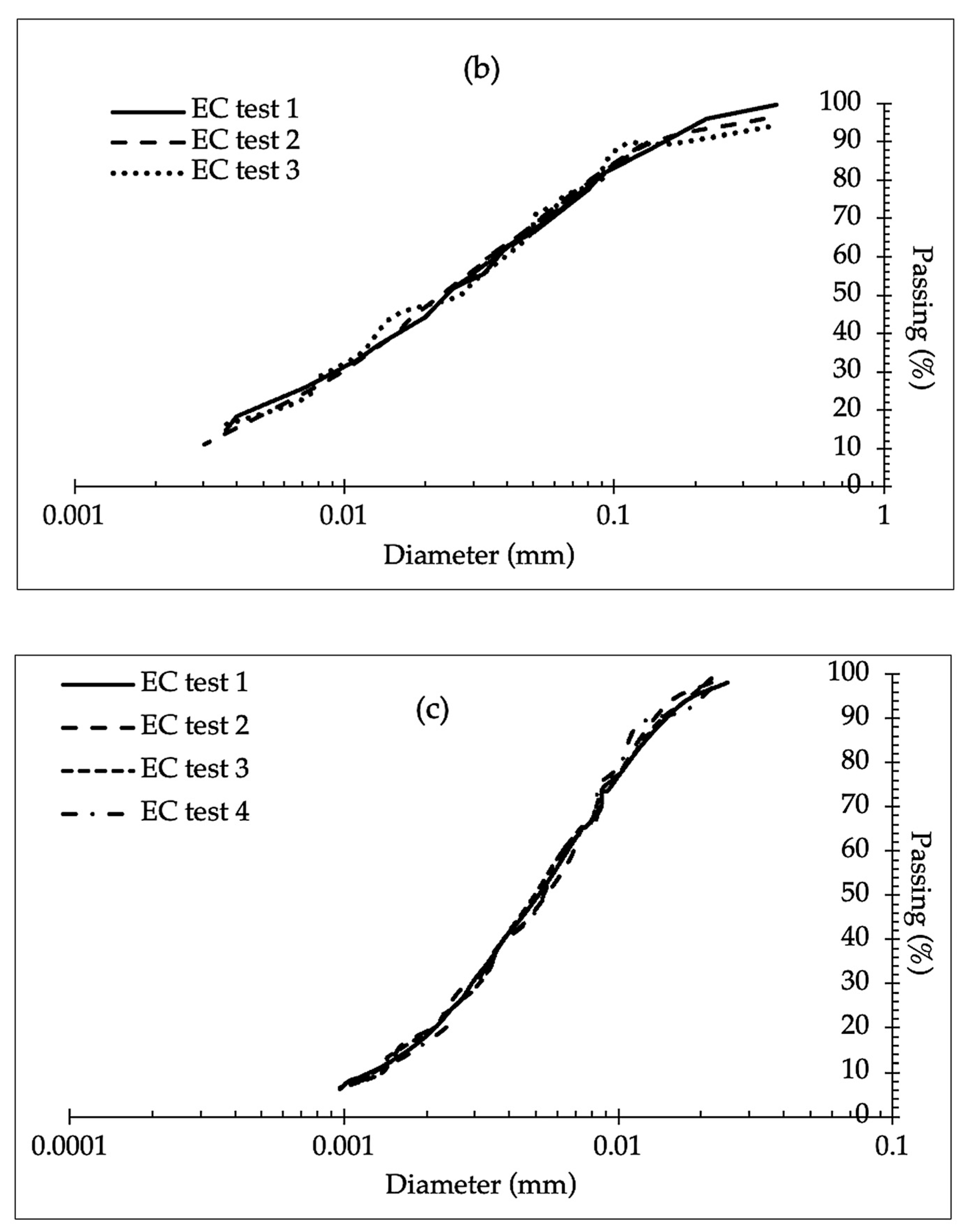
4.3. Reproducibility of Results

The reproducibility of the present approach was tested as well, considering the results from laser diffraction as the benchmark data. It is evident from Figure 8a that the results obtained from the hydrometer test had approximately 10%–12% differences for dermosol in comparison with the laser diffraction outcome, whereas there were around 1%–2% differences in the repeated results of the present test, as presented in Figure 8b (dermosol) and Figure 8c (kaolin). Unlike the hydrometer, the EC probe was always submerged in the suspension, which caused almost zero disruption to the particles’ settlements, and hence, the results were almost identical. In addition, the calibration was conducted based on the EC–density relation based on a mathematical formula rather than recording the density based on the scales on a hydrometer by manual observation.

The frequency of the reproducibility test varied based on the availability of the sample. The reproducibility of the hydrometer results was tested at least twice. The EC approach was tested between three and five times. Each repetition test was conducted with the same equipment. Therefore, the results provide compelling evidence that the present approach can provide more accurate results than a hydrometer within 2 h. It was tested for all the soils considered in this study, and similar differences were observed.

5. Discussion

5.1. Advantages of Present Approach

The conventional methods like using a hydrometer and pipette are user-friendly and do not require high technical skills. However, hydrometers significantly interrupt the particles’ settlement each time a reading is recorded. Pipettes do the same, and it is fair to say that more caution needs to be taken in each sampling to avoid creating bubbles. Pipette sampling needs to be taken in one go, and the pressure on the rubber suction bulb needs to be slow and steady. Both techniques require at least 24 h to finalise the experiment. In an industrial setup, a 24 h waiting period could be a major challenge as it limits the analysis time, and no appropriate scientific step can be taken to accelerate the approach. Compared to the temporal disadvantage of the hydrometer and pipette, the EC technique can produce PSD curves of both laboratory and natural soils within 2 h. Furthermore, the present EC technique does not require the operator to collect samples or disturb the settlement of the soil particles. The EC recording activities were performed outside the chamber, and therefore, the internal settlement process is not interrupted. It also eliminates the requirement to hire a highly skilled operator to obtain the PSD of each soil. The EC approach uses the same formulae as hydrometers and pipettes, and therefore, no complicated mathematical interpretation is required either. It can be observed from Figure 7 and Figure 8 that the quicker analysis of the PSD of soil does not compromise the quality of the outcome.

On the other hand, SediGraph and LD devices are expensive and delicate, and only highly skilled operators with knowledge of particles’ optical properties, such as the refractive index, and in-house software are able to use them. Furthermore, most users have reported high maintenance costs (in terms of both expenses and time). The EC probe only requires washing with de-ionised water before starting another experiment with a different soil type. There is no requirement to use any descaling chemical either for maintenance. The dispersion agent and other chemicals used for the pre-treatment of clay soils are the standard procedures for all conventional methods and are inexpensive. While pre-treatment can be avoided for the SediGraph and LD methods, the calibration of optical properties along with sensitivity testing is still required for each soil type. The present EC approach was still able to compete with LD methods in terms of both accuracy and reproducibility, as shown in Figure 7 and Figure 8.

5.2. Insensitivity to Types of Soils

The soil samples considered in this study had distinctive geotechnical properties and availability. Most of the natural soils have liquid limits within 20%–100%, with the majority within 40% to 60%. As per Table 1, dermosol, vertosol, and chromosol all had liquid limits within this range (59%, 49%, and 58%, respectively). Kaolin was a laboratory-based clay and had a liquid limit of 74%. The present EC technique was able to produce accurate PSD curves for those soils. Bentonite had a liquid limit of 504%. Bentonite itself has a complex physico-chemical structure. Montmorillonite-rich bentonite has high plasticity and swelling capacity. Therefore, it is always a challenge to work with bentonite–water suspensions. The results from Figure 6a and Figure 7b are compelling evidence that the present EC approach was not only applicable for low-plasticity soils but also for a high-swelling clay-rich soil like bentonite.

Meanwhile, the three natural soils considered in this study had different chemical properties, which are good representatives of similar types of soils. For example, chromosol is a sodic soil and has a pH = 4.6, and dermosol has a pH = 4.3. However, vertosol had a pH = 7.1, which is almost double the pH of chromosol and dermosol. Therefore, the present EC approach was able to predict accurate PSD of soils with high and low pH. Based on the aforementioned discussions on the variations in the physico-chemical properties, the selection of five different soils is justified for validation.

5.3. Analysis of the Efficiency of the Approach

Figure 7 is an example of the present EC probe’s accuracy in terms of existing methods. While both the LD and hydrometer methods were considered as benchmarks for the validations, some discrepancies were observed. As per Figure 7, some of the obtained results from the EC approach were overestimations within the clay range. This discrepancy could be attributed to the earlier discussion that LD typically underestimates the clay content. Therefore, the overestimation from the EC approach could have been accurate, considering that LD might have underestimated within the clay range. This was also demonstrated through cross-validation, as shown in Table 3, as the prediction accuracy and precision of the present EC approach at the clay fraction was comparatively lower with LD compared to that with the hydrometer.

However, in terms of reproducibility, the EC approach outperformed hydrometer tests, as compared in Figure 8. Two repeated tests were conducted for both the hydrometer and EC approach within the same environment with all the soils, but only the outcomes with vertosol and kaolin soil were presented. The inaccurate reproducibility of hydrometer results has been reported in the past [34], and as per Figure 8a, a good amount of discrepancies in terms of repeated tests were observed. On the other hand, the EC probe was able to produce identical results, as shown in Figure 8b. Considering that soil is a heterogenic material, it is practically impossible to obtain identical results each time, regardless of the type of steps taken for the treatment [35]. However, the ability to reproduce the results with less deviation should still be achievable, and it will provide a more compelling reason to trust a specific method for PSD analysis. Despite the soil heterogeneity and the overestimation and underestimation issue with LD, the present EC approach was also able to demonstrate excellent reproducibility with almost identical results for the same soil.

5.4. Factors Affecting the Accuracy

Soil is a complex material, and each soil exhibits certain characteristics. Despite the long waiting period for the hydrometer and pipette, those methods are still in practise due to their easier operational procedure and moderate accuracy. Murad et al. [36] attempted to automate the hydrometer approach, but the shortcomings regarding the inaccurate estimation of soil particles’ diameter will still exist. Although the automation process will reduce manual labour, the method does not improve hydrometer readings and the settling time is still close to 8 h. Therefore, the EC method could still be a better alternative as it has the capability of producing more accurate results with better reproducibility within just 2 h. However, no specific method is completely accurate. As per Figure 7a, the EC probe displayed the most overestimated value of the passing diameter of 0.02273 mm compared to that of LD and the hydrometer. In addition, the PSD curve of vertosol soil in Figure 6b is not entirely smooth compared to that of laboratory-based clay-rich soils like kaolin and bentonite in Figure 6a. However, none of those shortcomings were major disadvantages, which the following aims to explain.

There were a few factors that might have affected the accuracy and efficacy of the EC approach. The accuracy assessment was carried out by making a comparison with sedimentation and LD methods. However, those are based on different conceptual theories. Researchers were found to be divided in supporting the methods. The information on LD accuracy as well as overestimating silt and underestimating clay fractions was discussed earlier. However, some published works also reported that even the pipette method considers a constant bulk density value of soil as 2.65 g/cm³, which cannot be ideal for all types of soils due to the presence of coarser contents such as sand [37]. In addition, the reason for inaccurate PSD prediction by sedimentation could be attributed to the assumption of the spherical soil particles. Non-spherical particles settle comparatively slower than spherical ones [16]. As per the results obtained, it can be said that, considering that the hydrometer and LD methods are still in practise, the present EC approach could also be a reliable option to consider in the future. This is one of the reasons for validating the obtained outcomes from the existing method with those aforementioned techniques.

The calibration of density against EC values was the most important step of this newly introduced technique. Inaccurate calibration will lead to errors in the final PSD analysis. While the process involved calibrating at different densities through careful weight measurement of each sample, the method might not have been completely accurate. Each time a specific amount of sample was mixed for calibration, the reading was not taken immediately as the suspension required a few seconds to be steady. This waiting period might have affected the homogeneity of the suspension, and therefore, the calibration could have been 2%–3% less accurate. Furthermore, the ER meter sometimes does not provide stable results and that leads to mixing the sample again and waiting for it to be steady to repeat the reading for calibration. However, this problem was rarely faced as the steadiness of the EC probe and the soil–water suspension was always checked before the final reading. Nevertheless, the experimental procedure was still convenient to implement and did not require specific knowledge of any complicated properties such as the refraction index in SediGraph or tedious sample collection, as with a pipette.

5.5. Limitations and Future Recommendations

While the manufacturing of the EC tool cuts and placement of the groove was carried out by the Tormach CNC machine, the assembly was conducted manually, including soldering, creating the path for wire extensions, and affixing electrodes with epoxy. Although the EC probe was able to produce accurate results, the assembly technique is likely to vary from person to person. Extra care should be given while affixing the electrodes with epoxy as improper mixing will negatively impact the functionality underwater. In addition, the drying out of epoxy may take more than 24 h depending on the indoor environment and type of adhesive. Before the commencement of the experimental programme, it should be formally tested whether the sealing of electrodes into the acrylic groove was properly carried out. All activities involving assembly were tedious, yet a one-off task. As long as accuracy was the fundamental objective, the EC probe was still able to produce more satisfactory results than the existing methods, regardless of the inconvenience of the assembly tasks. The present EC probe was made with industrial-grade acrylic that could withstand most of the inorganic chemicals such as diluted acids, alkalis, and oil. While the PSD analysis does not require submerging the device into chemical-induced water solutions, it is recommended to select the acrylic to manufacture the probe based on the ability to withstand harsh pressure, temperature, and chemicals to prolong the lifespan of each probe.

The EC probe can be further improved by automating data collection by attaching the probe to a datalogger. The ER meter can be replaced with appropriate sensors to make the process fully automated, but this might increase the overall cost of the experiment and introduce the requirement of a skilled operator to calibrate and maintain those sensors. However, the maintenance cost would still be less than laser diffraction or SediGraph. Nevertheless, the present EC probe still produced highly accurate results without the need for those requirements. Therefore, automation can be a good addition if implemented, but not obligatory. Finally, the present study considered five different types of soils with diverse geotechnical properties. Due to a lack of sufficient samples, it was not feasible to test the EC probe with more samples. A validation with a larger dataset (approximately 200 samples) would provide more confidence in the accuracy of the approach. To validate such a bigger dataset, the PSD of each sample from a hydrometer and laser diffraction will also be required. This is currently under investigation, and further outcomes will be reported in the future.

6. Conclusions

The current study proposes a new method to determine the particle size distribution (PSD) of soils using the electrical conductivity (EC) technique and soil mineralogy. The new tool considers the conventional sedimentation theory, Stokes’ law, and formulae for the percentage of passing to provide the final PSD curve of each soil. Five different soils with diverse properties ranging from high to low swelling capability, pH, clay content, CEC, and organic materials were considered to test the accuracy of the probe. The EC probe considered the EC of soils at different densities for calibration, and later, density values were cross-matched with the calibrated EC values during the final PSD analysis. The matched EC values at different time intervals provided density values, and that information was put together inside the typical PSD formulae to obtain the final curve. The complete PSD outcome was achieved within 2 h, and the obtained results were validated against conventional techniques such as a hydrometer and a modern laser diffraction (LD) analysis tool. The present EC probe was able to display a high level of accuracy, including excellent reproducibility. The limitation of the LD tool in underestimating clay content and overestimating the silt fraction for some soils was also experienced by the EC probe. Furthermore, the obtained results from the EC probe were found to be more accurate than those of conventional hydrometers. The outcomes from this study suggested that the EC of soils could be efficiently interpreted with density to obtain PSD analysis. Finally, based on the manufacturing costs, quicker assessment time, and user-friendliness of the EC probe, it could be a great alternative in the future to determine the PSD of any soil sample. In terms of future research, more emphasis has to be given to automating the process to avoid dependency on manual operators.

References

1. Liu, D.; O’Sullivan, C.; Carraro, J.A.H. The Influence of Particle Size Distribution on the Stress Distribution in Granular Materials. Géotechnique 2023, 73, 250–264. [Google Scholar] [CrossRef]
2. Ma, S.; Song, Y.; Liu, J.; Kang, X.; Yue, Z.Q. Extended Wet Sieving Method for Determination of Complete Particle Size Distribution of General Soils. J. Rock Mech. Geotech. Eng. 2024, 16, 242–257. [Google Scholar] [CrossRef]
3. Yang, Y.; Jaber, M.; Michot, L.J.; Rigaud, B.; Walter, P.; Laporte, L.; Zhang, K.; Liu, Q. Analysis of the Microstructure and Morphology of Disordered Kaolinite Based on the Particle Size Distribution. Appl. Clay Sci. 2023, 232, 106801. [Google Scholar] [CrossRef]
4. Hasan, M.F. Electrical Conductivity of Saturated Fine-Grained Soils: Modelling and Soil Classification Applications. Ph.D. Thesis, La Trobe, Melbourne, Australia, 2020. Available online: https://opal.latrobe.edu.au/articles/thesis/Electrical_Conductivity_of_Saturated_Fine-Grained_Soils_Modelling_and_Soil_Classification_Applications/14227487 (accessed on 21 May 2024).
5. Wei, Y.; Wu, X.; Cai, C. Splash Erosion of Clay–Sand Mixtures and Its Relationship with Soil Physical Properties: The Effects of Particle Size Distribution on Soil Structure. Catena 2015, 135, 254–262. [Google Scholar] [CrossRef]
6. Bouyoucos, G.J. Hydrometer Method Improved for Making Particle Size Analyses of Soils. Agron. J. 1962, 54, 464–465. [Google Scholar] [CrossRef]
7. Gee, G.W.; Bauder, J.W. Particle Size Analysis by Hydrometer: A Simplified Method for Routine Textural Analysis and a Sensitivity Test of Measurement Parameters. Soil Sc. Soc. Am. J. 1979, 43, 1004–1007. [Google Scholar] [CrossRef]
8. Beuselinck, L.; Govers, G.; Poesen, J.; Degraer, G.; Froyen, L. Grain-Size Analysis by Laser Diffractometry: Comparison with the Sieve-Pipette Method. Catena 1998, 32, 193–208. [Google Scholar] [CrossRef]
9. ASTM D422 63; Standard Test Method for Particle-Size Analysis of Soils. ASTM International: West Conshohocken, PA, USA, 2017.
10. Eshel, G.; Levy, G.J.; Mingelgrin, U.; Singer, M.J. Critical Evaluation of the Use of Laser Diffraction for Particle-Size Distribution Analysis. Soil Sci. Soc. Am. J. 2004, 68, 736–743. [Google Scholar]
11. Bittelli, M.; Pellegrini, S.; Olmi, R.; Andrenelli, M.C.; Simonetti, G.; Borrelli, E.; Morari, F. Experimental Evidence of Laser Diffraction Accuracy for Particle Size Analysis. Geoderma 2022, 409, 115627. [Google Scholar] [CrossRef]
12. Magno, M.C.; Venti, F.; Bergamin, L.; Gaglianone, G.; Pierfranceschi, G.; Romano, E. A Comparison between Laser Granulometer and Sedigraph in Grain Size Analysis of Marine Sediments. Measurement 2018, 128, 231–236. [Google Scholar] [CrossRef]
13. Milligan, T.G.; Law, B.A.; Zions, V.; Hill, P.S.; Hua, K.; McKindsey, C.W.; Lacoursière-Roussel, A. Reconciling Coulter Counter and Laser Diffraction Particle Size Analysis for Aquaculture Monitoring. Environ. Monit. Assess. 2024, 196, 672. [Google Scholar] [CrossRef] [PubMed]
14. Shang, Y.; Kaakinen, A.; Beets, C.J.; Prins, M.A. Aeolian silt transport processes as fingerprinted by dynamic image analysis of the grain size and shape characteristics of Chinese loess and Red Clay deposits. Sediment. Geol. 2018, 375, 36–48. [Google Scholar] [CrossRef]
15. Zheng, J.; Hryciw, R.D. Soil particle size and shape distributions by stereophotography and image analysis. Geotechn. Test. J. 2017, 40, 317–328. [Google Scholar] [CrossRef]
16. Jones, R.B. Rotational Diffusion of a Tracer Colloid Particle: I. Short Time Orientational Correlations. Phys. A Stat. Mech. Appl. 1988, 150, 339–356. [Google Scholar] [CrossRef]
17. Dapkunas, S.J.; Jillavenkatesa, A.; Lum, L.H. Particle Size Characterization. In NIST Recommended Practice Guide, SP 2001; NIST: Gaithersburg, MD, USA, 2001; pp. 960–961. [Google Scholar]
18. Sochan, A.; Bieganowski, A.; Bartmiński, P.; Ryżak, M.; Brzezińska, M.; Dębicki, R.; Stuczyński, T.; Polakowski, C. Use of the Laser Diffraction Method for Assessment of the Pipette Method. Soil Sci. Soc. Am. J. 2015, 79, 37–42. [Google Scholar] [CrossRef]
19. Taubner, H.; Roth, B.; Tippkötter, R. Determination of Soil Texture: Comparison of the Sedimentation Method and the Laser-diffraction Analysis. Z. Pflanzenernähr. Bodenk. 2009, 172, 161–171. [Google Scholar] [CrossRef]
20. Durner, W.; Iden, S.C.; Von Unold, G. The Integral Suspension Pressure Method (ISP) for Precise Particle-size Analysis by Gravitational Sedimentation. Water Res. Res. 2017, 53, 33–48. [Google Scholar] [CrossRef]
21. Zhang, X.; Warren, C.J.; Spiers, G.; Voroney, P. Comparison of the Integral Suspension Pressure (ISP) and the Hydrometer Methods for Soil Particle Size Analysis. Geoderma 2024, 442, 116792. [Google Scholar] [CrossRef]
22. Allen, T. Particle Size Measurement; Springer: Berlin/Heidelberg, Germany, 2013; Available online: https://books.google.com/books?hl=en&lr=&id=7dsFCAAAQBAJ&oi=fnd&pg=PR17&dq=Allen,+T.+(2013).+Particle+size+measurement.+Springer.&ots=SnhnPMps_i&sig=qm9TQ-2KfrtAkhjhOJ69vpCDt5o (accessed on 21 May 2024).
23. Messing, I.; Soriano, A.M.M.; Svensson, D.N.; Barron, J. Variability and Compatibility in Determining Soil Particle Size Distribution by Sieving, Sedimentation and Laser Diffraction Methods. Soil Tillage Res. 2024, 238, 105987. [Google Scholar] [CrossRef]
24. Hasan, M.F.; Abuel-Naga, H. Determining Liquid Limit and Plastic Limit of Clay Soils by Electrical Surface Conduction and Diffuse Double Layer Thickness. Minerals 2024, 14, 210. [Google Scholar] [CrossRef]
25. Choo, H.; Park, J.; Do, T.T.; Lee, C. Estimating the Electrical Conductivity of Clayey Soils with Varying Mineralogy Using the Index Properties of Soils. Appl. Clay Sci. 2022, 217, 106388. [Google Scholar] [CrossRef]
26. Hasan, M.F.; Abuel-Naga, H. Effect of Temperature and Water Salinity on Electrical Surface Conduction of Clay Particles. Minerals 2023, 13, 1110. [Google Scholar] [CrossRef]
27. Oh, T.-M.; Cho, G.-C.; Lee, C. Effect of Soil Mineralogy and Pore-Water Chemistry on the Electrical Resistivity of Saturated Soils. J. Geotech. Geoenviron. Eng. 2014, 140, 06014012. [Google Scholar] [CrossRef]
28. Day, P.R. Physical Basis of Particle Size Analysis by the Hydrometer Method. Soil Sci. 1950, 70, 363–374. [Google Scholar] [CrossRef]
29. Arora, K.R. Soil Mechanics and Foundation Engineering: In SI Units; Standard Publishers Distributors: New Delhi, India, 2000. [Google Scholar]
30. Head, K.H. Manual of Soil Laboratory Testing; Pentech Press: London, UK, 1980; Volume 1, Available online: http://www.whittlespublishing.com/userfiles/shop/errata/198.pdf (accessed on 21 May 2024).
31. Lucena, P.G.; Aquino, R.V.; Sousa, J.E.; Júnior, V.S.S.; Pacheco Filho, J.G.; Pereira, C.F. Mineral and Particle-Size Chemometric Classification Using Handheld near-Infrared Instruments for Soil in Northeast Brazil. Geoderm. Reg. 2024, 38, e00819. [Google Scholar] [CrossRef]
32. Feynman, R.P.; Leighton, R.B.; Sands, M.; Hafner, E.M. The Feynman Lectures on Physics; Vol. I. Am. J. Phys. 1965, 33, 750–752. [Google Scholar] [CrossRef]
33. Maxwell, J.C. VIII. A dynamical theory of the electromagnetic field. Phil. Trans. R. Soc. 1865, 155, 459–512. [Google Scholar]
34. Gee, G.W.; Bauder, J.W. Particle-Size Analysis. In SSSA Book Series; Klute, A., Ed.; Soil Science Society of America, American Society of Agronomy: Madison, WI, USA, 2018; pp. 383–411. [Google Scholar]
35. Polakowski, C.; Ryżak, M.; Sochan, A.; Beczek, M.; Mazur, R.; Bieganowski, A. Particle Size Distribution of Various Soil Materials Measured by Laser Diffraction—The Problem of Reproducibility. Minerals 2021, 11, 465. [Google Scholar] [CrossRef]
36. Murad, M.O.F.; Jones, E.J.; Minasny, B. Automated Soil Particle-size Analysis Using Time of Flight Distance Ranging Sensor. Soil Sci. Soc. Am. J. 2020, 84, 690–699. [Google Scholar] [CrossRef]
37. Polakowski, C.; Sochan, A.; Bieganowski, A.; Ryzak, M.; Foldenyi, R.; Toth, J. Influence of the Sand Particle Shape on Particle Size Distribution Measured by Laser Diffraction Method. Int. Agrophys. 2014, 28, 195–200. [Google Scholar] [CrossRef]
Figure 1. New PSD determination tool with EC approach: (a) schematic of the setup, (b) assembly of electrodes, (c) location for wire soldering to create the circuit, (d) the groove to put half-rings and insulated membrane, and (e) design of the tube.
Minerals 14 00804 g001
Figure 2. ANSYS design of the probe with insulations included.
Minerals 14 00804 g002
Figure 3. Effective distance observation from ANSYS Maxwell simulations.
Minerals 14 00804 g003
Figure 4. Comparison between calibration at different densities and regression based on the 3-point test for (a) kaolin and (b) vertosol.
Minerals 14 00804 g004
Figure 5. Flowchart of the PSD analysis through the present EC method.
Minerals 14 00804 g005
Figure 6. PSD curves from EC approach of soils: (a) laboratory-based and (b) natural.
Minerals 14 00804 g006aMinerals 14 00804 g006b
Figure 7. Comparisons of outcomes from EC approach with hydrometer and laser diffraction methods for (a) kaolin, (b) bentonite, (c) vertosol, (d) dermosol, and (e) chromosol.
Minerals 14 00804 g007aMinerals 14 00804 g007bMinerals 14 00804 g007c
Figure 8. Reproducibility of PSD tests by (a) hydrometer, (b) EC approach with dermosol (three repeats), and (c) EC approach with kaolin (four repeats).
Minerals 14 00804 g008aMinerals 14 00804 g008b