Dissolution Mechanisms and Surface Charge of Clay Mineral Nanoparticles: Insights from Kinetic Monte Carlo Simulations

Abstract

The widespread use of clay minerals and clays in environmental engineering, industry, medicine, and cosmetics largely stems from their adsorption properties and surface charge, as well as their ability to react with water. The dissolution and growth of minerals as a function of pH are closely related to acid–base reactions at their surface sites and their surface charge. The vivid tapestry of different types of surface sites across different types of clay minerals generates difficulties in experimental studies of structure–property relationships. The aim of this paper is to demonstrate how a mesoscale stochastic kinetic Monte Carlo (kMC) approach altogether with atomistic acid-base models and empirical data can be used for understanding the mechanisms of dissolution and surface charge behavior of clay minerals. The surface charge is modeled based on equilibrium equations for de/protonated site populations, which are defined by the pH and site-specific acidity constants (pK_as). Lowered activation energy barriers for these sites in de/protonated states introduce pH-dependent effects into the dissolution kinetics. The V-shaped curve observed in laboratory experiments is reproduced with the new kMC model. A generic rate law for clay mineral dissolution as a function of pH is derived from this study. Thus, the kMC approach can be used as a hypothesis-testing tool for the verification of acid–base models for clay and other minerals and their influence on the kinetics of mineral dissolution and growth.

1. Introduction

Clay minerals are extremely interesting materials for a variety of reasons. First, they are ubiquitous minerals in surface and subsurface geological environments, occurring in soils, sediments, water, and crystalline and sedimentary rock assemblages, as well as in the pore space of oil and gas reservoirs. Second, they are widely used materials in different industries and everyday life. Clay minerals serve as natural barriers for radionuclide entrapment [1,2,3], sorbents of toxic ions in natural environments [4,5,6] and the human body [7], important components of cosmetics, hair, and skincare products, building and road construction materials, dishware and pottery materials, and sculpting materials in the arts, in education, and in mental health therapies, as well as being used in many other useful and important applications. Finally, the large variety of clay mineral structures and compositions makes them an interesting and complex object of challenging research, where the fundamental properties of complex materials can be better understood and tested.

The number of studies and amount of published research on clay minerals are incredibly large; there are more than 30,000 publications available in English on the internet that are dedicated to applications of clay minerals [8]. The CLAYFF force field [9,10], dedicated to the molecular modeling of clay minerals and other layered materials, is one of the most cited and used force fields in applied mineralogy. Not surprisingly, studies of these widespread, useful, and tremendously complex materials have been the focus of substantial efforts from the scientific community for decades. The adsorption properties of clay minerals are one of the primary targets for environmental engineering studies, tackling issues of nuclear waste retention [1,3,11,12,13,14,15,16,17,18,19,20], water cleaning and purification [5,21,22,23], and the adsorption of toxic ions, e.g., chromium, zinc, arsenic, etc. [5,6,22,24,25,26,27,28,29,30,31], as well as organic pollutants [32,33].

Adsorption properties are essentially related to the charge of the mineral surface and the acid–base behavior of the surface sites at different pH conditions [34,35]. Clay minerals occur mostly in nano- and micro-particulate forms, where the grain edges of nanoparticles (NPs) play an important role in their reactive properties. Screw dislocations may also present and control the formation of nano- and micro-particles, as well as generating additional atomic steps [36,37] that are kinetically active during crystal growth and dissolution. The dissolution of clay mineral NPs may substantially alter their morphology, their surface structure, and the types of surface sites controlling the surface charge and adsorption. The dissolution process also decreases the mass and volume of nanoparticulate matter in rocks, which may change their porosity and permeability. Moreover, changes in pH might trigger the aggregation or disaggregation of particles, and may change their transport properties in pore space [34].

Understanding and studying the mechanistic relationships between clay’s mineral crystal structure, its chemical composition, the molecular structure of the clay–water interface, and its reactive and adsorption properties, as well as the kinetics of clay mineral dissolution and growth altogether, can be a very challenging task. The aim of this study is to put together a mechanistic picture of the clay mineral dissolution process and its surface charge behavior as a function of water acidity (pH). A special goal is to take into account molecular-scale processes and show how they affect material behavior at the microscopic scale, as well as how these processes are reflected in macroscopic experimental data. A previously developed kinetic Monte Carlo model for phyllosilicate dissolution [38] is used to construct models for muscovite and illite nanoparticle dissolution as a function of pH. The new model contains charge-dependent surface speciation, which enables the possibility of kinetic studies for pH-dependence. The reactions of deprotonation and protonation of surface sites are considered as ultrafast (femtosecond time scale) [39] in comparison to silicate bond hydrolysis reactions with high activation barriers [40,41,42,43,44,45]. This assumption allows us to combine equilibrium thermodynamics and kinetic approaches for reactions taking place at two very separate time scales. A similar approach was successfully used before for calcium carbonate, where we combined the equilibrium Grand Canonical Monte Carlo method for surface site speciation and the kinetic Monte Carlo method for dissolution kinetics as a function of the pH [46]. The new model for clay mineral nanoparticles represents a test study case for the possibility of implementation and usability of such models, rather than a fully developed and tested process simulator. The primary purpose of the present study is to develop and test a robust methodological approach for understanding the reactive behavior of clay minerals from atomistic to microscopic scales.

2. Methods

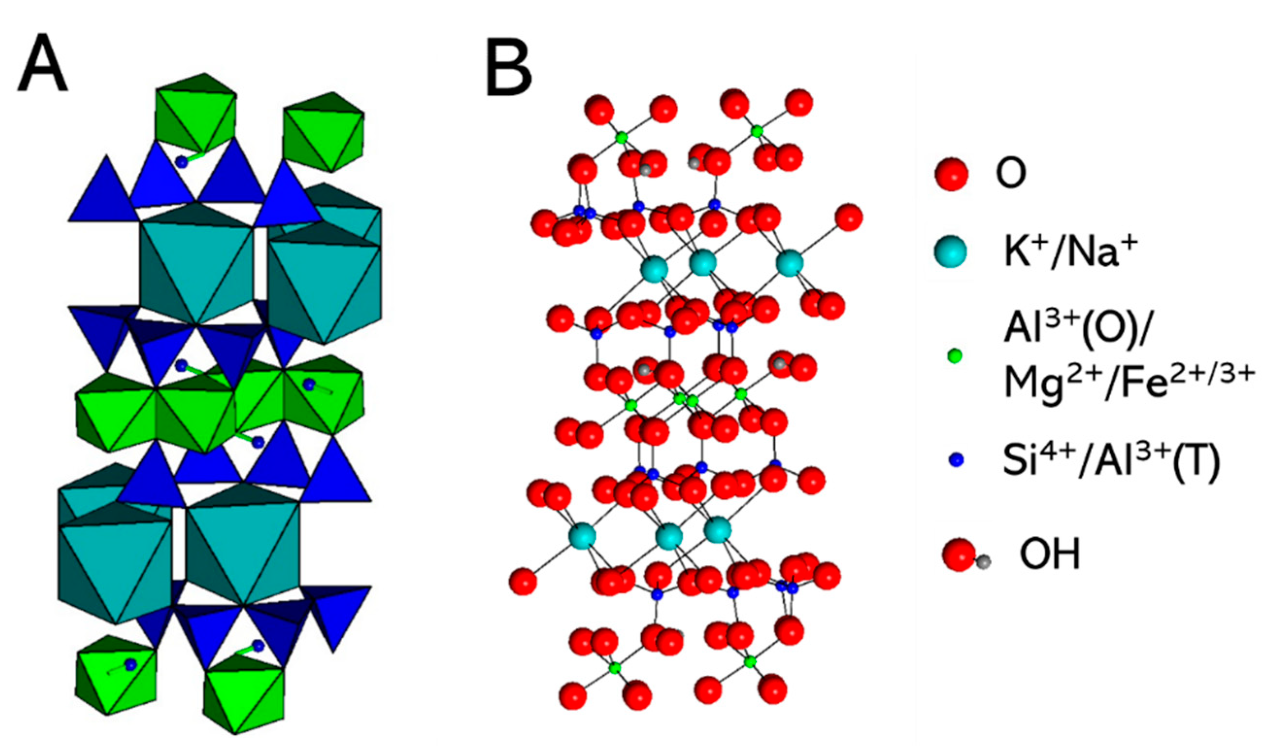
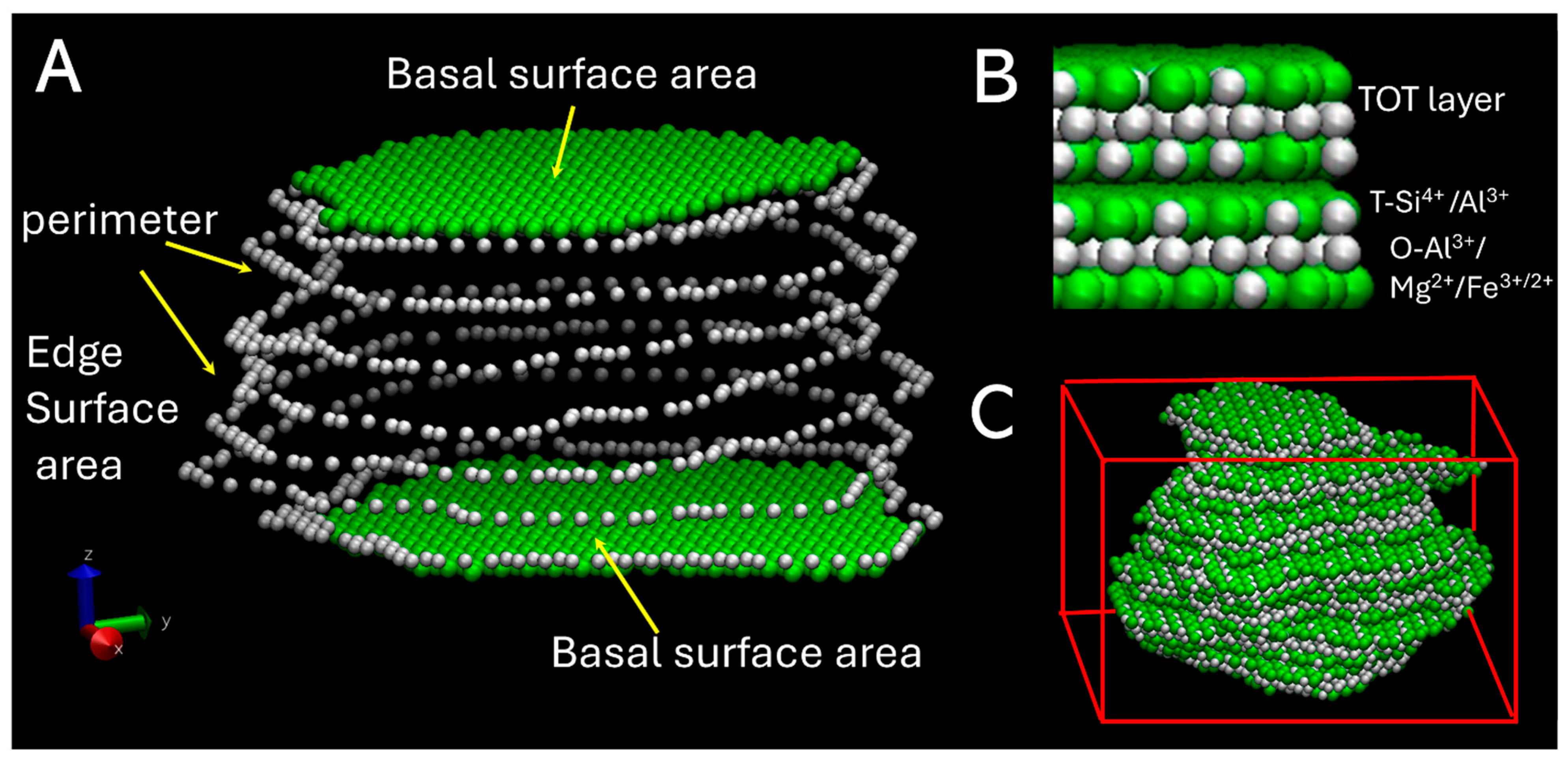
2.1. Simulated System

The muscovite 2M₁ polytype structure was used as a structural template for 2M₁ illite simulations (Figure 1). The unit formula for illite is thus a modified structural formula of muscovite, which can be represented as (Al_xFe_yMg_z)₂(AlSi₃)O₁₀[(OH₂),(H₂O)], without interlayer cations (K, etc.). The interlayer cations were ignored in the present study as they are weakly connected by ionic and Van der Waals forces in comparison to the strong covalent bonding of the aluminosilicate framework. We used the same unit cell parameters and source for fractional atomic coordinates [47] as in the previous KMC study of phyllosilicate dissolution [38]: $a=5.1918\mathrm{\AA },b=9.0153\mathrm{\AA }$, $c=20.0457$ Å, $\alpha =90°$, $\beta =95.735°$, γ = $90°$. Clay mineral nanoparticles were generated by translating a unit cell along crystallographic a, b, and c directions, with elongation along a direction according to a nanoparticle model of hexagonal and lath-shaped illite by Kuwahara [36,37]. There were two types of unit formulas considered in the present study: (I) “muscovite”: muscovite (AlSi₃) in the tetrahedral layer, and Al only in the octahedral layer; (II) “illite”: (Si_0.8875Al_0.1125) in the tetrahedral layer and (Al_0.6Fe_0.18Mg_0.22) in the octahedral layer corresponding to the illite composition used in the study by Köhler et al. [48]. Al atoms were randomly seeded into tetrahedral positions; Fe and Mg were randomly seeded into octahedral positions.

2.2. The Kinetic Monte Carlo Algorithm

The KMC model, algorithm, and in-house code were developed based on the previously published KMC model for phyllosilicate dissolution [38]. The probabilities for dissolution events were calculated by using the same approach as in the previous study, based on the number and types of bonds, as well as including second-order coordination spheres, and the steric factor for the OH group hindrance in octahedral layers. The principal difference between this model and the previous one is the incorporation of protonation and deprotonation reactions, construction of nanoparticles and incorporation of Mg and Fe into the octahedral layer. The time step is calculated as it was described by Voter [49]:

$$∆t=-{\displaystyle \frac{1}{v}}·{\displaystyle \frac{\mathrm{l}\mathrm{n}\left(rand\right)}{\sum _{i=1}^N{P}_i}}$$

(1)

where $v$ is the reaction attempt frequency, taken as a universal constant 10¹² Hz, which corresponds to the water vibration frequency and can be used to approximate the Arrhenius pre-factor [43], $P_i$ are individual probabilities of reactive events which are calculated as exponential functions of the energetic parameters ($∆E_i$), the number of bonds, first- and second-order coordination spheres, chemical types of bonds and their structural position (tetrahedral or octahedral). See more details in Kurganskaya and Luttge, 2013 [38]. The novelty of the present model is the incorporation of Mg²⁺ and Fe^2+/3+ into the octahedral layer. Therefore, nine new types of chemical bonds were considered, with the corresponding activation energy parameters per bond (see

Table 1. Energetic parameters used to calculate dissolution probabilities (this study) according to the model presented in Kurganskaya and Luttge, 2013 [38].

Type of Bond, i	∆Ei, kT Units	Type of Bond, i	∆Ei, kT Units
Si-Si	8.0	Si-Mg(O)	9.0
Si-Al(T)	6.0	Si-Fe(O)	10.0
Si-Al(O)	5.0	Al(T)-Mg(O)	7.0
Al(T)-Al(O)	5.0	Al(T)-Fe(O)	8.0
Al(O)-Al(O)	5.0	Al(O)-Mg(O)	6.0
OH-steric factor	1.0	Al(O)-Fe(O)	7.0
2nd order T-T	4.0	Mg(O)-Fe(O)	7.5
2nd order O-O	2.5	Mg(O)-Mg(O)	7.0
2nd order T-O	2.5	Fe(O)-Fe(O)	8.0
2nd order O-T	2.0

).

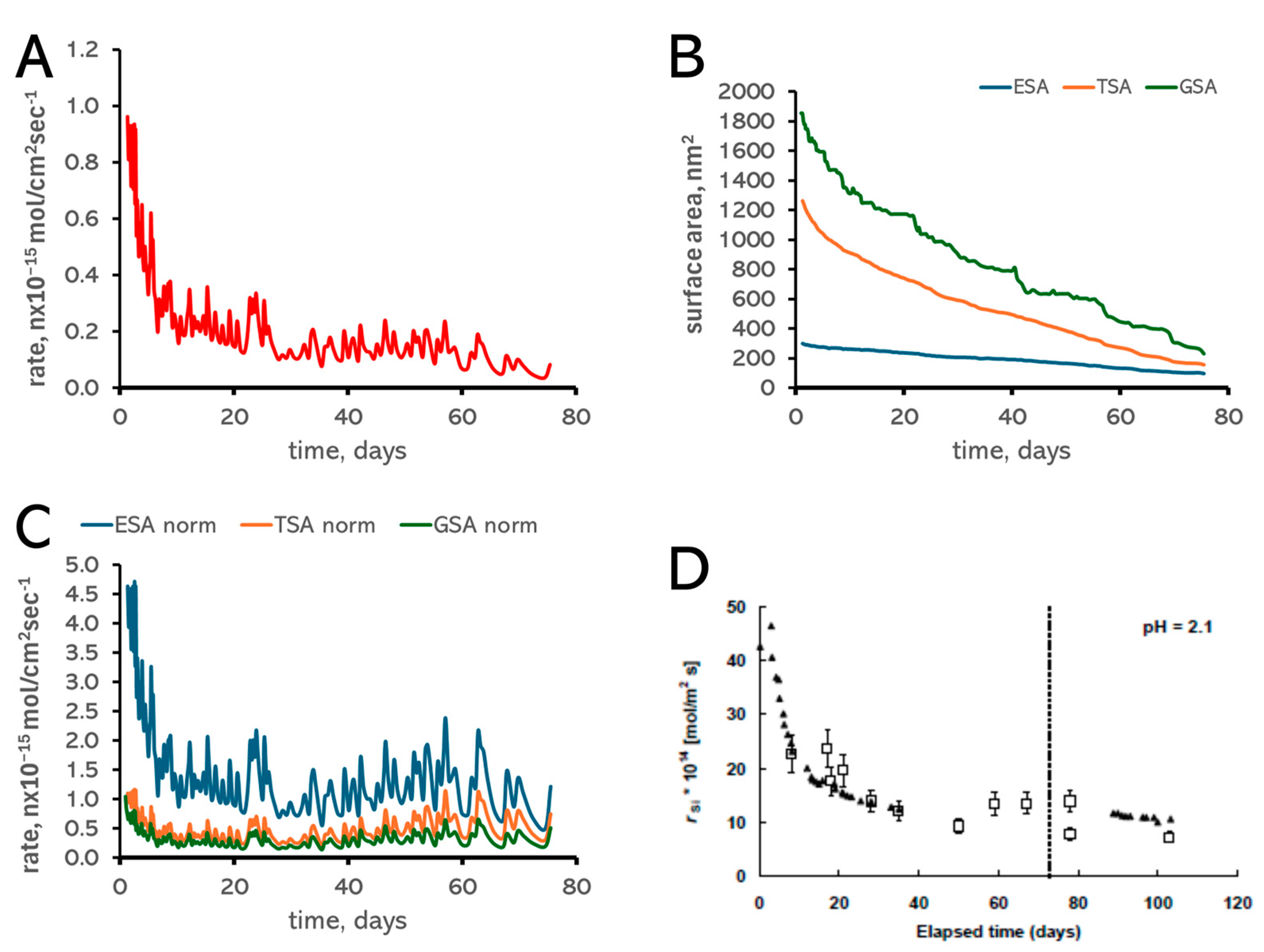
2.3. Dissolution Rate Calculations

The dissolution rate was calculated as material flux from the surface normalized by the surface area (SA). The material flux was calculated as a change $∆N$ in number of dissolved cations over the time step $∆t$. The units of the rates are moles/cm² s, in muscovite formula units Al₂(AlSi₃), six cations per unit formula. The formula for the rate calculation is as follows:

$$\mathrm{R}\left(\mathrm{S}\mathrm{A}\right)={\displaystyle \frac{∆N}{∆t}}{\displaystyle \frac{1}{N_a·SA·6}}$$

(2)

$N_a$ is Avogadro’s number. We used three types of surface areas for dissolution rate normalizations: (i) rates normalized by the edge surface area (ESA), (ii) rates normalized by the total surface area (aka “BET”) (TSA), and (iii) rates normalized by the geometric surface area (GSA).

Edge surface area is calculated as follows (Figure 2):

$$\mathrm{E}\mathrm{S}\mathrm{A}=\mathrm{P}\mathrm{e}\mathrm{r}\mathrm{i}\mathrm{m}\mathrm{e}\mathrm{t}\mathrm{e}\mathrm{r}(\mathrm{o}\mathrm{c}\mathrm{t}\mathrm{a}\mathrm{h}\mathrm{e}\mathrm{d}\mathrm{r}\mathrm{a}\mathrm{l} \mathrm{b}\mathrm{o}\mathrm{u}\mathrm{n}\mathrm{d}\mathrm{a}\mathrm{r}\mathrm{y})·\mathrm{T}\mathrm{O}\mathrm{T}\_\mathrm{h}\mathrm{e}\mathrm{i}\mathrm{g}\mathrm{h}\mathrm{t}$$

(3)

Total surface area is calculated as follows:

$$\mathrm{T}\mathrm{S}\mathrm{A}={\displaystyle \frac{{\mathrm{a}·\mathrm{b}·\mathrm{s}\mathrm{i}\mathrm{n}\left(\mathsf{\gamma }\right)·\mathrm{N}}_{\mathrm{T}}}{4}}+\mathrm{E}\mathrm{S}\mathrm{A}$$

(4)

where a, b, c, α, β, and γ are unit cell parameters, ${\mathrm{N}}_{\mathrm{T}}$ is the total number of tetrahedral atoms exposed at the surface. Every four tetrahedral surface atoms cover the elementary surface area $\mathrm{a}·\mathrm{b}·\mathrm{s}\mathrm{i}\mathrm{n}\left(\mathsf{\gamma }\right)$.

The lateral surface area (top and bottom) is summed up with the edge surface area to give TSA. Geometric surface area is calculated as a sum of the areas of parallelograms enclosing the entire nanoparticle according to the following formula:

$${GSA}_{NP}=2\left(A·B·sin\left(\gamma \right)+A·C·sin\left(\beta \right)+B·C·\mathrm{s}\mathrm{i}\mathrm{n}\left(\alpha \right)\right)$$

(5)

where A = X_max − X_min, B = Y_max − Y_min, Z = Z_max − Z_min are differences in absolute maximum and minimum atomic coordinates along Cartesian XYZ directions. The surface areas ESA, TSA, and GSA were calculated in nm² units.

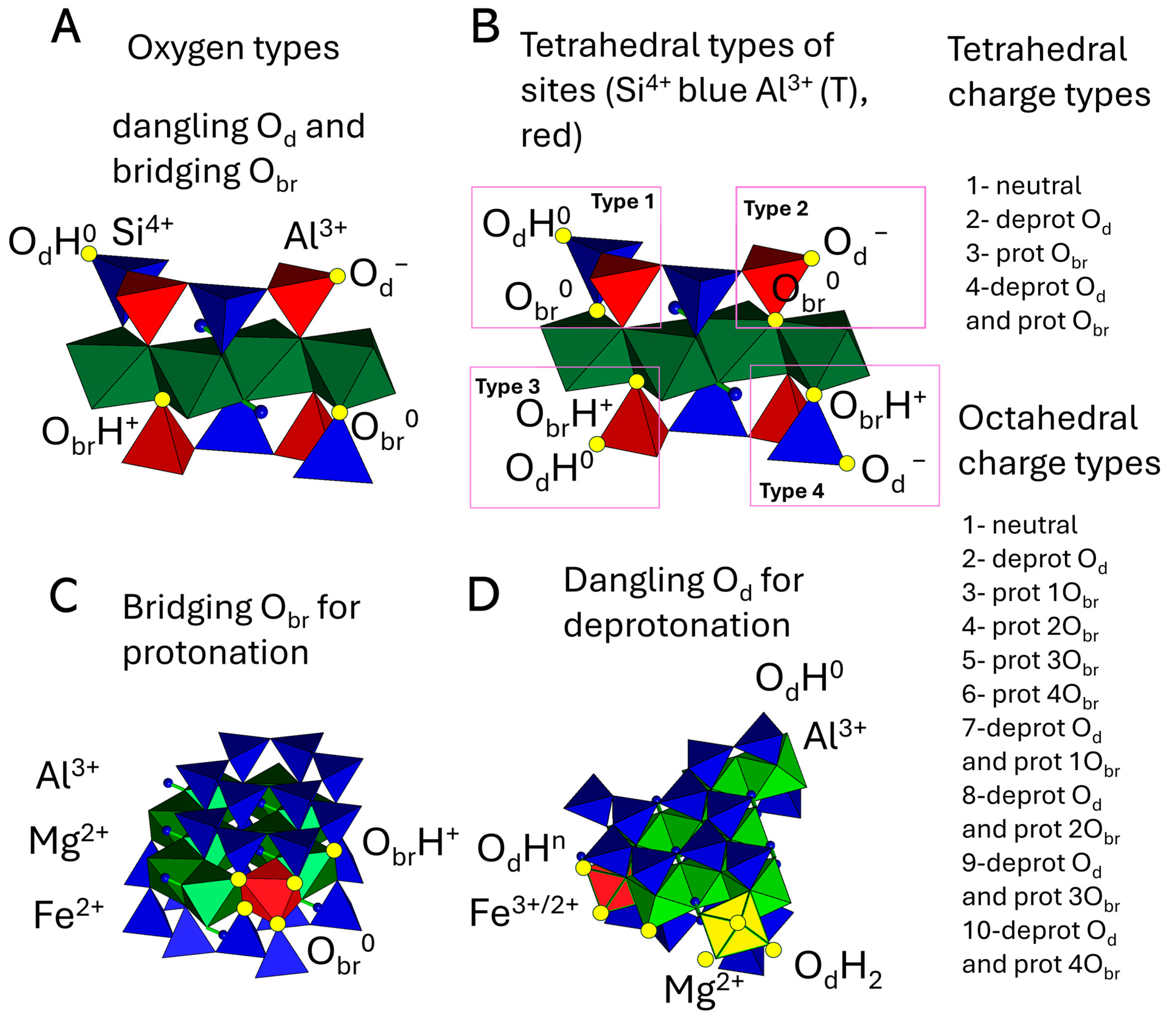
2.4. Acid–Base Property Modeling

The influence of pH on surface charge and dissolution rates of nanoparticles was modeled via the incorporation of deprotonation and protonation reactions for different surface sites (Figure 3). The reactions were assumed to be in equilibrium due to the fast activationless kinetics that are much faster (femtoseconds) [39] than the kinetics of silicate bond hydrolysis reaction with high activation barriers [40,41,42,43,44,45]. Both types of reactions are attributed to presence of surface oxygen atoms: dangling O_d formed as a result of bulk bond breaking within either tetrahedral or octahedral layers and bridging O_br atoms connecting tetrahedral and octahedral atoms (Figure 3A). I considered the following acid–base reactions characterized by their acidity constants $K_a$:

$$>M-{O_{d}H}^n\to >M-{O_d}^{n-1}+H^{+}$$

(6)

$$K_a={\displaystyle \frac{\left[>M-{O_d}^{n-1}\right]\left[H^{+}\right]}{\left[>M-{O_{d}H}^n\right]}}$$

(7)

$${\displaystyle \frac{\left[>M-{O_d}^{n-1}\right]}{\left[>M-{O_{d}H}^n\right]}}={10}^{pH-p{K}_a}$$

(8)

$$>M1-O_{br}{H}^{+}-M2\to M1-O_{br}-M2+H^{+}$$

(9)

$$K_a={\displaystyle \frac{\left[>M1-O_{br}-M2\right]\left[H^{+}\right]}{\left[>M1-O_{br}{H}^{+}-M2\right]}}$$

(10)

$${\displaystyle \frac{\left[>M1-O_{br}{H}^{+}-M2\right]}{\left[>M1-O_{br}-M2\right]}}={10}^{p{K}_a-pH}$$

(11)

The fraction of deprotonated sites according to the (Equation (8)) was implemented for tetrahedral (T) and octahedral (O) sites having at least one broken bond in a corresponding T or O layer, which can become deprotonated only one time per site. Every site appearing on the surface at the moment of losing the first relevant neighbor was selected as a candidate for the deprotonation reaction. Tetrahedral surface sites having a bridging O_br bond were selected as candidates for protonation reactions upon appearance of sites on the surface. All apical bridging bonds can become protonated. Connected octahedral atoms become also protonated as a result. A uniformly distributed random number was used to make a decision regarding protonation or deprotonation reaction. The values of pK_a used in the present study are shown in

Table 2. Acidity constants (pK_as) used in the KMC simulations. Please see explanations for the choice in the Results and Discussion, Section 3.4.

Site	pKa	Deprotonated/Protonated Site	Activation Energy Correction, kT Units
Si-OH0	7	Si-O−	−10
Al(T)-OH2	15	Al(T)-OH−	−7
Al(O)-(OH2)(OH)0	10	Al(O)-(OH)(OH)−	−10
Fe(III)-(OH2)(OH)0	9	Fe(III)-(OH)(OH)−	−10
Mg-(OH2)20	13	Mg-(OH2)(OH)−	−10
Si-O(br)-Al(O)	2	Si-O(br)H+-Al(O)	−15
Al(T)-O(br)-Al(O)	5	Al(T)-O(br)H+-Al(O)	−10
Si-O(br)-Mg(O)	2	Si-O(br)H+-Mg(O)	−10
Al(T)-O(br)-Mg(O)	5	Al(T)-O(br)H+-Mg(O)	−10
Si-O(br)-Fe(O)	2	Si-O(br)H+-Fe(O)	−10
Al(T)-O(br)-Fe(O)	5	Al(T)-O(br)H+-Fe(O)	−10

. There are four types of charged sites per each tetrahedral reactive class based on the numbers and types of neighbors, as introduced in [38] (Figure 3B). Octahedral atoms may have up to four O_br bonds of different types (Figure 3C), and dangling O_d (Figure 3D). As a result, there are ten possible charge states for each neutral reactive site class (Figure 3) based on topology of bonding. The corrections to the dissolution probabilities for charged sites were introduced by using activation energy corrections (Table 2):

$$P_i^{n_d{m}_H}=P_i^0·exp\left(-{\displaystyle \frac{n_d∆E_d}{kT}}\right)·exp\left(-{\displaystyle \frac{m_H∆E_H}{kT}}\right)$$

(12)

where $n_d=0,1$ is the number of deprotonated oxygen atoms at this stie for deprotonation reactions, 0 for neutral sites, 1 for deprotonated sites, $n_d=0,1$ for tetrahedral sites, the number of protonated oxygen atoms $m_H=0,1,2,3,4$ for octahedral sites.

3. Results and Discussion

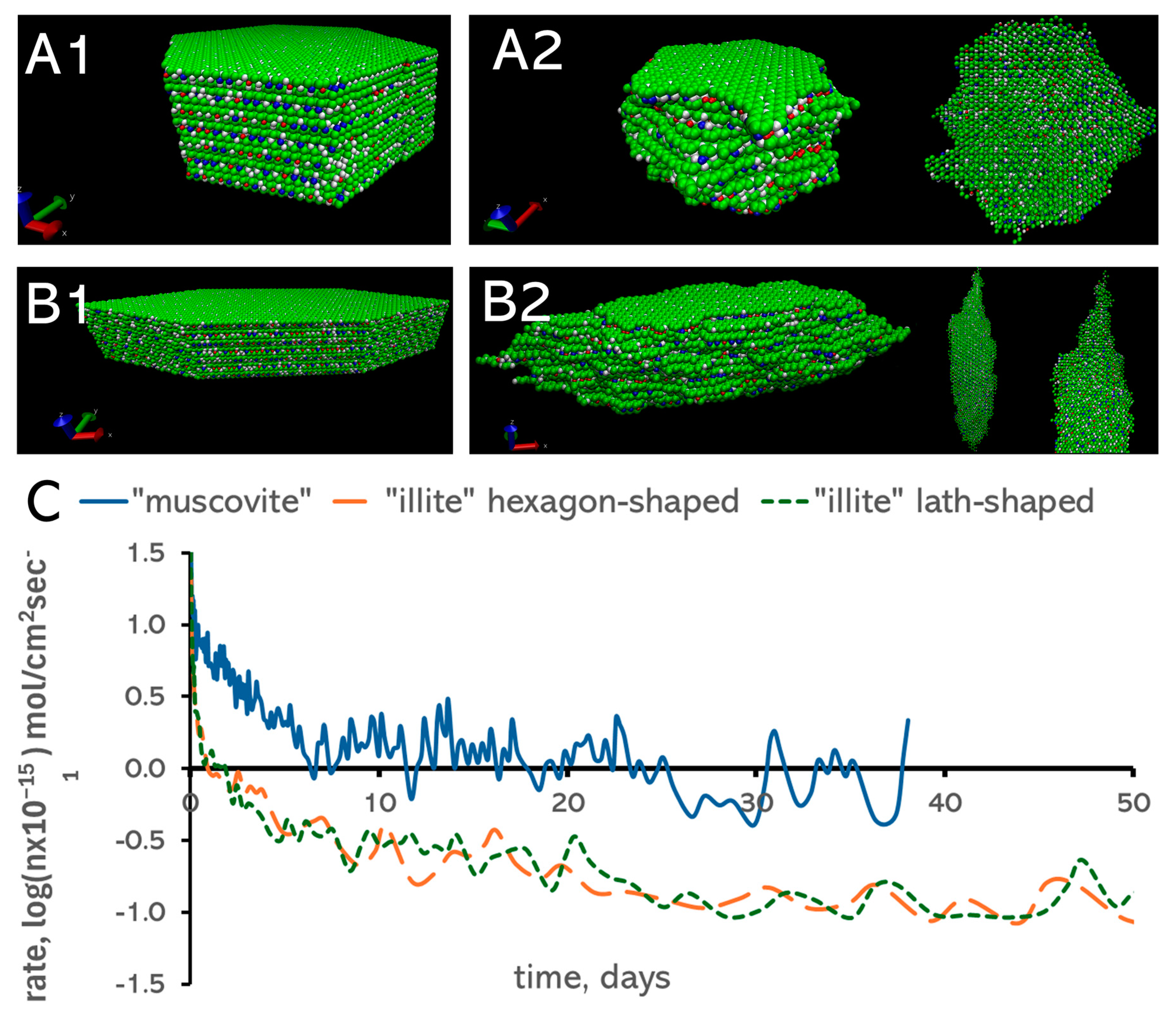
3.1. Surface Area Normalization

The normalization of material fluxes by a properly calculated surface area has a tremendous importance for calculation of dissolution rates. Depending on the choice of surface area type, rates derived from the same experiments may differ by significant orders of magnitude [51,52,53]. There are different types of surface areas presented in the literature: (i) total surface area (TSA), which is calculated based on the total number of surface sites and which is commonly measured using the BET (Brunauer–Emmett–Teller) method [54,55,56]. The BET method is based on measuring the amount of adsorbed gas, and the estimate may depend on the adsorption model involved [57]; (ii) geometric surface area (GSA), which is typically an approximation of mineral particle’s shape, spherical, rectangular, etc.; and (iii) edge surface area (GSA), specifically considered for phyllosilicates where the majority of the total area is occupied by basal faces with inert sites, and reactions of dissolution, adsorption, or crystal growth takes place at (hk0) faces. The question of which of the surface areas to use for normalization is largely dictated by the following factors: (i) whether the surface area of choice accurately represents locations where reactive fluxes are generated; (ii) if the chosen surface area is measured one time, whether it is expected not to substantially change during the measurement period.

All material fluxes produced in the current study showed a characteristic exponential decline over time (Figure 4A,C). Figure 4A represents rates calculated via normalization by initial (“BET”) total surface area (TSA), as it is a common practice in laboratory measurements of dissolution rates. The first question is whether this initially measured surface area is a good normalization parameter for clay minerals whose particle sizes range from nanometers to a few microns. Figure 4B shows gradual decline in all three types of KMC-derived surface areas over time for a 50 nm-sized nanoparticle (NP). Another question is which surface area type should be used for normalization, if we assume that we can either measure or predict how this surface area changes over time. As we can see from Figure 4B, total (TSA) and geometric (GSA) surface areas differ from the edge (ESA) surface area by two to three orders of magnitude. Kuwahara, 2008 [52], demonstrated the effect of surface area normalization by TSA and ESA, where ESA-normalized rates did not depend on the initial TSA value, in contrast to TSA-normalized rates. Figure 4C shows a comparison of KMC rates (this study) calculated based on the normalization of material fluxes by edge, total, and geometric surface areas (ESA, TSA, and GSA). The ESA-normalized rates show the highest values due to the low values of ESA in comparison to the other types of surface areas. There are no etch pit openings simulated in the present study, but even in this case, the value of the ESA would then change upon the opening of etch pits that expose additional amounts of (hk0) faces to the reactive solution contributing to ESA [38]. The normalization of material fluxes by the ESA for the phyllosilicate dissolution process thus provides an accurate estimate of rates, so we present all the rates normalized by ESA further on in this study.

Another important factor contributing to correct estimation of rates is temporal changes of the surface areas during the dissolution process. The pseudo “steady-state” observed in Figure 4C is thus supported by normalization by constantly changing surface areas (Figure 4B). In many cases, it is not possible to measure surface area change over time, and normalization is commonly applied using initial surface area, although in some cases final surface area was used because it is more relevant to the “steady-state” [58]. In the long run, this may unavoidably generate issues with rates never reaching a steady state, as discussed by Köhler et al. [51], Bibi et al. [59], and other authors. It has been demonstrated that illite dissolution rates have been decreasing in time and have never reached a steady state (Figure 4D). Temporal changes in surface area might not be the only factor influencing temporal changes in rates. Despite proper material flux normalization in this study, I obtained a very similar trend (Figure 4C) due to changes in nanoparticle morphology over time (see text below) and corresponding changes in reactive site densities.

3.2. Morphology of Nanoparticles

The morphology of nanoparticles may, in general, influence their reactive properties, as demonstrated in a previous KMC study for the adsorption of arsenate ions on hematite nanoparticles [60]. There are a wide range of clay mineral nanoparticles (NPs) morphologies documented in the literature [37,61,62]. They can be roughly classified into hexagonal (Figure 5A,F1), elongated (Figure 5B,E), and lath-shaped (Figure 5C,G) types, which were reproduced in the present KMC study. According to the results of the KMC simulations (this study), the dissolution process substantially alters the edges of NPs and makes them rough and irregular. Morphological alterations were observed for all three types of simulated NPs (Figure 5A–C). An interesting result for simulated systems is an apparent lack of a significant dependence of dissolution rates on the NP morphologies (Figure 5D). The temporal dynamics of rates for simulated NP dissolution shows irregular oscillations and surgical “spikes” for all three rate curves. These oscillations occur due to the retreat of terminating TOT layers and layer-by-layer retreat, giving surgical “spikes” in the material flux.

The dissolution of clay minerals in natural environments may rarely occur at the conditions of simulations, which are reproduced here for simplicity as mimicking “idealized” laboratory conditions suited for kinetic studies. Here, dissolving NPs are treated as a suspension of individual detached units in a flow-through reactor supporting far-from-equilibrium regime and constant pH values. At the condition of geological formations, illite is commonly found as fibrous bundles of elongated (Figure 5E) or lath-shaped (Figure 5G) NPs exposed to the pore fluid. Illite NPs commonly form complex textured networks of interviewed material filling intergranular pore space (Figure 5G). Therefore, the dissolution process and corresponding rates can be substantially different from those shown in Figure 5A–D. The major issue is the transport of dissolved material (silica, alumina, etc.) through the pore space and local saturation state. Another issue is that reactive surface sites exposed in such fibrous networks may have different kinetic behavior due to crystallographic constraints. NP aggregation and disaggregation may take place depending on local pH conditions and changes of edge surface charges. All these details should be taken into account for making any predictions for pore space alteration upon the dissolution and transport of clay mineral NPs in the pore space.

3.3. Chemical Composition Effects

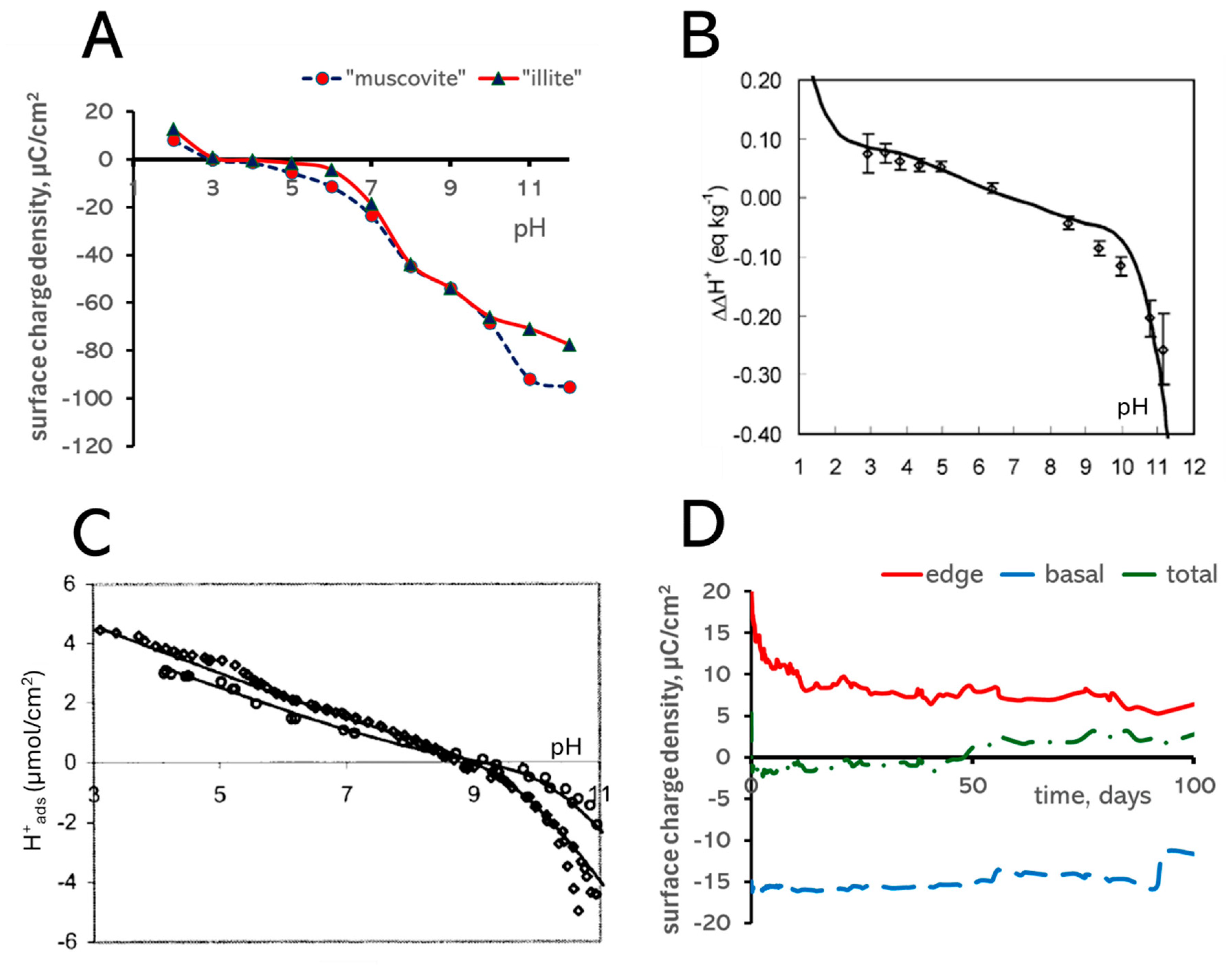
The incorporation of Mg²⁺ and Fe^2+/3+ into octahedral layers might have at least a two-fold effect on dissolution rates: (i) via generation of stronger bridging bonds and bonds within octahedral layers (Table 1); and (ii) via changing populations of protonated and deprotonated sites due to different acidity constants (see Table 2). Both effects are implemented into our KMC model as parameter values for bond-breaking and pK_a values listed in Table 1 and Table 2.

Figure 6 demonstrates the results of KMC runs on NPs of “illite” type. There is no principal difference in NPs morphologies between this type and the “muscovite” type (see Figure 5). However, the edges of NPs tend to be slightly rougher and more irregular for “illite” compositions (Figure 6A2,B2) due to the formation of more stable Mg-Fe-Al clusters within octahedral layers. The formation of sharp “fibrous” ends is also characteristic for “illite” compositions, as is shown in Figure 6B2, compared to the SEM observations of “fibrous” illite NPs shown in Figure 5E.

The dissolution rates between “muscovite” and “illite” compositions differ by about one to two orders of magnitude. It is important to note that the magnitude of this difference strongly depends on the choice of bond breaking parameters presented in Table 2. Another noticeable effect of “illite” composition is the smooth character of rate oscillations without higher-frequency spikes characteristic for the “muscovite” type (Figure 6C). This effect is interesting and counterintuitive, because the presence of Mg and Fe introduces new types of sites with different reactivity. This effect is apparently generated by the dominance of Mg and Fe sites at the octahedral edges controlling the reaction rate, while the “muscovite”-type dissolution rate is controlled by the directionality of periodic bond chains (PBCs). The PBCs in both types are rotated by 120° to each other due to the lattice structure of 2M₁ crystallographic polytype. As a result, PBCs in the adjacent TOT layers limit each other’s retreat (see more detailed explanation in [63]). The locations where dissolution takes place and triggers dissolution of the adjacent kinetically dependent TOT layers is thus stochastically chosen. This effect is apparently hindered for the “illite” type where the detachment of uniformly randomly distributed Mg and Fe sites controls the release of atoms. The choice of a specific initial NP’s morphology, e.g., hexagonal or lath-shaped, does not substantially influence the values of dissolution rates.

3.4. Surface Charge

Surface charge plays an incredibly important role for mineral–water interface reactions. The adsorption of ions, crystal dissolution and growth depend on charge of surface sites where reactions take place. The overall surface charge influences the structure of water layers adsorbed at the mineral–water interface, as well as water dissociation, and determines the structure of the surface electric double layer (EDL) with aqueous ions adsorbed as outer-sphere complexes. Protonation and deprotonation reactions on clay mineral NPs modify their surface charge depending on pH conditions [64,65,66,67,68]. Since these reactions are directly included in our KMC model, the information on overall surface charge as a function of pH (so-called “titration curves”) can be accessed and compared to titration curves measured for clay minerals at laboratory conditions.

Figure 7 demonstrates modeled and experimentally obtained titration curves and surface charge changes over time. The behavior of these curves bears important information about populations of statistically dominating charged sites and their acid–base properties. The charge is essentially a function of pH value according to Equations (6)–(11). These equations define fractions of protonated and deprotonated sites as functions on pH and the acidity constants, pK_as. Acidity constants are individual for different types of sites, as listed in Table 2. At pH = pK_a, the number of de/protonated sites is half of the total sites of that type. The number of charged sites increases with increasing pH for deprotonation reaction and decreases for protonation reaction. The point pH = pK_a is the inflection point of the titration curve. If the crystalline surface contains sites with different pK_as present in statistically significant amounts, several inflection points may appear on titration curves, as can be seen in Figure 7A,B.

The construction of a proper and accurate acid–base model for clay minerals can be a tedious task. There is a large variety of clay minerals that may contain different stoichiometric numbers of reactive sites with different pK_as. The number of site types even for one specific clay mineral type can be quite large (see, for example, [66,67,69]). Table 3 presents a compilation of different surface sites considered by authors who have studied acid–base properties of clay minerals. The tapestry of sites is much vaster than those considered in the present KMC model. Interestingly enough, in most cases, protonation for bridging O_br sites, as shown in Figure 3, is not considered, with a few exceptions, e.g., as in the recent publications by Gao et al. [71]. Thus, the construction of an acid–base model for a mineral surface charge consists of the following steps: (1) the definition of the surface sites participating in protonation–deprotonation reactions in a sensible pH range, e.g., 0–13; (2) the determination of the number of de/protonation steps at those sites, commonly described similar to Equations (6)–(11), where we assumed only one de/protonation step per site type; and (3) the estimation of acidity constants (pK_as). The correct estimation of pK_as is, therefore, crucial for a proper acid–base model.

There are a variety of methods used to calculate pK_a values: the CD-MUSIC [72] approach based on the bond-valence theory by Hiemstra et al. [73,74,75,76,77], the ab initio/DFT approach introduced by Sulpizi and Sprik [78], the experimental determination of “empirical” or “apparent” acidity constants derived from titration curves [79], and a combination of bond valence approach and experimental titration [66,69,77]. Although laboratory titration curves show only an integrated result of all site acid–base behavior, their inflection points may provide valuable information about pK_a values. Figure 7C shows a titration curve for gibbsite, Al(OH)₃ mineral, whose structure is formed by octahedral layers. There is a clearly visible inflection point at pH = 9–12. Our acid–base model has pK_a = 10 for deprotonation at Al sites in the gibbsite layer, which provides the same inflection at pH = 10 (Figure 7A). Another important inflection point occurs at pH = 7, caused by the deprotonation of dangling O_d bonds at Si sites. Although data from Table 3 show a variety of pK_a values for the same types of sites depending on the calculation method, empirical inflection points from experimental titration curves [80] as well as Grand Canonical Monte Carlo simulations for illite [81] show an inflection point around pH = 7. Table 4 presents a few experimental data points with visibly detectable inflection points from different studies. In many cases, only two or three inflection points can be clearly identified, probably caused by the deprotonation of dangling O_d bonds at Si and octahedral Al sites that are abundant on clay mineral surfaces. The third important inflection point detectable on experimental titration curves (Figure 7B) is around pH = 1–2. This inflection point is typically sharp and not always detectable in common titration curves with pH ranges 3–12. The steep slope of the titration curve around pH = 1–2 indicates a statistically significant amount of surface sites participating in protonation reaction. Although there can be various candidates considered for this effect, we would like to point out that bridging M-O_br-M sites also might become protonated and are also massively abundant at charged (hk0) faces.

The majority of bond-valence models for clay minerals do not incorporate protonation of bridging Si/(Al(T)-O_br-M(O) bonds. Thus, all bonds listed in Table 3 are for either dangling Si/Al(T) bonds or for bridging bonds in the octahedral layer. However, recent DFT studies provide a pK_a for the apical Si-O_br-Al(O) bond as 1.7 [71], which is within experimentally observed inflection point location pH = 2. Since we used pK_a = 2 for our acid–base model for all Si-O_br-M(O) sites (Table 2), we observe the same inflection point at around pH = 2 (Figure 7A). The value pK_a = 5 for all Al(T)-O_br-M(O) sites (Table 2) generates an additional shallow inflection point around pH = 5 for NPs of “muscovite” type and barely noticeable inflection point for NPs of “illite” type at the same pH. This difference is generated by larger population of Al(T) sites for “muscovite”-type NPs. We suggest that the protonation of apical bridging Si/(Al(T)-O_br-M(O) bonds is a ubiquitous process for most of clay minerals, according to the sharp inflection around pH = 1–2 appearing on the majority of titration curves. There is also a possibility that dangling bonds or bridging bonds in the octahedral layer attach additional protons. We did not consider this possibility in the present study, where only one de/deprotonation step per site in the pH range 2–12 was considered.

While pK_a values for dangling Si-O_dH and Al(O)-O_dH bonds are roughly around 6–8, and values of 8–10 are largely assumed by the research community, pK_a values for the other sites are not very consistent between the authors and methods used; see Table 3 for details. For this reason, the pK_a values for the Mg and Fe sites used in the present model are not much different from the Si and Al(O) sites (Table 2). pK_a for Mg-O_dH₂ deprotonation was set to 13, thus giving an inflection point on the “illite” NP titration curve, which is not observed for “muscovite” NP (Figure 7A). The same inflection point is observed on an experimental titration curve for montmorillonite (Figure 7B), a Mg-bearing clay mineral. A DFT study by Gao et al. [71] also provides a pKa = 13.2 value for this site. We, therefore, suggest that pK_a =13 for Mg-O_dH₂ deprotonation is a justified and reasonable value.

Table 3. Acidity constants (pK_as) for different sites at phyllosilicate surfaces (literature review).

Site	pKa	Mineral	Face	Formula(O)(T)	Method/Source
Si-OH	7.0 ± 0.7	montmorillonite	(010)	(Al3.5Mg0.5) (Si)	DFT-MD [82]
Al-(OH2)(OH)	8.3 ± 1.0	montmorillonite	(010)	(Al3.5Mg0.5) (Si)	DFT-MD [82]
Al-(OH2)2	3.1 ± 0.5	montmorillonite	(010)	(Al3.5Mg0.5) (Si)	DFT-MD [82]
Mg-(OH2)2	13.2 ± 0.5	montmorillonite	(010)	(Al3.5Mg0.5) (Si)	DFT-MD [82]
Fe(III)-(OH2)2	1.2 ± 0.7	Nontronite	(010)	(Fe3Al1) (Si8)	DFT-MD [83]
Fe(III)-(OH2)(OH)	4.4 ± 0.3	Nontronite	(010)	(Fe3Al1) (Si8)	DFT-MD [83]
Si-OH	8.7 ± 1.4	Nontronite	(010)	(Fe3Al1) (Si8)	DFT-MD [83]
Fe(III)-(OH2)2	1.2 ± 0.5	Fe-montmorillonite	(010)	(Fe0.5Al3) (Si8)	DFT-MD [83]
Fe(III)-(OH2)(OH)	5.1 ± 1.0	Fe-montmorillonite	(010)	(Fe0.5Al3) (Si8)	DFT-MD [83]
Si-OH	8.6 ± 1.0	Fe-montmorillonite	(010)	(Fe0.5Al3) (Si8)	DFT-MD [83]
≡Si–OHn	9.1	montmorillonite	-	(Al,Fe,Mg) (Si,Al)	CD-MUSIC [66]
≡Al–OHn	10.5	montmorillonite	-	(Al,Fe,Mg) (Si,Al)	CD-MUSIC [66]
≡Mg–OHn	12.7	montmorillonite	-	(Al,Fe,Mg) (Si,Al)	CD-MUSIC [66]
≡Fe(III)–OHn	8.9	montmorillonite	-	(Al,Fe,Mg) (Si,Al)	CD-MUSIC [66]
≡SiAl–Ohn	7.7	montmorillonite	-	(Al,Fe,Mg) (Si,Al)	CD-MUSIC [66]
≡SiMg–OHn	9.8	montmorillonite	-	(Al,Fe,Mg) (Si,Al)	CD-MUSIC [66]
≡SiFe(III)–OHn	6.1	montmorillonite	-	(Al,Fe,Mg) (Si,Al)	CD-MUSIC [66]
≡AlAl–OHn	5.1	montmorillonite	-	(Al,Fe,Mg) (Si,Al)	CD-MUSIC [66]
≡AlMg–OHn	7.3	montmorillonite	-	(Al,Fe,Mg) (Si,Al)	CD-MUSIC [66]
≡AlFe(III)–OHn	3.5	montmorillonite	-	(Al,Fe,Mg) (Si,Al)	CD-MUSIC [66]
Al-(OH2)2	9.5 ± 0.8	Gibbsite	(100)	Al	DFT-MD [84]
Si-OH	6.8 ± 0.4	pyrophyllite	(010)	(Al)(Si)	DFT-MD [85]
Al-(OH2)	7.6 ±1.3	pyrophyllite	(010)	(Al)(Si)	DFT-MD [85]
Al(T)-OH	15.1	-	Si,Al	(Al) (Si,Al)	DFT-MD [86]

Table 3. Acidity constants (pK_as) for different sites at phyllosilicate surfaces (literature review).

Site	pKa	Mineral	Face	Formula(O)(T)	Method/Source
Si-OH	7.0 ± 0.7	montmorillonite	(010)	(Al3.5Mg0.5) (Si)	DFT-MD [82]
Al-(OH2)(OH)	8.3 ± 1.0	montmorillonite	(010)	(Al3.5Mg0.5) (Si)	DFT-MD [82]
Al-(OH2)2	3.1 ± 0.5	montmorillonite	(010)	(Al3.5Mg0.5) (Si)	DFT-MD [82]
Mg-(OH2)2	13.2 ± 0.5	montmorillonite	(010)	(Al3.5Mg0.5) (Si)	DFT-MD [82]
Fe(III)-(OH2)2	1.2 ± 0.7	Nontronite	(010)	(Fe3Al1) (Si8)	DFT-MD [83]
Fe(III)-(OH2)(OH)	4.4 ± 0.3	Nontronite	(010)	(Fe3Al1) (Si8)	DFT-MD [83]
Si-OH	8.7 ± 1.4	Nontronite	(010)	(Fe3Al1) (Si8)	DFT-MD [83]
Fe(III)-(OH2)2	1.2 ± 0.5	Fe-montmorillonite	(010)	(Fe0.5Al3) (Si8)	DFT-MD [83]
Fe(III)-(OH2)(OH)	5.1 ± 1.0	Fe-montmorillonite	(010)	(Fe0.5Al3) (Si8)	DFT-MD [83]
Si-OH	8.6 ± 1.0	Fe-montmorillonite	(010)	(Fe0.5Al3) (Si8)	DFT-MD [83]
≡Si–OHn	9.1	montmorillonite	-	(Al,Fe,Mg) (Si,Al)	CD-MUSIC [66]
≡Al–OHn	10.5	montmorillonite	-	(Al,Fe,Mg) (Si,Al)	CD-MUSIC [66]
≡Mg–OHn	12.7	montmorillonite	-	(Al,Fe,Mg) (Si,Al)	CD-MUSIC [66]
≡Fe(III)–OHn	8.9	montmorillonite	-	(Al,Fe,Mg) (Si,Al)	CD-MUSIC [66]
≡SiAl–Ohn	7.7	montmorillonite	-	(Al,Fe,Mg) (Si,Al)	CD-MUSIC [66]
≡SiMg–OHn	9.8	montmorillonite	-	(Al,Fe,Mg) (Si,Al)	CD-MUSIC [66]
≡SiFe(III)–OHn	6.1	montmorillonite	-	(Al,Fe,Mg) (Si,Al)	CD-MUSIC [66]
≡AlAl–OHn	5.1	montmorillonite	-	(Al,Fe,Mg) (Si,Al)	CD-MUSIC [66]
≡AlMg–OHn	7.3	montmorillonite	-	(Al,Fe,Mg) (Si,Al)	CD-MUSIC [66]
≡AlFe(III)–OHn	3.5	montmorillonite	-	(Al,Fe,Mg) (Si,Al)	CD-MUSIC [66]
Al-(OH2)2	9.5 ± 0.8	Gibbsite	(100)	Al	DFT-MD [84]
Si-OH	6.8 ± 0.4	pyrophyllite	(010)	(Al)(Si)	DFT-MD [85]
Al-(OH2)	7.6 ±1.3	pyrophyllite	(010)	(Al)(Si)	DFT-MD [85]
Al(T)-OH	15.1	-	Si,Al	(Al) (Si,Al)	DFT-MD [86]

The shapes of titration curves for clay minerals are generated primarily by the pH-sensitive charge of edge faces of nanoparticles. Since basal faces do not have broken bonds, protonation is very unlikely and not incorporated into the model. The charge of basal faces stems from Si⁴⁺/Al³⁺ substitution in the tetrahedral layers, and overall NP charge density does not much depend on time (Figure 7D). Since edges of nanoparticles are positively charged at low pH while basal faces are negatively charged, nanoparticles may aggregate at these pH conditions. Edge and basal faces at high pH conditions are both negatively charged, thus generating repulsive forces [34]. The charge densities in KMC simulations normalized by ESA were quite stable over time (Figure 7D), depending only on the populations of edge sites exposed, which changed in the beginning of the simulations when NPs’ habits evolved from cut crystals to pseudo “steady-state” morphologies.

As we can see from the discussion above, the surface charge, titration curves, and populations of de/protonated sites can all be determined from a properly chosen acid–base model and acidity constant values. Overall, there is a huge microcosm of sites at clay mineral surfaces with a wide range of acidity constants (see Table 3), as has been studied for a long time by Bourg, Tournassat, Liu, Guo, and other authors [66,67,68,69,71,82,83,86,87,88]. The implementation of such diversity into a KMC model is possible but is out of the scope of the present test-case model. It can be undertaken, however, in the future to utilize the full capacity of the method. The sole use of pK_a constants and simplistic site balance equations such as Equations (6)–(11) is definitely not sufficient due to electrostatic interactions between the charged sites and influence of background electrolytes, as has been addressed by Grand Canonical Monte Carlo (GCMC) models [64,65,89,90]. The GCMC approach can be successfully combined with the KMC approach to study the pH-control of dissolution rates, as it has been demonstrated by Kurganskaya and Churakov [46]. Future refinements of acid–base models suitable for KMC simulations are thus ultimately required.

Table 4. Inflection points at pH-dependent zeta-potential curves for different phyllosilicate minerals, experimental studies and Grand Canonical Monte Carlo (GCMC) simulations.

Mineral	Inflection Points	Background Electrolyte	Tetrahedral	Octahedral	Method
montmorillonite	5/8	0.01 M NaCl	Si	Al,Mg	Exp [91]
montmorillonite	5/8	0.02 M NaCl	Si3.98Al0.02	Al1.55Fe(III)0.09Fe(II)0.08Mg0.28	Exp [69]
illite	6.3/10.6	0.001 M NaCl	Si6.89Al1.11	Al2.82Fe0.57Mg0.44	Exp [80]
illite	7/10.7	0.001 M NaCl	Si7.70Al0.3	Al0.28Fe2.71Mg0.86	Exp [80]
hematite	7	0.1 M NaClO4	-	Fe	Exp [92]
pyrophillite	3.8/9	0.1 mM 1-1 salt	Si	Al	GCMC [81]
montmorillonite	5/9	0.1 mM 1-1 salt	Si	Al3.5Mg0.5	GCMC [81]
Illite	6.5/9.5	0.1 mM 1-1 salt	Si,Al	Al,Fe,Mg	GCMC [81]

Table 4. Inflection points at pH-dependent zeta-potential curves for different phyllosilicate minerals, experimental studies and Grand Canonical Monte Carlo (GCMC) simulations.

Mineral	Inflection Points	Background Electrolyte	Tetrahedral	Octahedral	Method
montmorillonite	5/8	0.01 M NaCl	Si	Al,Mg	Exp [91]
montmorillonite	5/8	0.02 M NaCl	Si3.98Al0.02	Al1.55Fe(III)0.09Fe(II)0.08Mg0.28	Exp [69]
illite	6.3/10.6	0.001 M NaCl	Si6.89Al1.11	Al2.82Fe0.57Mg0.44	Exp [80]
illite	7/10.7	0.001 M NaCl	Si7.70Al0.3	Al0.28Fe2.71Mg0.86	Exp [80]
hematite	7	0.1 M NaClO4	-	Fe	Exp [92]
pyrophillite	3.8/9	0.1 mM 1-1 salt	Si	Al	GCMC [81]
montmorillonite	5/9	0.1 mM 1-1 salt	Si	Al3.5Mg0.5	GCMC [81]
Illite	6.5/9.5	0.1 mM 1-1 salt	Si,Al	Al,Fe,Mg	GCMC [81]

3.5. pH Control of Dissolution Rates

Systematic runs of KMC simulations at different pH values in this study were put together to obtain pH-dependence curves for dissolution rates (Figure 8A). The asymmetric V-shape is observed for both “muscovite” and “illite” NPs, with a difference of about 1.5–2.5 orders of magnitude, and a steeper curve around pH = 5 for “muscovite” NPs due to the higher density of Al(T), which has pK_a = 5 in the present model (Table 2). This pK_a value was chosen in this study for purely illustrative purposes, to show the influence of this parameter on the pH-dependence rate curve.

The same V-shape is observed for a wide range of clay minerals, e.g., various dioctahedral smectites, which dissolution rates were experimentally measured (Figure 8B) in different laboratories. The linear interpolation curve (red line) in Figure 8B was calculated by the authors for montmorillonite, a Mg-bearing clay mineral without or with a low amount of Al(T), which roughly corresponds to the composition of the “illite” NP. The pH-dependence of rate for the “illite” NP (Figure 8A) appears to behave similarly to the interpolation curve calculated for montmorillonite (Figure 8B).

The V-shape of the pH-dependence curves stems from a simple fact established by DFT simulations early on: activation barriers of bond hydrolysis for silicate minerals are substantially lower for both protonated and deprotonated sites [41,42,94,95,96]. The empirical rate law relating dissolution rates and proton activity appeared in the following form in the 1980s [97,98]:

$$Rate=k{a}_{H^{+}}^n$$

(13)

where $a_{H^{+}}^n$ is proton activity taken in some empirical power $n$, and $k$ is the proportionality constant. This concept was commonly extended to a longer form incorporating activities of aqueous hydroxyl species and water, some exponential pre-factors, and activation energy parameters [48]:

$$r=A_{H}exp\left(-{\displaystyle \frac{E_{{AH}^{+}}}{RT}}\right)a_{H^{+}}^{0.6}+A_{H_{2}O}exp\left(-{\displaystyle \frac{E_{A{H}_{2}O}}{RT}}\right)+A_{OH}exp\left(-{\displaystyle \frac{E_{{AOH}^{-}}}{RT}}\right)a_{{OH}^{-}}^{0.6}$$

(14)

Three different terms of the sum above represent parallel rate contributions from “proton-attack”(denoted by H⁺), “water-attack” (denoted by H₂O), and “hydroxyl attack” (denoted by OH⁻) on surface sites considered as identically reactive entities. Surface sites in this type of models are not differentiated by their reactive properties based on bond topologies, as it is studied and discussed in the previous model for phyllosilicate dissolution [38] or by acid–base properties (e.g., pK_a values) which have different populations depending on pH. These kinds of rate laws can be considered rather empirical and macroscopic since they are not backed up by a relevant diverse microcosm of sites discussed above. These rate laws, however, may have relevance under an assumption of one statistically dominant type of site, which may protonate and deprotonate, and whose density reaches a steady state, which is rarely the case for the majority of minerals [99,100,101]. As it is mentioned above, the dissolution of clay minerals rarely reaches a steady state, although at some point, properly normalized material fluxes may provide pseudo “steady-state” values, as we observed in KMC simulations in this study. The terms attributed to “proton attack” or “hydroxyl attack” may indeed be mechanistically related to the proton-involved reactions and site charge, and corresponding changes in activation energies of bond hydrolysis. However, pH-sensitive titration curves with many inflection points clearly indicate more than one site involved in charging and dissolution processes. As has been shown in the previous KMC studies of phyllosilicate dissolution [38], there are three different edge and kink sites active at three different crystallographic directions. Therefore, kinetic models described by Equation (13) or (14) are not sufficient even under assumptions for single rate-controlling sites where density is a constant value. If densities of reactive sites become time-dependent parameters, corrections are required, as was completed by Kurganskaya and Luttge for calcium carbonate [102]. An analogous rate equation can be introduced here as follows:

$$Rate={\sum }_{i=1}^n\left[k_i^{dp}{·N}_{dp}\left(t,pH,{{p{K}_a}^i,∆\mu }_i,C_{j=1..m}\right)+k_i^p{·N}_p\left(t,pH,{{p{K}_a}^i,∆\mu }_i,C_{j=1..m}\right){+k}_i^w{·N}_w\left(pH,{p{K}_a}^i,{∆\mu }_i,C_{j=1..m}\right)\right]·\left(1-e^{{\displaystyle \frac{{∆\mu }_i}{kT}}}\right)$$

(15)

where n is the number of kinetically contributing types of reactive sites, typically kink sites of various types, abbreviations $dp$, $p$, $w$ are attributed to “deprotonated”, “protonated”, and “neutral” states of sites, which should be extended to more mixed states as considered in this model, $k_i^{p,dp,w}$ denote molecular reaction rate constants that can be derived from ab initio studies, e.g., as in Schliemann and Churakov [40,103], $t$ is time, ${∆\mu }_i$ are chemical potential differences between dissolved species and corresponding surface sites, and $C_{j=1...m}$ are concentrations of other ions, e.g., background electrolytes, that may influence reactive site densities. All the parameters in this equation can be obtained from ab initio simulations and thermodynamic calculations, or direct measurements. The only parameter type that is difficult to measure and predict is condition-dependent numbers of sites. Properly set simulations, e.g., kinetic Monte Carlo, may substantially help in determining these parameters’ values.

4. Summary and Conclusions

The kinetic Monte Carlo (kMC) model previously developed for phyllosilicate dissolution is extended further to include clay mineral nanoparticles of arbitrary composition and the pH-dependence of dissolution rates. The new model incorporates acid–base properties of surface sites based on their acidity constants, pK_as, for dangling M-O_dH bonds in tetrahedral and octahedral layers, as well as bridging apical Si/Al(T)-O_br-M(O) bonds. The populations of charged sites at pH = 2–12 are calculated based on simple equilibrium equations. The constructed titration curves show major inflexion points observed in titration curves derived from experiments. Decrease in bond hydrolysis activation energy for deprotonated and protonated sites is a well-known fact from numerous ab initio/DFT calculations available in the literature. This effect is incorporated into the kMC model, where populations of de/protonated sites are adjusted according to the pH value. The systematic runs of kMC simulations at different pH values provided an asymmetric V-shaped pH-dependence curve of dissolution rates known for a long time from experimental data. This result clearly indicates the existence of massive protonation reactions around pH = 0–3, as it supported by assumed protonation of bridging apical Si/-O_br-M(O) bonds in the present kMC model. The new refined rate law is offered to cover relevant parameters and controls of dissolution process. Despite the complexity of clay mineral–water interface structure, consistent, reliable, and robust models of acid–base behavior and properly parameterized kinetic Monte Carlo (kMC) models might significantly help us to understand and predict the behavior of these materials in different chemical and geochemical environments. The ability to develop such models allows us not only to access reactive and sorbent properties of clay minerals, but also to develop novel layered nanomaterials with targeted functionality, for example, for adsorption of toxic ions and radionuclides at desired environmental conditions. This endeavor might require collective efforts in ab initio, molecular dynamics, Grand Canonical and kinetic Monte Carlo simulations, as well as other types of simulations, acid–base surface speciation modeling, and dedicated experimental verification of models. The kMC approach in a combination to experimental methods can be used as a hypothesis-testing tool for the role of selected surface sites in reactive properties of clay mineral–water interfaces.

References

1. Wang, C.; Myshkin, V.F.; Khan, V.A.; Panamareva, A.N. A Review of the Migration of Radioactive Elements in Clay Minerals in the Context of Nuclear Waste Storage. J. Radioanal. Nucl. Chem. 2022, 331, 3401–3426. [Google Scholar] [CrossRef]
2. Churakov, S.V.; Gimmi, T.; Unruh, T.; Van Loon, L.R.; Juranyi, F. Resolving Diffusion in Clay Minerals at Different Time Scales: Combination of Experimental and Modeling Approaches. Appl. Clay Sci. 2014, 96, 36–44. [Google Scholar] [CrossRef]
3. Kalinichev, A.G.; Loganathan, N.; Wakou, B.F.N.; Chen, Z. Interaction of Ions with Hydrated Clay Surfaces: Computational Molecular Modeling for Nuclear Waste Disposal Applications. Procedia Earth Planet. Sci. 2017, 17, 566–569. [Google Scholar] [CrossRef]
4. Murray, H.H. Overview—Clay Mineral Applications. Appl. Clay Sci. 1991, 5, 379–395. [Google Scholar] [CrossRef]
5. Rehman, A.; Rukh, S.; Ayoubi, S.A.; Khattak, S.A.; Mehmood, A.; Ali, L.; Khan, A.; Malik, K.M.; Qayyum, A.; Salam, H. Natural Clay Minerals as Potential Arsenic Sorbents from Contaminated Groundwater: Equilibrium and Kinetic Studies. Int. J. Environ. Res. Public Health 2022, 19, 16292. [Google Scholar] [CrossRef] [PubMed]
6. Uddin, M.K. A Review on the Adsorption of Heavy Metals by Clay Minerals, with Special Focus on the Past Decade. Chem. Eng. J. 2017, 308, 438–462. [Google Scholar] [CrossRef]
7. Carretero, M.I. Clay Minerals and Their Beneficial Effects upon Human Health. A Review. Appl. Clay Sci. 2002, 21, 155–163. [Google Scholar] [CrossRef]
8. Biswas, B.; Grathoff, G.; Naidu, R.; Warr, L.N. The Multidisciplinary Science of Applied Clay Research: A 2021–2023 Bibliographic Analysis. Appl. Clay Sci. 2024, 258, 107471. [Google Scholar] [CrossRef]
9. Cygan, R.T.; Liang, J.-J.; Kalinichev, A.G. Molecular Models of Hydroxide, Oxyhydroxide, and Clay Phases and the Development of a General Force Field. J. Phys. Chem. B 2004, 108, 1255–1266. [Google Scholar] [CrossRef]
10. Cygan, R.T.; Greathouse, J.A.; Kalinichev, A.G. Advances in Clayff Molecular Simulation of Layered and Nanoporous Materials and Their Aqueous Interfaces. J. Phys. Chem. C 2021, 125, 17573–17589. [Google Scholar] [CrossRef]
11. Baston, G.M.N.; Berry, J.A.; Brownsword, M.; Cowper, M.M.; Heath, T.G.; Tweed, C.J. The Sorption of Uranium and Technetium on Bentonite, Tuff and Granodiorite. In Proceedings of the Symposium—Scientific Basis for Nuclear Waste Management XVIII, Kyoto, Japan, 23–27 October 1994; Volume 353. [Google Scholar]
12. Churakov, S.V.; Hummel, W.; Fernandes, M.M. Fundamental Research on Radiochemistry of Geological Nuclear Waste Disposal. Chimia 2020, 74, 1000. [Google Scholar] [CrossRef] [PubMed]
13. Zaoui, A.; Sekkal, W. Can Clays Ensure Nuclear Waste Repositories? Sci. Rep. 2015, 5, 8815. [Google Scholar] [CrossRef] [PubMed]
14. Lee, S.Y.; Tank, R.W. Role of Clays in the Disposal of Nuclear Waste: A Review. Appl. Clay Sci. 1985, 1, 145–162. [Google Scholar] [CrossRef]
15. Payne, T.E.; Brendler, V.; Ochs, M.; Baeyens, B.; Brown, P.L.; Davis, J.A.; Ekberg, C.; Kulik, D.A.; Lutzenkirchen, J.; Missana, T.; et al. Guidelines for Thermodynamic Sorption Modelling in the Context of Radioactive Waste Disposal. Environ. Model. Softw. 2013, 42, 143–156. [Google Scholar] [CrossRef]
16. Sinitsyn, V.A.; Aja, S.U.; Kulik, D.A.; Wood, S.A. Acid–Base Surface Chemistry and Sorption of Some Lanthanides on K+-Saturated Marblehead Illite: I. Results of an Experimental Investigation. Geochim. Cosmochim. Acta 2000, 64, 185–194. [Google Scholar] [CrossRef]
17. Kulik, D.A.; Aja, S.U.; Sinitsyn, V.A.; Wood, S.A. Acid–Base Surface Chemistry and Sorption of Some Lanthanides on K+-Saturated Marblehead Illite: II. a Multisite–Surface Complexation Modeling. Geochim. Cosmochim. Acta 2000, 64, 195–213. [Google Scholar] [CrossRef]
18. Li, C.; Adeniyi, E.O.; Zarzycki, P. Machine Learning Surrogates for Surface Complexation Model of Uranium Sorption to Oxides. Sci. Rep. 2024, 14, 6603. [Google Scholar] [CrossRef]
19. Okumura, M.; Kerisit, S.; Bourg, I.C.; Lammers, L.N.; Ikeda, T.; Sassi, M.; Rosso, K.M.; Machida, M. Radiocesium Interaction with Clay Minerals: Theory and Simulation Advances Post–Fukushima. J. Environ. Radioact. 2018, 189, 135–145. [Google Scholar] [CrossRef]
20. Zhang, J.; Mallants, D.; Brady, P.V. Molecular Dynamics Study of Uranyl Adsorption from Aqueous Solution to Smectite. Appl. Clay Sci. 2022, 218, 106361. [Google Scholar] [CrossRef]
21. Brigatti, M.F.; Medici, L.; Poppi, L. Sepiolite and Industrial Waste-Water Purification: Removal of Zn2+ and Pb2+ from Aqueous Solutions. Appl. Clay Sci. 1996, 11, 43–54. [Google Scholar] [CrossRef]
22. Manning, B.A.; Goldberg, S. Adsorption and Stability of Arsenic(III) at the Clay Mineral−Water Interface. Environ. Sci. Technol. 1997, 31, 2005–2011. [Google Scholar] [CrossRef]
23. Khan, S.; Ajmal, S.; Hussain, T.; Rahman, M.U. Clay-Based Materials for Enhanced Water Treatment: Adsorption Mechanisms, Challenges, and Future Directions. J. Umm Al-Qura Univ. Appll. Sci. 2023. [Google Scholar] [CrossRef]
24. Lefticariu, L.; Sutton, S.R.; Lanzirotti, A.; Flynn, T.M. Enhanced Immobilization of Arsenic from Acid Mine Drainage by Detrital Clay Minerals. ACS Earth Space Chem. 2019, 3, 2525–2538. [Google Scholar] [CrossRef]
25. Bibi, I.; Singh, B.; Silvester, E. Dissolution Kinetics of Soil Clays in Sulfuric Acid Solutions: Ionic Strength and Temperature Effects. Appl. Geochem. 2014, 51, 170–183. [Google Scholar] [CrossRef]
26. Auboiroux, M.; Baillif, P.; Touray, J.C.; Bergaya, F. Fixation of Zn2+ and Pb2+ by a Ca-Montmorillonite in Brines and Dilute Solutions: Preliminary Results. Appl. Clay Sci. 1996, 11, 117–126. [Google Scholar] [CrossRef]
27. Lazarević, S.; Janković-Častvan, I.; Jovanović, D.; Milonjić, S.; Janaćković, D.; Petrović, R. Adsorption of Pb2+, Cd2+ and Sr2+ Ions onto Natural and Acid-Activated Sepiolites. Appl. Clay Sci. 2007, 37, 47–57. [Google Scholar] [CrossRef]
28. Brigatti, M.F.; Colonna, S.; Malferrari, D.; Medici, L.; Poppi, L. Mercury Adsorption by Montmorillonite and Vermiculite: A Combined XRD, TG-MS, and EXAFS Study. Appl. Clay Sci. 2005, 28, 1–8. [Google Scholar] [CrossRef]
29. Celis, R.; HermosÍn, M.C.; Cornejo, J. Heavy Metal Adsorption by Functionalized Clays. Environ. Sci. Technol. 2000, 34, 4593–4599. [Google Scholar] [CrossRef]
30. Churakov, S.V.; Dähn, R. Zinc Adsorption on Clays Inferred from Atomistic Simulations and EXAFS Spectroscopy. Environ. Sci. Technol. 2012, 46, 5713–5719. [Google Scholar] [CrossRef]
31. Škorňa, P.; Jankovič, L.; Scholtzová, E.; Tunega, D. Hexavalent Chromium Adsorption by Tetrahexylphosphonium Modified Beidellite Clay. Appl. Clay Sci. 2022, 228, 106623. [Google Scholar] [CrossRef]
32. Melo, T.M.; Schauerte, M.; Bluhm, A.; Slaný, M.; Paller, M.; Bolan, N.; Bosch, J.; Fritzsche, A.; Rinklebe, J. Ecotoxicological Effects of Per- and Polyfluoroalkyl Substances (PFAS) and of a New PFAS Adsorbing Organoclay to Immobilize PFAS in Soils on Earthworms and Plants. J. Hazard. Mater. 2022, 433, 128771. [Google Scholar] [CrossRef] [PubMed]
33. Ewis, D.; Ba-Abbad, M.M.; Benamor, A.; El-Naas, M.H. Adsorption of Organic Water Pollutants by Clays and Clay Minerals Composites: A Comprehensive Review. Appl. Clay Sci. 2022, 229, 106686. [Google Scholar] [CrossRef]
34. Preocanin, T.; Abdelmonem, A.; Montavon, G.; Lützenkirchen, J. Charging Behavior of Clays and Clay Minerals in Aqueous Electrolyte Solutions—Experimental Methods for Measuring the Charge and Interpreting the Results. In Clays, Clay Minerals and Ceramic Materials Based on Clay Minerals; Do Nascimento, G.M., Ed.; InTech: London, UK, 2016; Volume 51. [Google Scholar] [CrossRef]
35. Developments in Clay Science; Tournassat, C.; Steefel, C.I.; Bourg, I.C.; Bergaya, F. (Eds.) Natural and Engineered Clay Barriers; Elsevier: Amsterdam, The Netherlands, 2015; Volume 6, ISBN 978-0-08-100050-2. [Google Scholar]
36. Kuwahara, Y. Surface Microtopography of Lath-Shaped Hydrothermal Illite by Tapping-ModeTM and Contact-Mode AFM. Clays Clay Miner. 1998, 46, 574–582. [Google Scholar] [CrossRef]
37. Kuwahara, Y.; Uehara, S.; Aoki, Y. Atomic Force Microscopy Study of Hydrothermal Illite in Izumiyama Pottery Stone from Arita, Saga Prefecture, Japan. Clays Clay Miner. 2001, 49, 300–309. [Google Scholar] [CrossRef]
38. Kurganskaya, I.; Luttge, A. A Comprehensive Stochastic Model of Phyllosilicate Dissolution: Structure and Kinematics of Etch Pits Formed on Muscovite Basal Face. Geochim. Cosmochim. Acta 2013, 120, 545–560. [Google Scholar] [CrossRef]
39. Lowe, B.M.; Skylaris, C.-K.; Green, N.G. Acid-Base Dissociation Mechanisms and Energetics at the Silica–Water Interface: An Activationless Process. J. Colloid Interface Sci. 2015, 451, 231–244. [Google Scholar] [CrossRef]
40. Schliemann, R.; Churakov, S.V. Atomic Scale Mechanism of Clay Minerals Dissolution Revealed by Ab Initio Simulations. Geochim. Cosmochim. Acta 2021, 293, 438–460. [Google Scholar] [CrossRef]
41. Criscenti, L.J.; Kubicki, J.D.; Brantley, S.L. Silicate Glass and Mineral Dissolution:  Calculated Reaction Paths and Activation Energies for Hydrolysis of a Q3 Si by H3O+ Using Ab Initio Methods. J. Phys. Chem. A 2006, 110, 198–206. [Google Scholar] [CrossRef]
42. Morrow, C.P.; Nangia, S.; Garrison, B.J. Ab Initio Investigation of Dissolution Mechanisms in Aluminosilicate Minerals. J. Phys. Chem. A 2009, 113, 1343–1352. [Google Scholar] [CrossRef]
43. Pelmenschikov, A.; Leszczynski, J.; Pettersson, L.G.M. Mechanism of Dissolution of Neutral Silica Surfaces:  Including Effect of Self-Healing. J. Phys. Chem. A 2001, 105, 9528–9532. [Google Scholar] [CrossRef]
44. Pelmenschikov, A.; Strandh, H.; Pettersson, L.G.M.; Leszczynski, J. Lattice Resistance to Hydrolysis of Si−O−Si Bonds of Silicate Minerals:  Ab Initio Calculations of a Single Water Attack onto the (001) and (111) β-Cristobalite Surfaces. J. Phys. Chem. B 2000, 104, 5779–5783. [Google Scholar] [CrossRef]
45. Gin, S.; Delaye, J.-M.; Angeli, F.; Schuller, S. Aqueous Alteration of Silicate Glass: State of Knowledge and Perspectives. npj Mater. Degrad. 2021, 5, 42. [Google Scholar] [CrossRef]
46. Kurganskaya, I.; Churakov, S.V. Carbonate Dissolution Mechanisms in the Presence of Electrolytes Revealed by Grand Canonical and Kinetic Monte Carlo Modeling. J. Phys. Chem. C 2018, 122, 29285–29297. [Google Scholar] [CrossRef]
47. Downs, B.; Bartelmehs, K.; Sinnaswamy, K. Database of XtalDraw 1.0 Software. XtalDraw 2004. Available online: https://www.geo.arizona.edu/xtal/group/software.htm#xtaldraw (accessed on 27 August 2024).
48. Köhler, S.J.; Dufaud, F.; Oelkers, E.H. An Experimental Study of Illite Dissolution Kinetics as a Function of Ph from 1.4 to 12.4 and Temperature from 5 to 50 °C. Geochim. Cosmochim. Acta 2003, 67, 3583–3594. [Google Scholar] [CrossRef]
49. Voter, A.F. Introduction to the Kinetic Monte Carlo Method. In Radiation Effects in Solids; Sickafus, K.E., Kotomin, E.A., Uberuaga, B.P., Eds.; Springer: Dordrecht, The Netherlands, 2007; pp. 1–23. [Google Scholar]
50. Humphrey, W.; Dalke, A.; Schulten, K. VMD-Visual Molecular Dynamics. J. Mol. Graph. 1996, 14, 33–38. Available online: http://www.ks.uiuc.edu/Research/vmd/ (accessed on 27 August 2024). [CrossRef]
51. Köhler, S.J.; Bosbach, D.; Oelkers, E.H. Do Clay Mineral Dissolution Rates Reach Steady State? Geochim. Cosmochim. Acta 2005, 69, 1997–2006. [Google Scholar] [CrossRef]
52. Kuwahara, Y. In Situ Observations of Muscovite Dissolution under Alkaline Conditions at 25–50 °C by AFM with an Air/Fluid Heater System. Am. Mineral. 2008, 93, 1028–1033. [Google Scholar] [CrossRef]
53. Kuwahara, Y. In-Situ AFM Study of Smectite Dissolution under Alkaline Conditions at Room Temperature. Am. Mineral. 2006, 91, 1142–1149. [Google Scholar] [CrossRef]
54. Brunauer, S.; Emmett, P.H.; Teller, E. Adsorption of Gases in Multimolecular Layers. J. Am. Chem. Soc. 1938, 60, 309–319. [Google Scholar] [CrossRef]
55. Naderi, M. Chapter Fourteen—Surface Area: Brunauer–Emmett–Teller (BET). In Progress in Filtration and Separation; Tarleton, S., Ed.; Academic Press: Oxford, UK, 2015; pp. 585–608. ISBN 978-0-12-384746-1. [Google Scholar]
56. Sing, K.S.W. Reporting Physisorption Data for Gas/Solid Systems with Special Reference to the Determination of Surface Area and Porosity (Recommendations 1984). Pure Appl. Chem. 1985, 57, 603–619. [Google Scholar] [CrossRef]
57. Shimizu, S.; Matubayasi, N. Surface Area Estimation: Replacing the Brunauer–Emmett–Teller Model with the Statistical Thermodynamic Fluctuation Theory. Langmuir 2022, 38, 7989–8002. [Google Scholar] [CrossRef] [PubMed]
58. Cama, J.; Ganor, J.; Ayora, C.; Lasaga, C.A. Smectite Dissolution Kinetics at 80 °C and pH 8.8. Geochimica et Cosmochimica Acta 2000, 64, 2701–2717. [Google Scholar] [CrossRef]
59. Bibi, I.; Singh, B.; Silvester, E. Dissolution of Illite in Saline–Acidic Solutions at 25 °C. Geochimica et Cosmochimica Acta 2011, 75, 3237–3249. [Google Scholar] [CrossRef]
60. Kurganskaya, I.; Niazi, N.K.; Luttge, A. A Modeling Approach for Unveiling Adsorption of Toxic Ions on Iron Oxide Nanocrystals. J. Hazard. Mater. 2021, 417, 126005. [Google Scholar] [CrossRef] [PubMed]
61. Wilson, M.J.; Wilson, L.; Patey, I. The Influence of Individual Clay Minerals on Formation Damage of Reservoir Sandstones: A Critical Review with Some New Insights. Clay Miner. 2014, 49, 147–164. [Google Scholar] [CrossRef]
62. Peltz, M.; Jacob, A.; Grathoff, G.H.; Enzmann, F.; Kersten, M.; Warr, L.N. A FIB-SEM Study of Illite Morphology in Aeolian Rotliegend Sandstones: Implications for Understanding the Petrophysical Properties of Reservoir Rocks. Clays Clay Miner. 2022, 70, 84–105. [Google Scholar] [CrossRef]
63. Kurganskaya, I.; Arvidson, R.S.; Fischer, C.; Luttge, A. Does the Stepwave Model Predict Mica Dissolution Kinetics? Geochim. Cosmochim. Acta 2012, 97, 120–130. [Google Scholar] [CrossRef]
64. Labbez, C.; Jönsson, B.; Pochard, I.; Nonat, A.; Cabane, B. Surface Charge Density and Electrokinetic Potential of Highly Charged Minerals:  Experiments and Monte Carlo Simulations on Calcium Silicate Hydrate. J. Phys. Chem. B 2006, 110, 9219–9230. [Google Scholar] [CrossRef]
65. Churakov, S.V.; Labbez, C.; Pegado, L.; Sulpizi, M. Intrinsic Acidity of Surface Sites in Calcium Silicate Hydrates and Its Implication to Their Electrokinetic Properties. J. Phys. Chem. C 2014, 118, 11752–11762. [Google Scholar] [CrossRef]
66. Bourg, I.C.; Sposito, G.; Bourg, A.C.M. Modeling the Acid–Base Surface Chemistry of Montmorillonite. J. Colloid Interface Sci. 2007, 312, 297–310. [Google Scholar] [CrossRef]
67. Tournassat, C.; Davis, J.A.; Chiaberge, C.; Grangeon, S.; Bourg, I.C. Modeling the Acid–Base Properties of Montmorillonite Edge Surfaces. Environ. Sci. Technol. 2016, 50, 13436–13445. [Google Scholar] [CrossRef]
68. Tournassat, C.; Bourg, I.C.; Steefel, C.I.; Bergaya, F. Chapter 1—Surface Properties of Clay Minerals. In Developments in Clay Science; Tournassat, C., Steefel, C.I., Bourg, I.C., Bergaya, F., Eds.; Natural and Engineered Clay Barriers; Elsevier: Amsterdam, The Netherlands, 2015; Volume 6, pp. 5–31. [Google Scholar]
69. Tournassat, C.; Ferrage, E.; Poinsignon, C.; Charlet, L. The Titration of Clay Minerals: II. Structure-Based Model and Implications for Clay Reactivity. J. Colloid Interface Sci. 2004, 273, 234–246. [Google Scholar] [CrossRef] [PubMed]
70. Rosenqvist, J.; Persson, P.; Sjöberg, S. Protonation and Charging of Nanosized Gibbsite (α-Al(OH)3) Particles in Aqueous Suspension. Langmuir 2002, 18, 4598–4604. [Google Scholar] [CrossRef]
71. Gao, P.; Liu, X.; Guo, Z.; Tournassat, C. Acid–Base Properties of Cis-Vacant Montmorillonite Edge Surfaces: A Combined First-Principles Molecular Dynamics and Surface Complexation Modeling Approach. Environ. Sci. Technol. 2023, 57, 1342–1352. [Google Scholar] [CrossRef] [PubMed]
72. Hiemstra, T.; Venema, P.; Riemsdijk, W.H.V. Intrinsic Proton Affinity of Reactive Surface Groups of Metal (Hydr)Oxides: The Bond Valence Principle. J. Colloid Interface Sci. 1996, 184, 680–692. [Google Scholar] [CrossRef]
73. Pauling, L. The principles determining the structure of complex ionic crystals. J. Am. Chem. Soc. 1929, 51, 1010–1026. [Google Scholar] [CrossRef]
74. Brown, I.D. 14—The Bond-Valence Method: An Empirical Approach to Chemical Structure and Bonding. In Industrial Chemistry Library; O’Keeffe, M., Navrotsky, A., Eds.; Structure and Bonding in Crystals; Elsevier: Amsterdam, The Netherlands, 1981; Volume 2, pp. 1–30. [Google Scholar]
75. Brown, I.D. Recent Developments in the Methods and Applications of the Bond Valence Model. Chem. Rev. 2009, 109, 6858–6919. [Google Scholar] [CrossRef]
76. Bickmore, B.R.; Tadanier, C.J.; Rosso, K.M.; Monn, W.D.; Eggett, D.L. Bond-Valence Methods for pKa Prediction: Critical Reanalysis and a New Approach1. Geochim. Cosmochim. Acta 2004, 68, 2025–2042. [Google Scholar] [CrossRef]
77. Bickmore, B.R.; Rosso, K.M.; Tadanier, C.J.; Bylaska, E.J.; Doud, D. Bond-Valence Methods for pKa Prediction. II. Bond-Valence, Electrostatic, Molecular Geometry, and Solvation Effects. Geochim. Cosmochim. Acta 2006, 70, 4057–4071. [Google Scholar] [CrossRef]
78. Sulpizi, M.; Sprik, M. Acidity Constants from DFT-Based Molecular Dynamics Simulations. J. Phys. Condens. Matter 2010, 22, 284116. [Google Scholar] [CrossRef]
79. Meites, L. Theory of Titration Curves. VIII. A New Interpretation of Acid-Base Titration Curves for Polymeric Acids. The Significance of the Kern-Equation Parameters pKa and n. J. Polym. Sci. Part A-1 Polym. Chem. 1972, 10, 779–790. [Google Scholar] [CrossRef]
80. Kriaa, A.; Hamdi, N.; Srasra, E. Surface Properties and Modeling Potentiometric Titration of Aqueous Illite Suspensions. Surf. Engin. Appl. Electrochem. 2008, 44, 217–229. [Google Scholar] [CrossRef]
81. Delhorme, M.; Labbez, C.; Caillet, C.; Thomas, F. Acid−Base Properties of 2:1 Clays. I. Modeling the Role of Electrostatics. Langmuir 2010, 26, 9240–9249. [Google Scholar] [CrossRef] [PubMed]
82. Liu, X.; Lu, X.; Sprik, M.; Cheng, J.; Meijer, E.J.; Wang, R. Acidity of Edge Surface Sites of Montmorillonite and Kaolinite. Geochim. Cosmochim. Acta 2013, 117, 180–190. [Google Scholar] [CrossRef]
83. Liu, X.; Cheng, J.; Sprik, M.; Lu, X.; Wang, R. Interfacial Structures and Acidity of Edge Surfaces of Ferruginous Smectites. Geochim. Cosmochim. Acta 2015, 168, 293–301. [Google Scholar] [CrossRef]
84. Liu, X.; Cheng, J.; Sprik, M.; Lu, X.; Wang, R. Understanding Surface Acidity of Gibbsite with First Principles Molecular Dynamics Simulations. Geochim. Cosmochim. Acta 2013, 120, 487–495. [Google Scholar] [CrossRef]
85. Tazi, S.; Rotenberg, B.; Salanne, M.; Sprik, M.; Sulpizi, M. Absolute Acidity of Clay Edge Sites from Ab-Initio Simulations. Geochim. Cosmochim. Acta 2012, 94, 1–11. [Google Scholar] [CrossRef]
86. Liu, X.; Cheng, J.; Sprik, M.; Lu, X.; Wang, R. Surface Acidity of 2:1-Type Dioctahedral Clay Minerals from First Principles Molecular Dynamics Simulations. Geochim. Cosmochim. Acta 2014, 140, 410–417. [Google Scholar] [CrossRef]
87. Tournassat, C.; Greneche, J.-M.; Tisserand, D.; Charlet, L. The Titration of Clay Minerals: I. Discontinuous Backtitration Technique Combined with CEC Measurements. J. Colloid Interface Sci. 2004, 273, 224–233. [Google Scholar] [CrossRef]
88. Guo, Y.; Yu, X.; Guo, Y.; Yu, X. Characterizing the Surface Charge of Clay Minerals with Atomic Force Microscope (AFM). Aimsmates 2017, 4, 582–593. [Google Scholar] [CrossRef]
89. Labbez, C.; Jönsson, B. A New Monte Carlo Method for the Titration of Molecules and Minerals. In Applied Parallel Computing. State of the Art in Scientific Computing; Springer: Berlin/Heidelberg, Germany, 18 June 2006; pp. 66–72. [Google Scholar]
90. Labbez, C.; Jonsson, B.; Skarba, M.; Borkovec, M. Ion-Ion Correlation and Charge Reversal at Titrating Solid Interfaces. arXiv 2008, arXiv:0812.0300. [Google Scholar] [CrossRef] [PubMed]
91. Tombácz, E.; Nyilas, T.; Libor, Z.; Csanaki, C. Surface Charge Heterogeneity and Aggregation of Clay Lamellae in Aqueous Suspensions. In From Colloids to Nanotechnology; Zrínyi, M., Hórvölgyi, Z.D., Eds.; Springer: Berlin/Heidelberg, Germany, 2004; pp. 206–215. [Google Scholar]
92. Zebardast, H.R.; Pawlik, M.; Rogak, S.; Asselin, E. Potentiometric Titration of Hematite and Magnetite at Elevated Temperatures Using a ZrO2-Based pH Probe. Colloids Surf. A Physicochem. Eng. Asp. 2014, 444, 144–152. [Google Scholar] [CrossRef]
93. Marty, N.C.M.; Claret, F.; Lassin, A.; Tremosa, J.; Blanc, P.; Madé, B.; Giffaut, E.; Cochepin, B.; Tournassat, C. A Database of Dissolution and Precipitation Rates for Clay-Rocks Minerals. Appl. Geochem. 2015, 55, 108–118. [Google Scholar] [CrossRef]
94. Xiao, Y.; Lasaga, A.C. Ab Initio Quantum Mechanical Studies of the Kinetics and Mechanisms of Quartz Dissolution: OH− Catalysis. Geochim. Cosmochim. Acta 1996, 60, 2283–2295. [Google Scholar] [CrossRef]
95. Xiao, Y.; Lasaga, A.C. Ab Initio Quantum Mechanical Studies of the Kinetics and Mechanisms of Silicate Dissolution: H+(H3O+) Catalysis. Geochim. Cosmochim. Acta 1994, 58, 5379–5400. [Google Scholar] [CrossRef]
96. Fenter, P.; Zapol, P.; He, H.; Sturchio, N.C. On the Variation of Dissolution Rates at the Orthoclase (0 0 1) Surface with pH and Temperature. Geochim. Cosmochim. Acta 2014, 141, 598–611. [Google Scholar] [CrossRef]
97. Lasaga, A.C.; Soler, J.M.; Ganor, J.; Burch, T.E.; Nagy, K.L. Chemical Weathering Rate Laws and Global Geochemical Cycles. Geochim. Cosmochim. Acta 1994, 58, 2361–2386. [Google Scholar] [CrossRef]
98. Ganor, J.; Mogollón, J.L.; Lasaga, A.C. The Effect of pH on Kaolinite Dissolution Rates and on Activation Energy. Geochim. Et Cosmochim. Acta 1995, 59, 1037–1052. [Google Scholar] [CrossRef]
99. Lüttge, A.; Arvidson, R.S.; Fischer, C. A Stochastic Treatment of Crystal Dissolution Kinetics. Elements 2013, 9, 183–188. [Google Scholar] [CrossRef]
100. Arvidson, R.S.; Ertan, I.E.; Amonette, J.E.; Luttge, A. Variation in Calcite Dissolution Rates:: A Fundamental Problem? Geochim. Cosmochim. Acta 2003, 67, 1623–1634. [Google Scholar] [CrossRef]
101. Fischer, C.; Arvidson, R.S.; Lüttge, A. How Predictable Are Dissolution Rates of Crystalline Material? Geochim. Cosmochim. Acta 2012, 98, 177–185. [Google Scholar] [CrossRef]
102. Kurganskaya, I.; Luttge, A. Mineral Dissolution Kinetics: Pathways to Equilibrium. ACS Earth Space Chem. 2021, 5, 1657–1673. [Google Scholar] [CrossRef]
103. Schliemann, R.; Churakov, S.V. Pyrophyllite Dissolution at Elevated Pressure Conditions: An Ab Initio Study. Geochim. Cosmochim. Acta 2021, 307, 42–55. [Google Scholar] [CrossRef]
Figure 1. Unit cell of simulated dioctahedral clay mineral nanoparticles based on muscovite 2M1 polytype. (A) Polyhedral model, polyhedra: blue: Si4+/Al3+(T), green: Al3+(O)/Mg2+/Fe2+/3+, cyan: K+/Na+/H3O+, blue balls—OH; (B) ball-and-stick model. The images of crystal lattice are generated by using XtalDraw 1.0 software [47] (https://www.geo.arizona.edu/xtal/group/software.htm, accessed on 27 August 2024).
Minerals 14 00900 g001
Figure 2. An illustration of the calculation of the three types of surface areas in kMC simulations (this study). Green balls represent Si4+ sites, white balls represent Al3+ sites. (A) Edge and basal surface areas, as well as perimeter; (B) TOT layer, which height is used to calculate edge surface area; (C) a box enclosing a nanoparticle, where the total area of the box is geometric surface area (GSA). The images of nanoparticles are produced by using Visual Molecular Dynamics (VMD) software [50].
Minerals 14 00900 g002
Figure 3. A schematic illustration to classification of charged surface sites for KMC simulations of illite nanoparticles (this study). (A) Types of oxygen atoms where proton-involved reactions may happen: dangling Od, which is a potential site for deprotonation reactions, and bridging Obr0 between a tetrahedral and octahedral atoms, which is a potential site for protonation reaction. (B) Four types of charged tetrahedral atoms based on deprotonation status of Od and protonation status of Obr; (C) Obr locations for an octahedral atom which may have up to four Obr sites subject to protonation; (D) Od locations for octahedral atoms. The images of polyhedral structures are generated by using XtalDraw 1.0 software [47] (https://www.geo.arizona.edu/xtal/group/software.htm, accessed on 27 August 2024).
Minerals 14 00900 g003
Figure 4. Normalization of material fluxes to calculate dissolution rate (Equation (2)), KMC simulations (this study) and data from literature [51]. See Figure 2 for details. (A) Dissolution rates of a hexagonal-shaped nanoparticle (muscovite formula) of 60 × 30 × 3 unit-sized cells, pH = 2. Fluxes are normalized by the initial total surface area, TSA (init); (B) time-dependent evolution of three different surface areas; (C) the same fluxes as in (A) normalized by the edge (ESA), total (TSA), and geometric (GSA) surface areas; (D) experimentally measured dissolution rate of illite as a function of time at pH = 2.1 reproduced from [51] (reprinted from Geochimica et Cosmochimica Acta, 69, Köhler, S.J.; Bosbach, D.; Oelkers, E.H., “Do Clay Mineral Dissolution Rates Reach Steady State?”, Pages No. 1997–2006, Copyright (2005), with permission from Elsevier).
Minerals 14 00900 g004
Figure 5. Morphology of clay mineral nanoparticles (NPs). (AD) KMC simulations for “muscovite” composition samples, this study. The images of nanoparticles are produced by using Visual Molecular Dynamics (VMD) software [50] Humphrey, W., Dalke, A. and Schulten, K., ‘VMD -Visual Molecular Dynamics’, J. Molecular Graphics, 1996, vol. 14, pp. 33–38. http://www.ks.uiuc.edu/Research/vmd/, accessed on 27 August 2024; 1—initial morphology, 2—“steady-state” morphology. (A) Hexagonal-shaped NPs, (B) elongated NPs, (C) lath-shaped NPs, (D) dissolution rates normalized by ESA over time, (EG) experimentally obtained AFM and SEM images of illite NPs, (E) fibrous and lath-shaped autigenic illite from Wilson et al. 2012, reproduced from [61] (the image is reproduced from Clay Minerals, 49, Wilson, M.J.; Wilson, L.; and Patey, I.; “The influence of individual clay minerals on formation damage of reservoir sandstones: a critical review with some new insights”, Pages No. 147–164, Copyright © The Mineralogical Society of Great Britain and Ireland 2014, used under Creative Commons Attribution license (http://creativecommons.org/licenses/by/4.0/, accessed on 27 August 2024)), (F) hydrothermal illite studied by Kuwahara et al., 2001, reproduced from [37] (Kuwahara, Y.; Uehara, S.; Aoki, J.; “Atomic Force Microscopy Study of Hydrothermal Illite in Izumiyama Pottery Stone from Arita, Saga Prefecture, Japan” (2001), Clays and Clay Minerals, 49, issue 4, pp. 300–309, 2024 © Cambridge University Press, reproduced with permission), (F1)—hexagonal elongated, (F2)—lath-shaped, (G) illite from aeolian Rotliegend sandstone by Peltz et al. 2022 reproduced from [62] (The image is adapted from Clays and Clay Minerals, 70, Peltz, M.; Jacob, A.; Grathoff, G.H.; Enzmann, F.; Kersten, M.; Warr, L.N.; “A FIB-SEM Study of Illite Morphology in Aeolian Rotliegend Sandstones: Implications for Understanding the Petrophysical Properties of Reservoir Rocks”, Pages No. 84–105, Copyright © 2022 The Author(s), Springer Nature, used under Creative Commons CC BY License), (G1) lath-shaped and fibrous illite, (G2) lath-shaped illite forming in the pore space between quartz grains.
Minerals 14 00900 g005
Figure 6. Dissolution of nanoparticles (NPs) of “illite“ composition (see Methods, Section 2.1), this study. (A,B) Morphologies of NPs. The images of nanoparticles are produced by using Visual Molecular Dynamics (VMD) software [50] Humphrey, W., Dalke, A. and Schulten, K., ‘VMD -Visual Molecular Dynamics’, J. Molecular Graphics, 1996, vol. 14, pp. 33–38. http://www.ks.uiuc.edu/Research/vmd/, accessed on 27 August 2024; 1—Initial surface, 2—“steady-state” surface, balls of different colors represent cations, green—Si4+, white—Al3+, blue—Mg2+, red—Fe2+/Fe3+. (A) Hexagonal NP, (B) elongated (lath-shaped) NP, (C) dissolution rate in log scale for two “illite” NPs shown above and a rate for a hexagonal “muscovite” NP (see Figure 5A).
Minerals 14 00900 g006
Figure 7. Surface charge of clay mineral nanoparticles (NPs), KMC simulations (this study) and experimental observations. (A) KMC simulations, calculated surface charge as a function of pH for a “muscovite” and “illite” NPs (see composition in Methods, Section 2.1). (B) Experimentally obtained titration curve for montmorillonite reproduced from [69] (Reprinted from Journal of Colloid and Interface Science, 70, Tournassat, C.; Ferrage, E.; Poinsignon, C.; Charlet, L.; “The titration of clay minerals II. Structure-based model and implications for clay reactivity”, Pages No. 234–246, Copyright (2004), with permission from Elsevier), (C) experimentally obtained titration curves for nano-sized gibbsite reproduced from [70], fitting lines represent acid-base models proposed by the authors (reprinted (adapted) with permission from Langmuir, 18, Rosenqvist, J.; Persson, P.; Sjöberg, S.; “Protonation and Charging of Nanosized Gibbsite (α-Al(OH)3) Particles in Aqueous Suspension”, Pages No. 4598–4604. Copyright (2002) American Chemical Society), (D) time-dependence curve for an “illite” hexagonal NP at pH = 2, KMC simulations, charges for edge and basal surfaces are shown separately.
Minerals 14 00900 g007
Figure 8. pH dependence of dissolution rates. (A) KMC simulations for “muscovite” and “illite” NPs of hexagonal habit, present study. (B) A compilation of experimental data for a kinetic database of clay mineral dissolution and precipitation, reproduced from [93] (reprinted from Applied Geochemistry, 55, Marty, N. C.M., Claret, F., Lassin, A., Tremosa, J., Blanc, P., Madé, B., Giffaut, E., Cochepin, B., Tournassat, C.; “A database of dissolution and precipitation rates for clay-rocks minerals”, Pages No. 108–118, Copyright (2015), with permission from Elsevier). The regression curve (red line) is calculated for montmorillonite.
Minerals 14 00900 g008