


Hyperspectral Rock Classification Method Based on Spatial-Spectral Multidimensional Feature Fusion

Abstract
:1. Introduction
2. Materials and Method
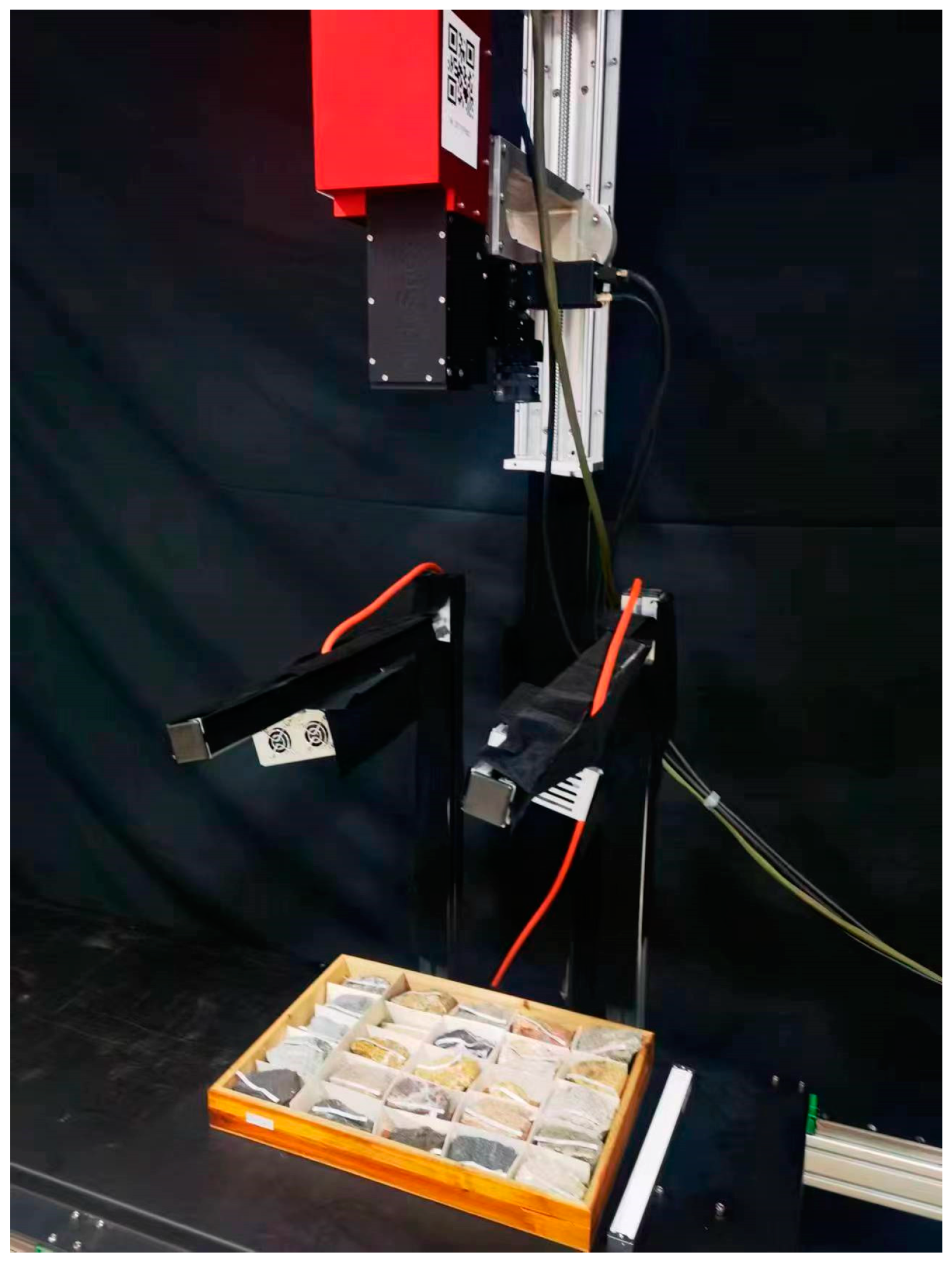
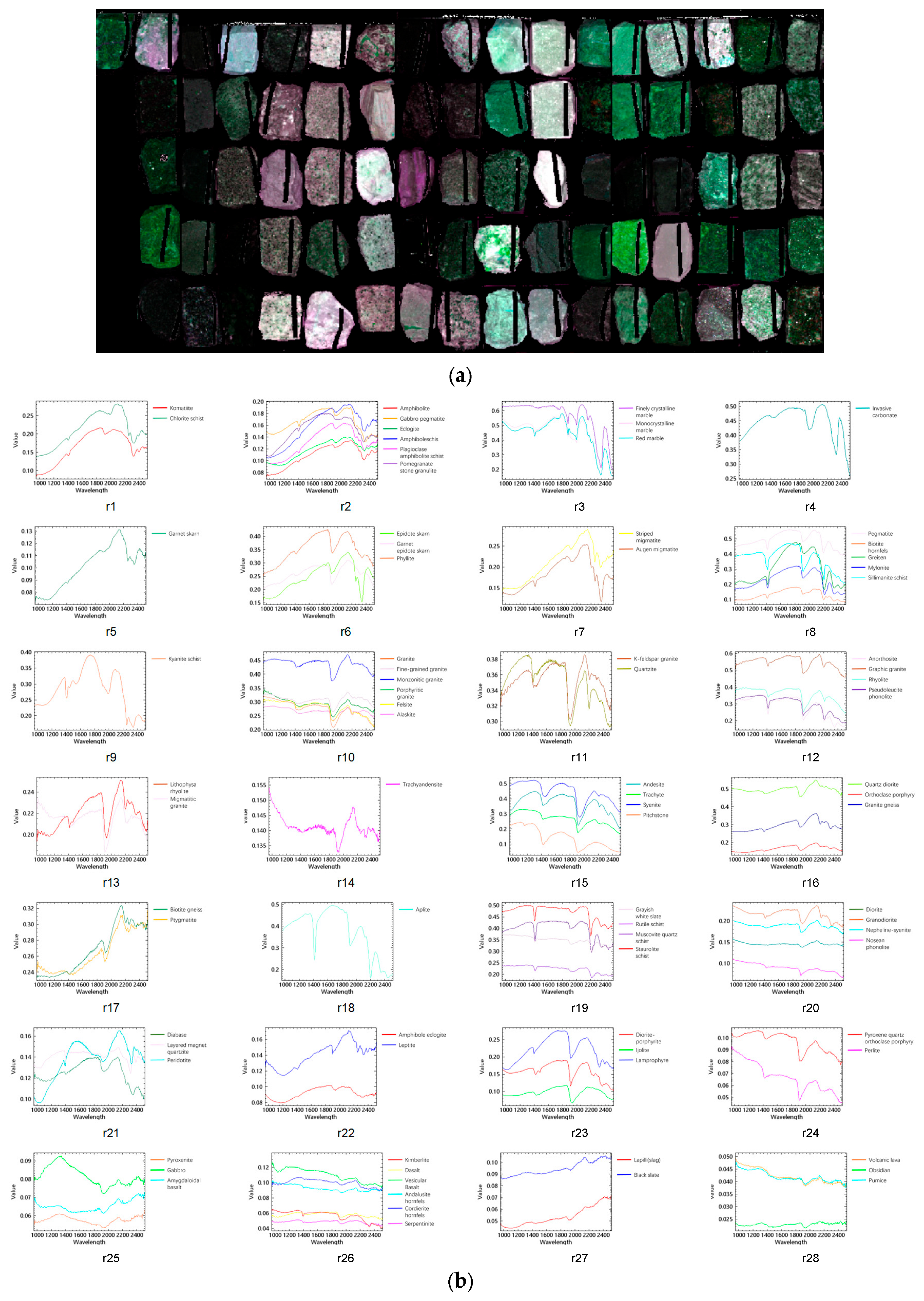
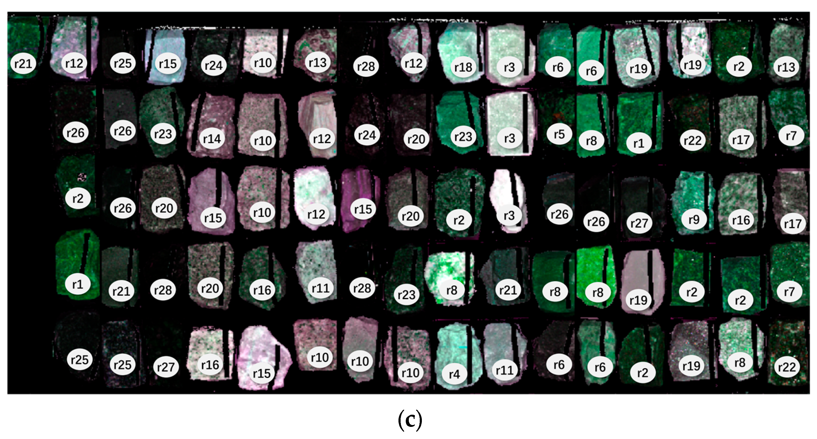
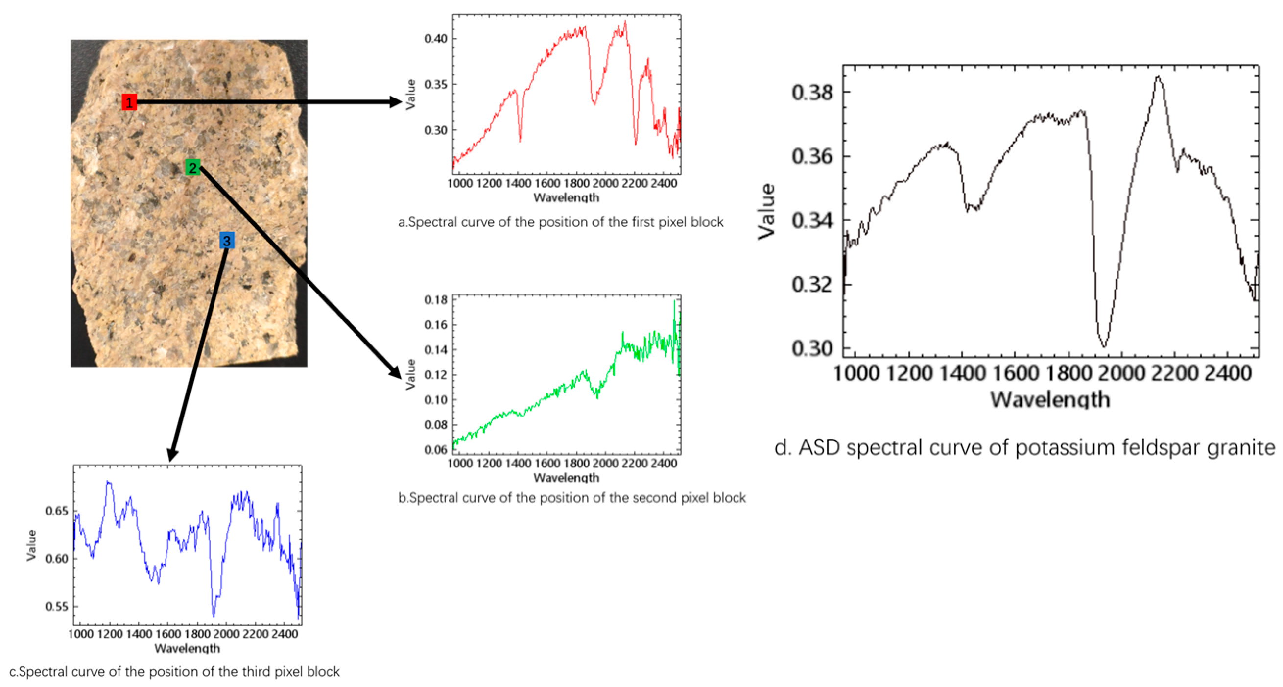
2.1. Rock Dataset
2.2. Methods
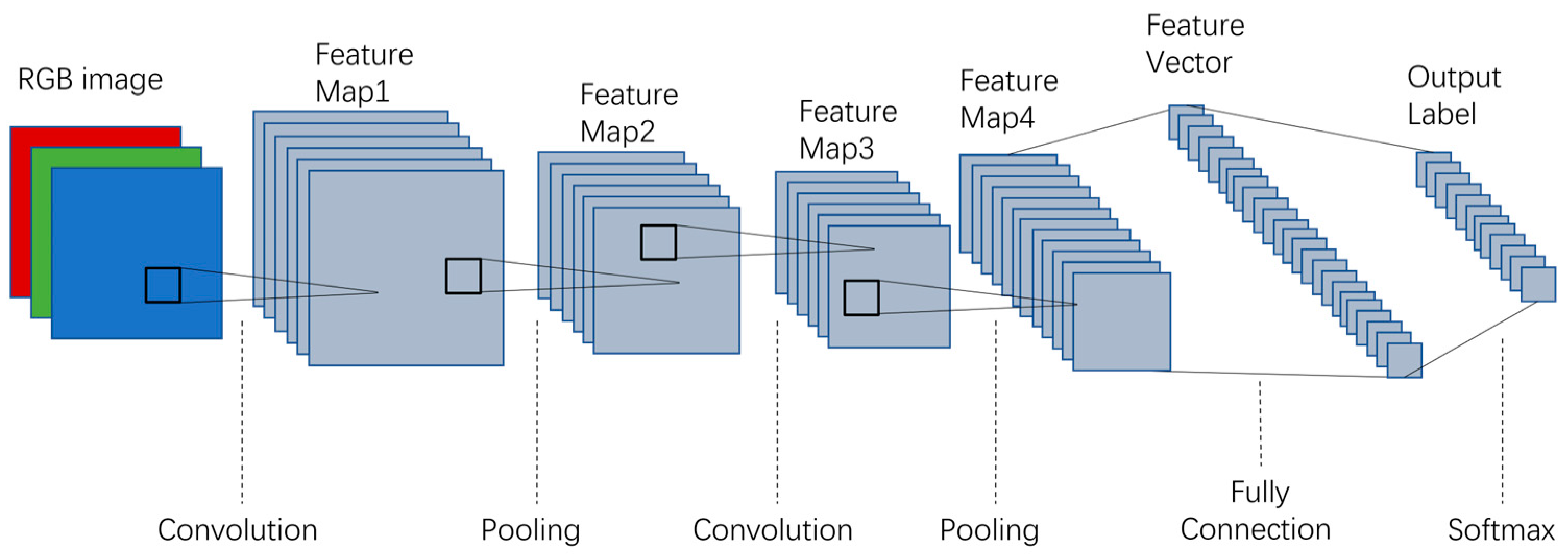
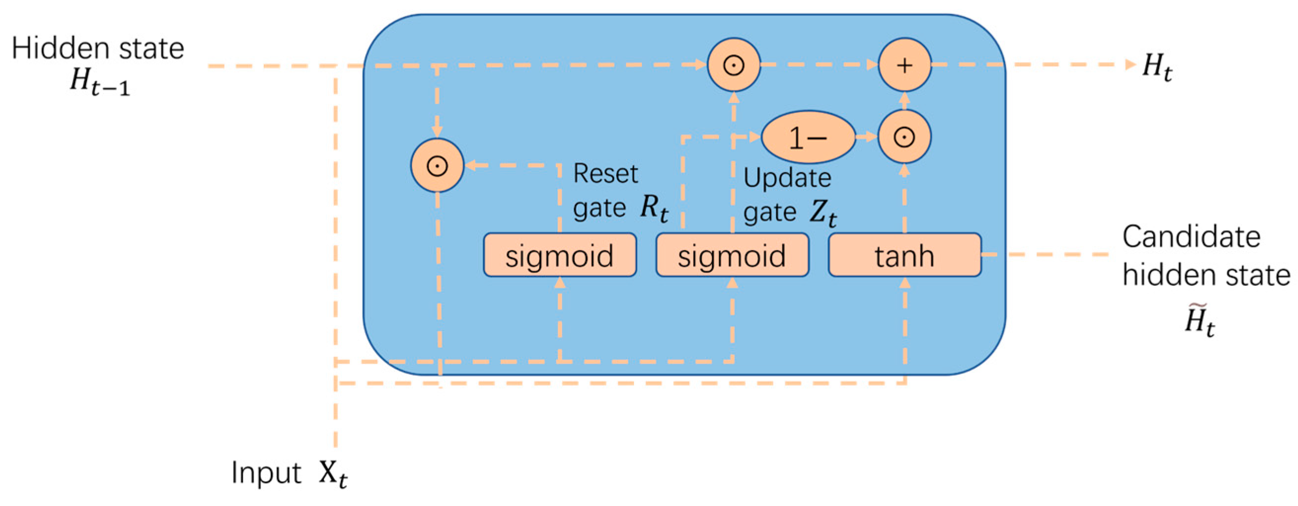
2.2.1. Related Work
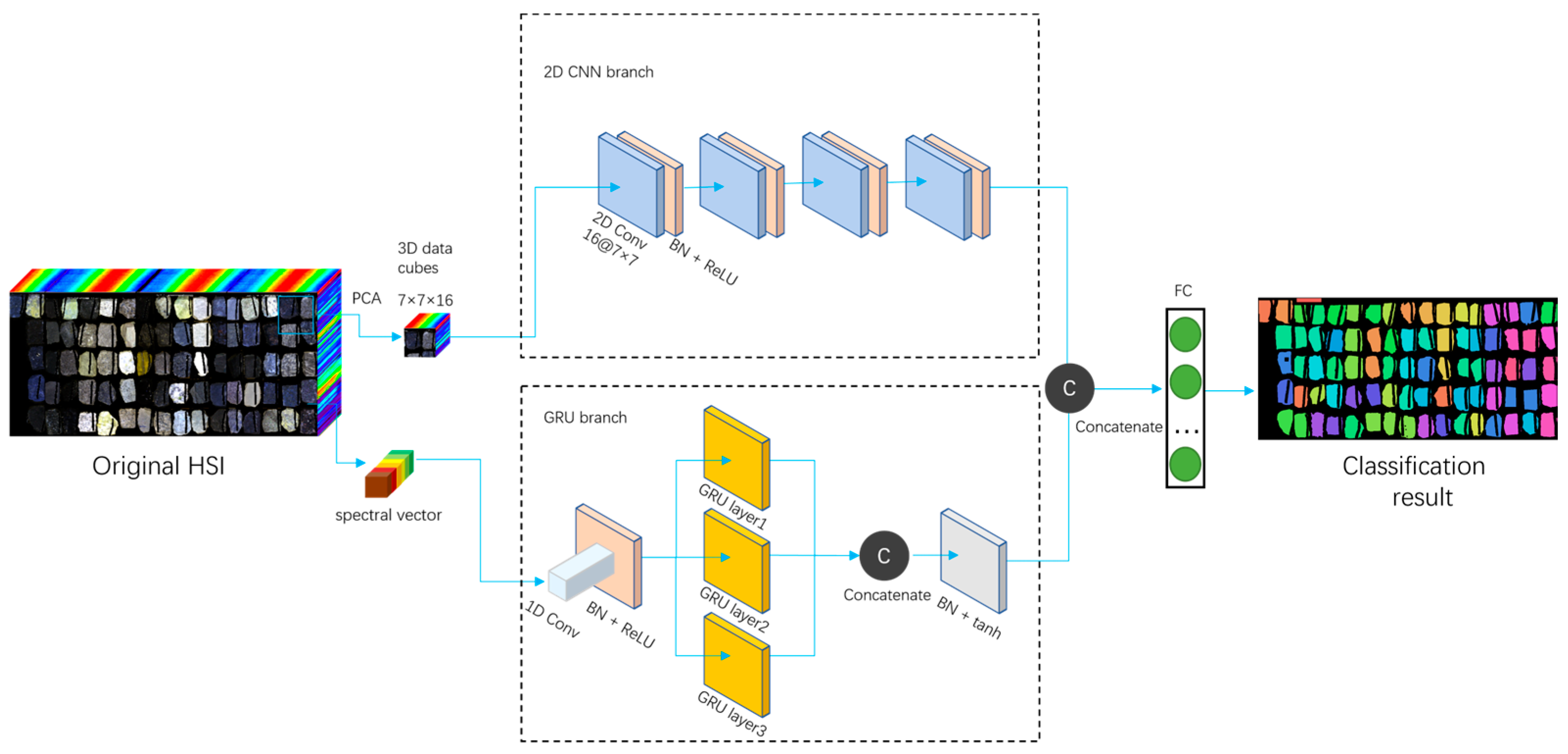
2.2.2. Proposed Method
3. Experiments and Discussion
3.1. Experiment
3.1.1. Experimental Environment and Evaluation Metric
3.1.2. Selection of the Network Backbone
3.1.3. Parameter Settings
3.1.4. Analysis of the Impact of PCA-Preserved Components
3.2. Results and Discussion
4. Conclusions
Author Contributions
Funding
Data Availability Statement
Conflicts of Interest
References
- Jia, J.; Wang, Y.; Chen, J.; Guo, R.; Shu, R.; Wang, J. Status and application of advanced airborne hyperspectral imaging technology: A review. Infrared Phys. Technol. 2020, 104, 103115. [Google Scholar] [CrossRef]
- Bedini, E. The use of hyperspectral remote sensing for mineral exploration: A review. J. Hyperspectral Remote Sens. 2017, 7, 189–211. [Google Scholar] [CrossRef]
- Krupnik, D.; Khan, S. Close-range, ground-based hyperspectral imaging for mining applications at various scales: Review and case studies. Earth-Sci. Rev. 2019, 198, 102952. [Google Scholar] [CrossRef]
- Tripathi, P.; Garg, R.D. Potential of DESIS and PRISMA hyperspectral remote sensing data in rock classification and mineral identification:a case study for Banswara in Rajasthan, India. Environ. Monit. Assess. 2023, 195, 575. [Google Scholar] [CrossRef]
- Monteiro, S.T.; Murphy, R.J.; Ramos, F.; Nieto, J. Applying boosting for hyperspectral classification of ore-bearing rocks. In Proceedings of the 2009 IEEE International Workshop on Machine Learning for Signal Processing, Grenoble, France, 1–4 September 2009; pp. 1–6. [Google Scholar]
- Kokaly, R.F.; Graham, G.E.; Hoefen, T.M.; Kelley, K.D.; Johnson, M.R.; Hubbard, B.E.; Buchhorn, M.; Prakash, A. Multiscale hyperspectral imaging of the Orange Hill Porphyry Copper Deposit, Alaska, USA, with laboratory-, field-, and aircraft-based imaging spectrometers. Proc. Explor. 2017, 17, 923–943. [Google Scholar]
- Wei, J.; Liu, X.; Liu, J. Integrating Textural and Spectral Features to Classify Silicate-Bearing Rocks Using Landsat 8 Data. Appl. Sci. 2016, 6, 283. [Google Scholar] [CrossRef]
- Dkhala, B.; Mezned, N.; Gomez, C.; Abdeljaouad, S. Hyperspectral field spectroscopy and SENTINEL-2 Multispectral data for minerals with high pollution potential content estimation and mapping. Sci. Total Environ. 2020, 740, 140160. [Google Scholar] [CrossRef] [PubMed]
- Kovacevic, M.; Bajat, B.; Trivic, B.; Pavlovic, R. Geological units classification of multispectral images by using support vector machines. In Proceedings of the 2009 International Conference on Intelligent Networking and Collaborative Systems, Barcelona, Spain, 4–6 November 2009; pp. 267–272. [Google Scholar] [CrossRef]
- Lobo, A.; Garcia, E.; Barroso, G.; Martí, D.; Fernandez-Turiel, J.-L.; Ibáñez-Insa, J. Machine Learning for Mineral Identification and Ore Estimation from Hyperspectral Imagery in Tin–Tungsten Deposits: Simulation under Indoor Conditions. Remote Sens. 2021, 13, 3258. [Google Scholar] [CrossRef]
- Buzzi, J.; Riaza, A.; García-Meléndez, E.; Weide, S.; Bachmann, M. Mapping Changes in a Recovering Mine Site with Hyperspectral Airborne HyMap Imagery (Sotiel, SW Spain). Minerals 2014, 4, 313–329. [Google Scholar] [CrossRef]
- Tripathi, M.K.; Govil, H. Evaluation of AVIRIS-NG hyperspectral images for mineral identification and mapping. Heliyon 2019, 5, e02931. [Google Scholar] [CrossRef]
- Hussain, M.; Bird, J.J.; Faria, D.R. A study on CNN transfer learning for image classification. In Proceedings of the Advances in Computational Intelligence Systems: Contributions Presented at the 18th UK Workshop on Computational Intelligence, Nottingham, UK, 5–7 September 2018; pp. 191–202. [Google Scholar]
- Hochreiter, S.; Schmidhuber, J. Long short-term memory. Neural Comput. 1997, 9, 1735–1780. [Google Scholar] [CrossRef] [PubMed]
- López, A.J.; Ramil, A.; Pozo-Antonio, J.S.; Fiorucci, M.P.; Rivas, T. Automatic Identification of Rock-Forming Minerals in Granite Using Laboratory Scale Hyperspectral Reflectance Imaging and Artificial Neural Networks. J. Nondestruct. Eval. 2017, 36, 52. [Google Scholar] [CrossRef]
- Xie, B.; Wu, L.; Mao, W.; Zhou, S.; Liu, S. An Open Integrated Rock Spectral Library (RockSL) for a Global Sharing and Matching Service. Minerals 2022, 12, 118. [Google Scholar] [CrossRef]
- Cardoso-Fernandes, J.; Silva, J.; Dias, F.; Lima, A.; Teodoro, A.C.; Barrès, O.; Cauzid, J.; Perrotta, M.; Roda-Robles, E.; Ribeiro, M.A. Tools for Remote Exploration: A Lithium (Li) Dedicated Spectral Library of the Fregeneda–Almendra Aplite–Pegmatite Field. Data 2021, 6, 33. [Google Scholar] [CrossRef]
- Schneider, S.; Murphy, R.J.; Monteiro, S.T.; Nettleton, E. On the development of a hyperspectral library for autonomous mining systems. In Proceedings of the Australiasian Conference on Robotics and Automation, Sydney, Australia, 2–4 December 2009. [Google Scholar]
- Okyay, Ü.; Khan, S.; Lakshmikantha, M.; Sarmiento, S. Ground-Based Hyperspectral Image Analysis of the Lower Mississippian (Osagean) Reeds Spring Formation Rocks in Southwestern Missouri. Remote Sens. 2016, 8, 1018. [Google Scholar] [CrossRef]
- Douglas, A.; Kereszturi, G.; Schaefer, L.N.; Kennedy, B. Rock alteration mapping in and around fossil shallow intrusions at Mt. Ruapehu New Zealand with laboratory and aerial hyperspectral imaging. J. Volcanol. Geotherm. Res. 2022, 432, 107700. [Google Scholar] [CrossRef]
- Guo, S.; Jiang, Q. Improving Rock Classification with 1D Discrete Wavelet Transform Based on Laboratory Reflectance Spectra and Gaofen-5 Hyperspectral Data. Remote Sens. 2023, 15, 5334. [Google Scholar] [CrossRef]
- Gendrin, A.; Langevin, Y.; Bibring, J.P.; Forni, O. A new method to investigate hyperspectral image cubes: An application of the wavelet transform. J. Geophys. Res. Planets 2006, 111. [Google Scholar] [CrossRef]
- Galdames, F.J.; Perez, C.A.; Estévez, P.A.; Adams, M. Rock lithological instance classification by hyperspectral images using dimensionality reduction and deep learning. Chemom. Intell. Lab. Syst. 2022, 224, 104538. [Google Scholar] [CrossRef]
- He, K.; Gkioxari, G.; Dollár, P.; Girshick, R. Mask r-cnn. In Proceedings of the IEEE International Conference on Computer Vision, Venice, Italy, 22 October 2017; pp. 2961–2969. [Google Scholar]
- Hamedianfar, A.; Laakso, K.; Middleton, M.; Törmänen, T.; Köykkä, J.; Torppa, J. Leveraging High-Resolution Long-Wave Infrared Hyperspectral Laboratory Imaging Data for Mineral Identification Using Machine Learning Methods. Remote Sens. 2023, 15, 4806. [Google Scholar] [CrossRef]
- Abdolmaleki, M.; Consens, M.; Esmaeili, K. Ore-Waste Discrimination Using Supervised and Unsupervised Classification of Hyperspectral Images. Remote Sens. 2022, 14, 6386. [Google Scholar] [CrossRef]
- Fang, Y.; Xiao, Y.; Liang, S.; Ji, Y.; Chen, H. Lithological classification by PCA-QPSO-LSSVM method with thermal infrared hyper-spectral data. J. Appl. Remote Sens. 2022, 16, 044515. [Google Scholar] [CrossRef]
- Xu, Y.; Ma, H.; Peng, S. Study on identification of altered rock in hyperspectral imagery using spectrum of field object. Ore Geol. Rev. 2014, 56, 584–595. [Google Scholar] [CrossRef]
- Ghezelbash, R.; Maghsoudi, A.; Shamekhi, M.; Pradhan, B.; Daviran, M. Genetic algorithm to optimize the SVM and K-means algorithms for mapping of mineral prospectivity. Neural Comput. Appl. 2022, 35, 719–733. [Google Scholar] [CrossRef]
- Bahrambeygi, B.; Moeinzadeh, H. Comparison of support vector machine and neutral network classification method in hyperspectral mapping of ophiolite mélanges—A case study of east of Iran. Egypt. J. Remote Sens. Space Sci. 2017, 20, 1–10. [Google Scholar] [CrossRef]
- Zhang, C.; Yi, M.; Ye, F.; Xu, Q.; Li, X.; Gan, Q. Application and Evaluation of Deep Neural Networks for Airborne Hyperspectral Remote Sensing Mineral Mapping: A Case Study of the Baiyanghe Uranium Deposit in Northwestern Xinjiang, China. Remote Sens. 2022, 14, 5122. [Google Scholar] [CrossRef]
- Miao, Y.; Wu, W.-Y.; Hu, C.-H.; Xu, L.-X.; Fu, X.-H.; Lang, X.-Y.; He, B.-W.; Qian, J.-F. Rock and mineral image dataset based on HySpex hyperspectral imaging system. J. Hangzhou Norm. Univ. (Nat. Sci. Ed.) 2023, 22, 203–210, (In Chinese with English Abstract). [Google Scholar] [CrossRef]
- Hu, C.-H.; Wu, W.-Y.; Miao, Y.; Xu, L.-X.; Fu, X.-H.; Lang, X.-Y.; He, B.-W.; Qian, J.-F. Study on Hyperspectral Rock Classification Based on Initial Rock Classification System. Spectrosc. Spectr. Anal. 2024, 44, 784–792, (In Chinese with English Abstract). [Google Scholar]
- Li, Y.; Zhang, Y.; Huang, X.; Ma, J. Learning Source-Invariant Deep Hashing Convolutional Neural Networks for Cross-Source Remote Sensing Image Retrieval. IEEE Trans. Geosci. Remote Sens. 2018, 56, 6521–6536. [Google Scholar] [CrossRef]
- Makantasis, K.; Karantzalos, K.; Doulamis, A.; Doulamis, N. Deep supervised learning for hyperspectral data classification through convolutional neural networks. In Proceedings of the 2015 IEEE International Geoscience and Remote Sensing Symposium (IGARSS), Milan, Italy, 26–31 July 2015; pp. 4959–4962. [Google Scholar]
- Ma, X.; Dai, Z.; He, Z.; Ma, J.; Wang, Y.; Wang, Y. Learning Traffic as Images: A Deep Convolutional Neural Network for Large-Scale Transportation Network Speed Prediction. Sensors 2017, 17, 818. [Google Scholar] [CrossRef]
- Chung, J.; Gulcehre, C.; Cho, K.; Bengio, Y. Empirical evaluation of gated recurrent neural networks on sequence modeling. arXiv 2014, arXiv:1412.3555. [Google Scholar]
- Mou, L.; Ghamisi, P.; Zhu, X.X. Deep Recurrent Neural Networks for Hyperspectral Image Classification. IEEE Trans. Geosci. Remote Sens. 2017, 55, 3639–3655. [Google Scholar] [CrossRef]
- He, K.; Zhang, X.; Ren, S.; Sun, J. Deep residual learning for image recognition. In Proceedings of the IEEE Conference on Computer Vision and Pattern Recognition, Las Vegas, NV, USA, 27–30 June 2016; pp. 770–778. [Google Scholar]
- Li, Y.; Zhang, H.; Shen, Q. Spectral–Spatial Classification of Hyperspectral Imagery with 3D Convolutional Neural Network. Remote Sens. 2017, 9, 67. [Google Scholar] [CrossRef]
- Ben Hamida, A.; Benoit, A.; Lambert, P.; Ben Amar, C. 3-D Deep Learning Approach for Remote Sensing Image Classification. IEEE Trans. Geosci. Remote Sens. 2018, 56, 4420–4434. [Google Scholar] [CrossRef]
- Roy, S.K.; Krishna, G.; Dubey, S.R.; Chaudhuri, B.B. HybridSN: Exploring 3-D–2-D CNN Feature Hierarchy for Hyperspectral Image Classification. IEEE Geosci. Remote Sens. Lett. 2020, 17, 277–281. [Google Scholar] [CrossRef]
- Deng, Y.; Deng, Y. A Method of SAR Image Automatic Target Recognition Based on Convolution Auto-Encode and Support Vector Machine. Remote Sens. 2022, 14, 5559. [Google Scholar] [CrossRef]


| Class Name | Rock Name | Class Name | Rock Name |
|---|---|---|---|
| r1 | komatiite, chlorite schist | r15 | andesite, trachyte, syenite, pitchstone |
| r2 | garnet granulite, amphibolite, gabbro pegmatite, eclogite, amphiboleschis, plagioclase amphibole schist | r16 | quartz diorite, orthoclase porphyry, granitic gneiss |
| r3 | finely crystalline marble, mesocrystalline marble, red marble | r17 | biotite gneiss, ptygmatite |
| r4 | intrusive carbonate | r18 | aplite |
| r5 | garnet skarn | r19 | grayish white slate, rutile schist, muscovite quartz schist, staurolite schist |
| r6 | epidote skarn, garnet epidote skarn, phyllite | r20 | diorite, granodiorite, nepheline-syenite, nosean phonolite |
| r7 | striped migmatite, augen migmatite | r21 | peridotite, diabase, layered magnet quartzite |
| r8 | pegmatite, biotite hornfels, greisen, mylonite, sillimanite schist | r22 | amphibole eclogite, leptite |
| r9 | kyanite schist | r23 | diorite porphyrite, ijolite, lamprophyre |
| r10 | granite, fine-grained granite, monzonitic granite, porphyritic granite, felsite, alaskite | r24 | pyroxene quartz orthoclase porphyry, perlite |
| r11 | k-feldspar granite, quartzite | r25 | pyroxenite, gabbro, amygdaloidal basalt |
| r12 | anorthosite, graphic granite, rhyolite, pseudoleucite phonolite | r26 | kimberlite, basalt, vesicular basalt, andalusite hornfels, cordierite hornfels, serpentine |
| r13 | lithophysa rhyolite, migmatitic granite | r27 | lapilli (slag), black slate |
| r14 | trachyandesite | r28 | volcanic lava, obsidian, pumice |
| Class | Samples | Class | Samples | Class | Samples | Class | Samples |
|---|---|---|---|---|---|---|---|
r1  | 11,415 | r8  | 22,042 | r15  | 19,547 | r22  | 10,746 |
r2  | 30,779 | r9  | 4718 | r16  | 14,048 | r23  | 14,108 |
r3  | 14,473 | r10  | 30,620 | r17  | 10,351 | r24  | 9242 |
r4  | 5121 | r11  | 9534 | r18  | 5033 | r25  | 14,145 |
r5  | 4434 | r12  | 19,353 | r19  | 19,531 | r26  | 26,830 |
r6  | 11,490 | r13  | 9590 | r20  | 21,145 | r27  | 10,381 |
r7  | 11,129 | r14  | 5471 | r21  | 13,703 | r28  | 11,259 |
| TOTAL | 390,238 | ||||||
| Model | OA (%) | AA (%) | Kappa × 100 |
|---|---|---|---|
| 2-D CNN | 84.011 ± 6.751 | 82.615 ± 7.349 | 83.30 ± 7.1 |
| GRU | 84.610 ± 2.253 | 83.522 ± 2.666 | 83.90 ± 2.4 |
| 2-D CNN-GRU | 97.925 ± 2.831 | 97.956 ± 2.915 | 97.80 ± 3.0 |
| Neighboring Pixel Block Size | Batch Size | ||
|---|---|---|---|
| 64 | 128 | 256 | |
| 5 × 5 | 96.451 | 95.328 | 95.986 |
| 7 × 7 | 96.894 | 97.543 | 97.325 |
| 9 × 9 | 97.145 | 97.249 | 96.874 |
| Retained Components | OA (%) | AA (%) | Kappa × 100 | Average Training Duration (s) |
|---|---|---|---|---|
| 4 | 89.802 ± 4.173 | 88.043 ± 5.922 | 89.00 ± 5.3 | 1698.775 |
| 16 | 97.925 ± 2.831 | 97.956 ± 2.915 | 97.80 ± 3.0 | 1764.083 |
| 32 | 93.119 ± 3.598 | 92.264 ± 6.744 | 92.60 ± 4.4 | 1852.693 |
| 288 | 92.563 ± 2.970 | 93.295 ± 2.642 | 92.20 ± 3.1 | 2023.253 |
| Method | OA (%) | AA (%) | Kappa × 100 |
|---|---|---|---|
| Resnet-18 | 87.995 ± 7.486 | 85.678 ± 8.526 | 87.40 ± 7.8 |
| 3-D CNN | 94.075 ± 3.286 | 92.505 ± 3.717 | 93.80 ± 3.4 |
| Hamida | 88.441 ± 6.411 | 88.003 ± 6.324 | 87.90 ± 6.7 |
| HybridSN | 90.010 ± 2.212 | 89.078 ± 2.469 | 89.50 ± 2.3 |
| CAE-SVM | 91.969 ± 2.798 | 92.228 ± 2.065 | 91.60 ± 2.9 |
| Ours | 97.925 ± 2.831 | 97.956 ± 2.915 | 97.80 ± 3.0 |
| Class Name | Resnet-18 | 3-D CNN | Hamida | HybridSN | CAE-SVM | Ours |
|---|---|---|---|---|---|---|
| r1 | 89.2 ± 10.4 | 97.6 ± 3.4 | 93.0 ± 4.5 | 96.0 ± 4.3 | 94.1 ± 3.8 | 98.6 ± 1.9 |
| r2 | 88.8 ± 5.7 | 94.2 ± 5.9 | 93.1 ± 2.3 | 94.9 ± 3.3 | 95.1 ± 1.6 | 98.8 ± 1.6 |
| r3 | 99.9 ± 0.1 | 99.0 ± 1.1 | 99.2 ± 1.5 | 99.9 ± 0.2 | 95.9 ± 4.7 | 83.8 ± 32.4 |
| r4 | 99.8 ± 0.2 | 99.3 ± 0.5 | 89.3 ± 21.2 | 99.8 ± 0.2 | 90.9 ± 10.4 | 94.1 ± 11.5 |
| r5 | 92.1 ± 5.4 | 95.9 ± 2.3 | 81.0 ± 13.9 | 89.0 ± 7.9 | 76.3 ± 15.3 | 99.2 ± 0.6 |
| r6 | 98.6 ± 1.4 | 98.7 ± 0.6 | 98.8 ± 1.8 | 97.3 ± 1.5 | 97.0 ± 1.6 | 99.5 ± 0.9 |
| r7 | 92.7 ± 2.6 | 92.2 ± 1.7 | 94.4 ± 2.7 | 95.2 ± 1.2 | 90.8 ± 5.0 | 99.4 ± 0.1 |
| r8 | 98.4 ± 1.3 | 97.2 ± 2.3 | 98.5 ± 1.9 | 98.9 ± 0.4 | 97.1 ± 1.5 | 99.9 ± 0.1 |
| r9 | 99.9 ± 0.1 | 99.0 ± 1.2 | 99.8 ± 0.2 | 99.4 ± 0.5 | 97.7 ± 2.0 | 99.4 ± 1.2 |
| r10 | 92.9 ± 2.1 | 96.1 ± 4.1 | 84.9 ± 11.4 | 94.9 ± 2.8 | 94.4 ± 2.9 | 99.5 ± 0.4 |
| r11 | 96.1 ± 2.9 | 98.4 ± 1.1 | 65.9 ± 37.4 | 94.1 ± 3.5 | 94.0 ± 3.0 | 99.8 ± 0.1 |
| r12 | 98.8 ± 0.6 | 97.4 ± 1.8 | 97.8 ± 2.2 | 94.2 ± 1.5 | 95.6 ± 4.3 | 99.8 ± 0.3 |
| r13 | 85.5 ± 3.4 | 88.1 ± 13.9 | 87.1 ± 5.3 | 80.9 ± 5.4 | 83.2 ± 7.1 | 99.5 ± 0.1 |
| r14 | 89.4 ± 6.1 | 97.5 ± 2.8 | 95.3 ± 5.5 | 88.9 ± 8.1 | 90.3 ± 8.1 | 97.5 ± 4.8 |
| r15 | 98.2 ± 2.2 | 98.2 ± 1.7 | 97.5 ± 2.0 | 98.1 ± 1.8 | 96.5 ± 3.0 | 99.5 ± 0.8 |
| r16 | 87.3 ± 5.2 | 98.3 ± 0.8 | 84.7 ± 7.4 | 89.0 ± 4.2 | 93.1 ± 2.2 | 99.3 ± 0.6 |
| r17 | 78.4 ± 20.0 | 94.9 ± 3.3 | 82.8 ± 9.0 | 93.1 ± 2.7 | 93.8 ± 3.8 | 96.7 ± 5.5 |
| r18 | 98.0 ± 0.5 | 95.6 ± 5.7 | 99.6 ± 0.2 | 99.8 ± 0.3 | 94.5 ± 3.7 | 100.0 ± 0.0 |
| r19 | 96.1 ± 1.0 | 94.9 ± 3.4 | 98.4 ± 0.6 | 96.7 ± 4.8 | 97.6 ± 1.8 | 97.9 ± 3.7 |
| r20 | 75.2 ± 12.1 | 96.5 ± 2.3 | 76.0 ± 34.6 | 92.0 ± 4.8 | 94.0 ± 2.4 | 99.4 ± 0.8 |
| r21 | 78.7 ± 17.1 | 96.4 ± 1.1 | 85.1 ± 9.2 | 78.0 ± 12.9 | 86.1 ± 8.0 | 99.5 ± 0.6 |
| r22 | 78.9 ± 11.8 | 88.2 ± 4.0 | 80.2 ± 20.5 | 89.9 ± 5.2 | 90.4 ± 2.3 | 99.1 ± 0.5 |
| r23 | 99.6 ± 0.2 | 98.8 ± 1.5 | 99.0 ± 0.9 | 96.3 ± 1.2 | 98.6 ± 0.6 | 99.9 ± 0.1 |
| r24 | 88.8 ± 2.5 | 93.7 ± 2.8 | 76.6 ± 13.2 | 90.6 ± 2.2 | 86.7 ± 6.8 | 93.9 ± 11.8 |
| r25 | 67.5 ± 10.3 | 91.1 ± 10.3 | 77.0 ± 14.5 | 76.0 ± 9.7 | 91.6 ± 7.0 | 99.4 ± 0.5 |
| r26 | 76.3 ± 9.0 | 90.9 ± 3.0 | 83.5 ± 6.9 | 73.3 ± 9.6 | 88.3 ± 7.1 | 97.6 ± 2.4 |
| r27 | 52.7 ± 10.1 | 87.3 ± 8.0 | 74.2 ± 12.3 | 73.5 ± 9.4 | 74.9 ± 19.7 | 91.9 ± 12.3 |
| r28 | 56.8 ± 6.2 | 53.5 ± 22.1 | 66.8 ± 15.1 | 45.4 ± 11.3 | 78.3 ± 9.8 | 88.1 ± 13.4 |
Disclaimer/Publisher’s Note: The statements, opinions and data contained in all publications are solely those of the individual author(s) and contributor(s) and not of MDPI and/or the editor(s). MDPI and/or the editor(s) disclaim responsibility for any injury to people or property resulting from any ideas, methods, instructions or products referred to in the content. |
© 2024 by the authors. Licensee MDPI, Basel, Switzerland. This article is an open access article distributed under the terms and conditions of the Creative Commons Attribution (CC BY) license (https://creativecommons.org/licenses/by/4.0/).
Share and Cite
Cao, S.; Wu, W.; Wang, X.; Xie, S. Hyperspectral Rock Classification Method Based on Spatial-Spectral Multidimensional Feature Fusion. Minerals 2024, 14, 923. https://doi.org/10.3390/min14090923
Cao S, Wu W, Wang X, Xie S. Hyperspectral Rock Classification Method Based on Spatial-Spectral Multidimensional Feature Fusion. Minerals. 2024; 14(9):923. https://doi.org/10.3390/min14090923
Chicago/Turabian StyleCao, Shixian, Wenyuan Wu, Xinyu Wang, and Shanjuan Xie. 2024. "Hyperspectral Rock Classification Method Based on Spatial-Spectral Multidimensional Feature Fusion" Minerals 14, no. 9: 923. https://doi.org/10.3390/min14090923