
A 3D Geological Modeling Method Using the Transformer Model: A Solution for Sparse Borehole Data

Abstract
1. Introduction
2. Materials and Methods
2.1. Data Preprocessing
- (1)
- Data cleaning: This step checked for errors in each borehole’s data. For example, if the thickness of a stratum was zero, the stratum was removed. Similarly, if the start elevation of a stratum was less than the end elevation of the stratum, it was considered an error, and the stratum was removed.
- (2)
- Data normalization: Considering the large difference in the number of bits between the X and Y coordinates and the elevation, the coordinates were normalized to the range [0, 1]. The normalization formula is shown in Equation (1):
- (3)
- Data encoding: As the stratum name was a character string, a mapping between the string and the integer was created, and the string was encoded as an integer label for processing by the classifier. To prevent data leakage, the preprocessed borehole data were divided into three parts according to the borehole ID, in a specific proportion, to construct the training set, validation set, and test set.
2.2. Construction of KD-Tree
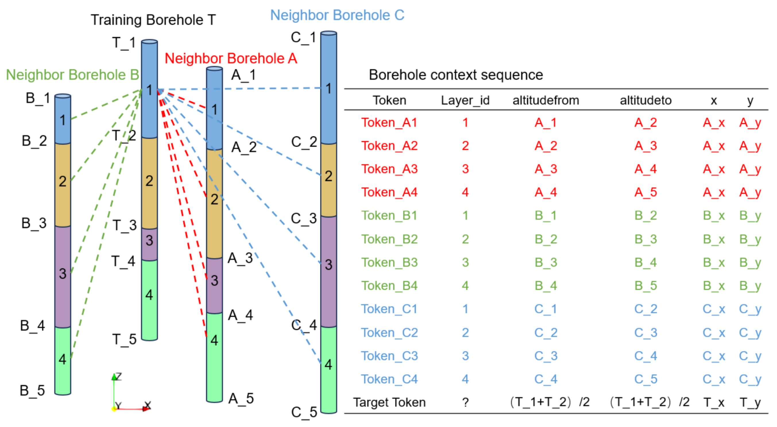
2.3. Construction of Borehole Context Sequence
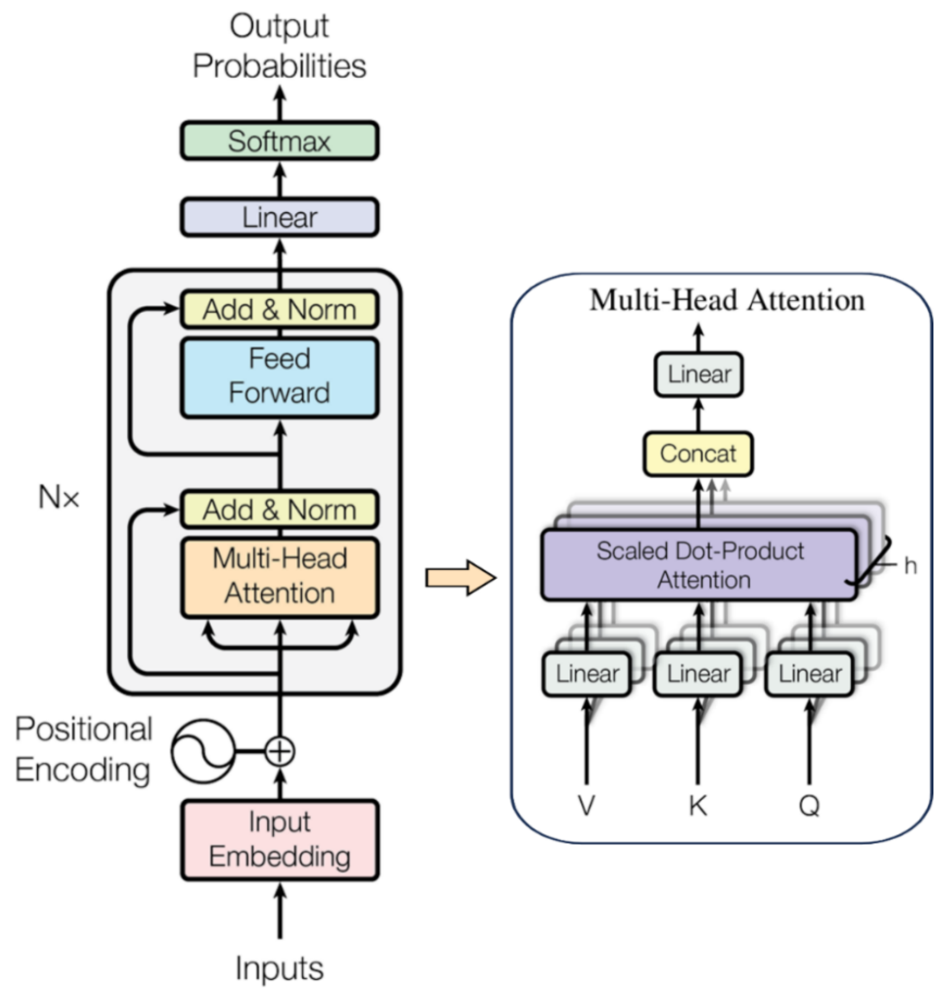
2.4. The Training of the Transformer Model
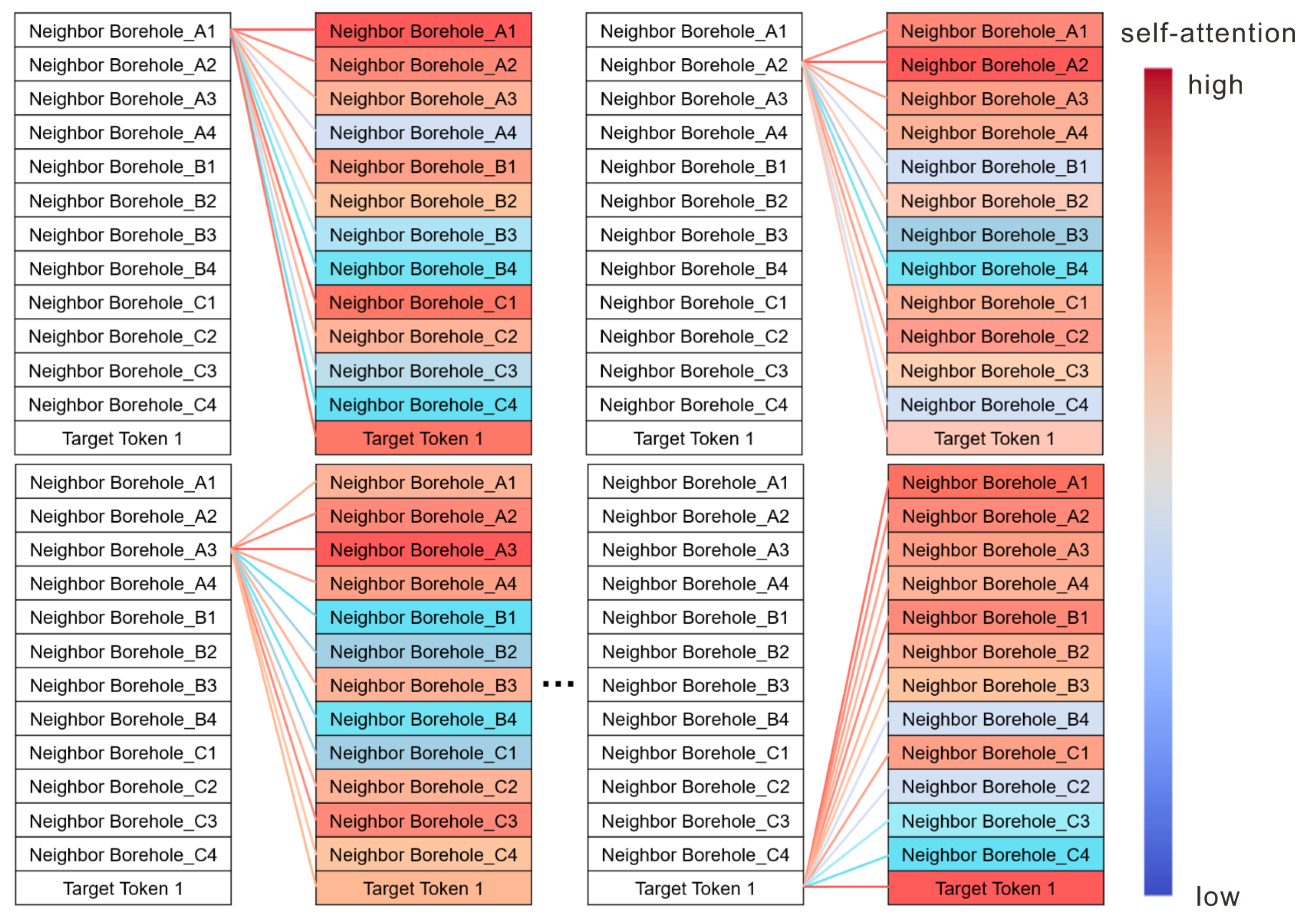
2.5. Model Prediction and Uncertainty Analysis
3. Experiments and Results
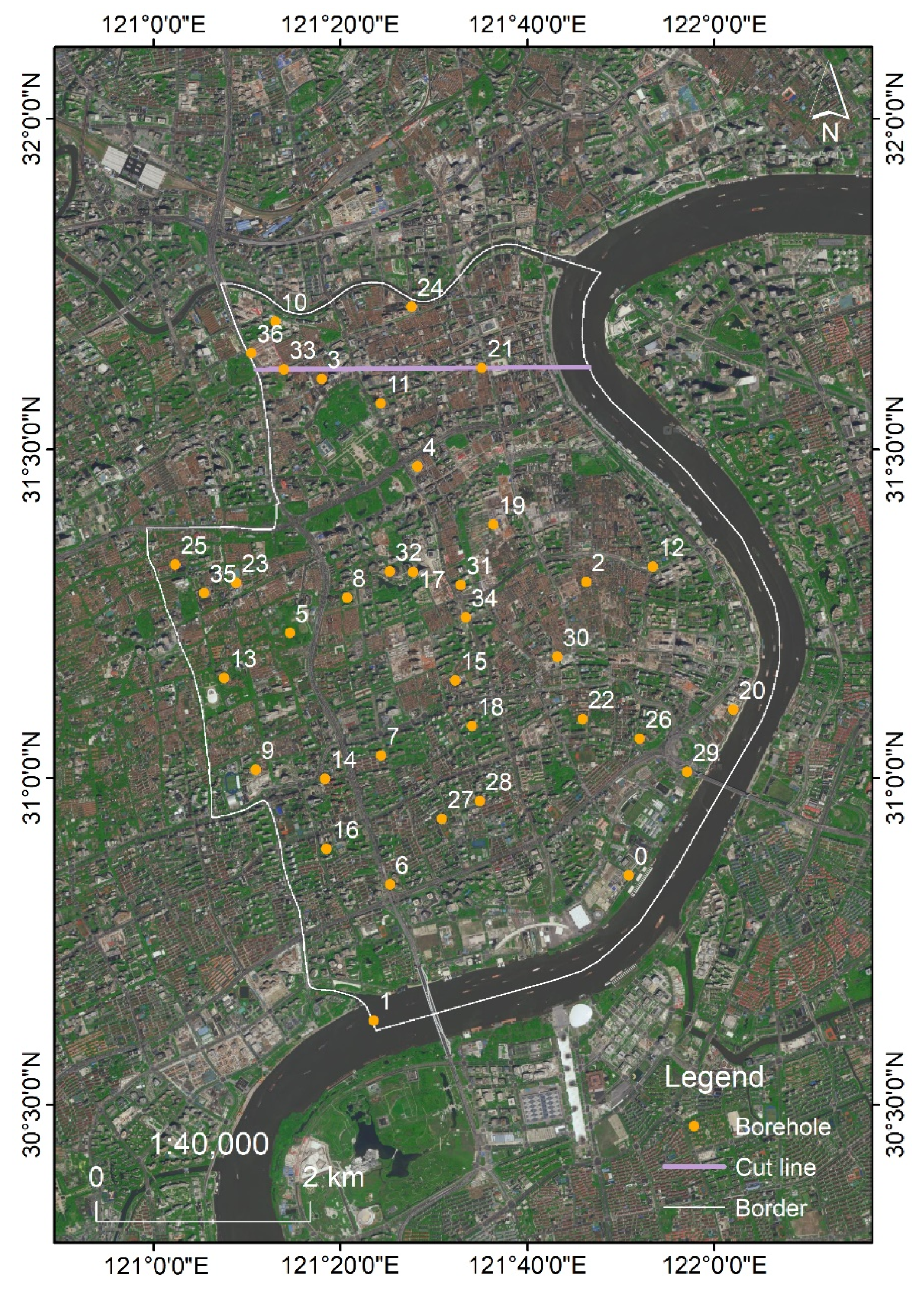
3.1. Experiments
3.2. Results
4. Discussion
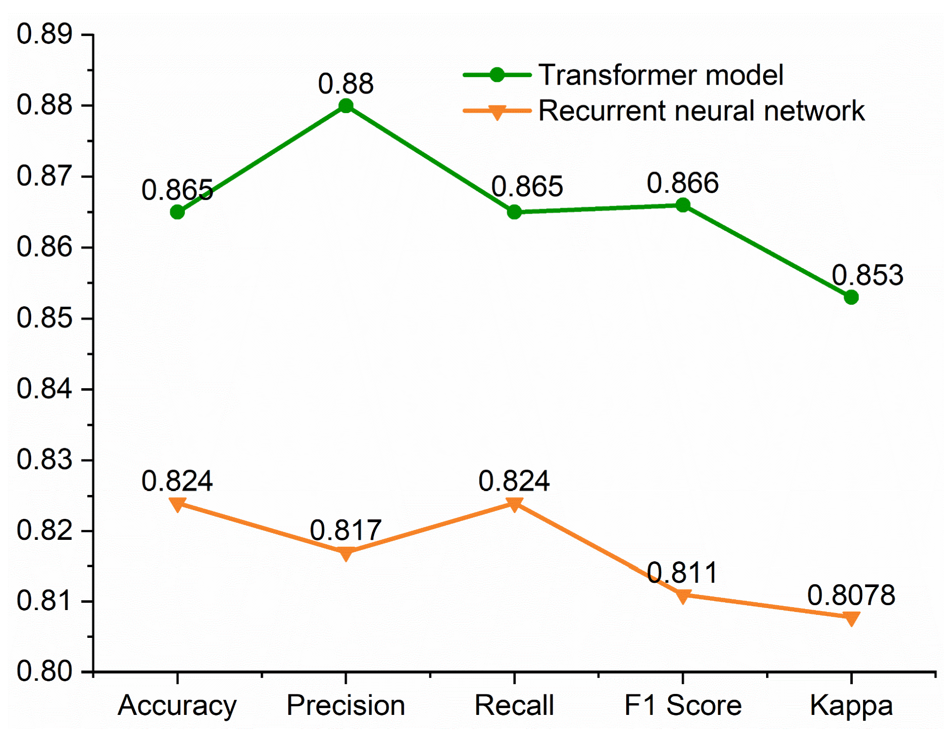
4.1. Comparison of the Transformer Model and Other Methods
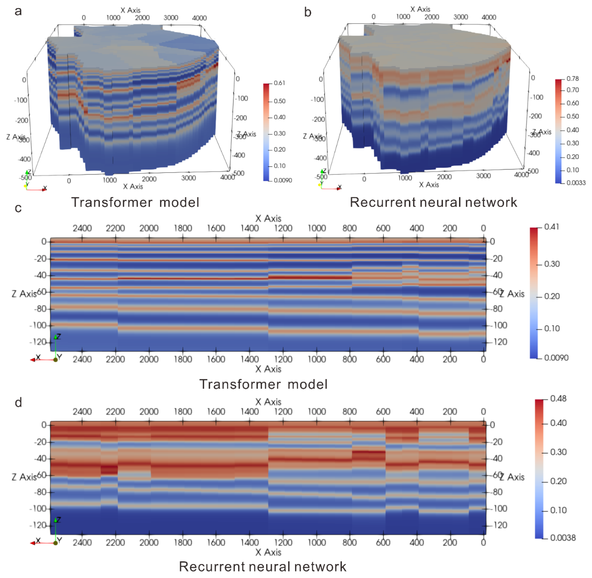
4.2. Analysis of Model Uncertainty
4.3. Advantages and Disadvantages of the Proposed Method
5. Conclusions
Author Contributions
Funding
Data Availability Statement
Acknowledgments
Conflicts of Interest
Abbreviations
| 3D | Three-dimensional |
| KD | K-dimensional |
| IDW | Inverse distance weighting |
| CMC | Coupled Markov chain |
| MRF | Markov random field |
| MPS | Multi-point statistics |
| CNN | Convolutional neural network |
| RNN | Recurrent neural network |
| GAN | Generative adversarial network |
| GPT | Generative pre-trained transformer |
| ID | Identifier |
| ROC | Receiver operating characteristic |
| AUC | Area under the curve |
| RMSE | Root mean square error |
References
- Lyu, M.; Ren, B.; Wu, B.; Tong, D.; Ge, S.; Han, S. A parametric 3D geological modeling method considering stratigraphic interface topology optimization and coding expert knowledge. Eng. Geol. 2021, 293, 106300. [Google Scholar] [CrossRef]
- Zhou, G.; Chen, J.; An, W.; Liu, C.; Li, W. Three-dimensional mineral prospectivity mapping based on natural language processing and random forests: A case study of the Xiyu diamond deposit, China. Ore Geol. Rev. 2024, 169, 106082. [Google Scholar] [CrossRef]
- Ji, G.; Wang, Q.; Zhou, X.; Cai, Z.; Zhu, J.; Lu, Y. An automated method to build 3D multi-scale geological models for engineering sedimentary layers with stratum lenses. Eng. Geol. 2023, 317, 107077. [Google Scholar] [CrossRef]
- Zhu, L.; Zhang, C.; Li, M.; Pan, X.; Sun, J. Building 3D solid models of sedimentary stratigraphic systems from borehole data: An automatic method and case studies. Eng. Geol. 2011, 127, 1–13. [Google Scholar] [CrossRef]
- Yeh, C.H.; Lu, Y.C.; Khoshnevisan, S.; Juang, C.H.; Tien, Y.M.; Dong, J.Y. LiDAR-based 3D litho-stratigraphic models calibrated with limited boreholes. Engineering Geology. 2024, 332. [Google Scholar] [CrossRef]
- Chen, G.; Zhu, J.; Qiang, M.; Gong, W. Three-dimensional site characterization with borehole data—A case study of Suzhou area. Eng. Geol. 2018, 234, 65–82. [Google Scholar] [CrossRef]
- Qiu, Y.; Zhang, N.; Yin, Z.; Wang, Y.; Xu, C.; Zhang, P. Novel multi-spatial receptive field (MSRF) XGBoost method for predicting geological cross-section based on sparse borehole data. Eng. Geol. 2024, 338, 107604. [Google Scholar] [CrossRef]
- Lyu, B.; Wang, Y.; Shi, C. Multi-scale generative adversarial networks (GAN) for generation of three-dimensional subsurface geological models from limited boreholes and prior geological knowledge. Comput. Geotech. 2024, 170, 106336. [Google Scholar] [CrossRef]
- Hou, W.; Yang, L.; Deng, D.; Ye, J.; Clarke, K.; Yang, Z.; Zhuang, W.; Liu, J.; Huang, J. Assessing quality of urban underground spaces by coupling 3D geological models: The case study of Foshan city, South China. Comput. Geosci. 2016, 89, 1–11. [Google Scholar] [CrossRef]
- Kessler, H.; Mathers, S.; Sobisch, H.-G. The capture and dissemination of integrated 3D geospatial knowledge at the British Geological Survey using GSI3D software and methodology. Comput. Geosci. 2009, 35, 1311–1321. [Google Scholar] [CrossRef]
- Wang, J.; Zhao, H.; Bi, L.; Wang, L. Implicit 3D Modeling of Ore Body from Geological Boreholes Data Using Hermite Radial Basis Functions. Minerals 2018, 8, 443. [Google Scholar] [CrossRef]
- Jessell, M.; Aillères, L.; De Kemp, E.; Lindsay, M.; Wellmann, F.; Hillier, M.; Laurent, G.; Carmichael, T.; Martin, R. Next Generation Three-Dimensional Geologic Modeling and Inversion. In Proceedings of the SEG Conference on Keystone—Building Exploration Capability for the 21st Century, Keystone, CO, USA, 27–30 September 2014. [Google Scholar]
- Mallet, J.L. Discrete modeling for natural objects. J. Int. Assoc. Math. Geol. 1997, 29, 199–219. [Google Scholar] [CrossRef]
- Liu, H.; Chen, S.; Hou, M.; He, L. Improved inverse distance weighting method application considering spatial autocorrelation in 3D geological modeling. Earth Sci. Informatics 2019, 13, 619–632. [Google Scholar] [CrossRef]
- Jātnieks, J.; Popovs, K.; Saks, T. A comprehensive approach to the 3D geological modelling of sedimentary basins: Example of Latvia, the central part of the Baltic Basin. Estonian J. Earth Sci. 2015, 64, 173–188. [Google Scholar] [CrossRef]
- Calcagno, P.; Chilès, J.P.; Courrioux, G.; Guillen, A. Geological modelling from field data and geological knowledge Part I. Modelling method coupling 3D potential-field interpolation and geological rules. Phys. Earth Planet. Inter. 2008, 171, 147–157. [Google Scholar] [CrossRef]
- von Harten, J.; de la Varga, M.; Hillier, M.; Wellmann, F. Informed Local Smoothing in 3D Implicit Geological Modeling. Minerals 2021, 11, 1281. [Google Scholar] [CrossRef]
- Lu, G.Y.; Wong, D.W. An adaptive inverse-distance weighting spatial interpolation technique. Comput. Geosci. 2008, 34, 1044–1055. [Google Scholar] [CrossRef]
- Zhou, C.; Ouyang, J.; Ming, W.; Zhang, G.; Du, Z.; Liu, Z. A Stratigraphic Prediction Method Based on Machine Learning. Appl. Sci. 2019, 9, 3553. [Google Scholar] [CrossRef]
- Smirnoff, A.; Boisvert, E.; Paradis, S.J. Support vector machine for 3D modelling from sparse geological information of various origins. Comput. Geosci. 2008, 34, 127–143. [Google Scholar] [CrossRef]
- Sun, L.; Wei, Y.; Cai, H.; Yan, J.; Xiao, J. Improved Fast Adaptive IDW Interpolation Algorithm based on the Borehole Data Sample Characteristic and Its Application. J. Physics Conf. Ser. 2019, 1284, 012074. [Google Scholar] [CrossRef]
- Wang, Y.; Akeju, O.V.; Zhao, T. Interpolation of spatially varying but sparsely measured geo-data: A comparative study. Eng. Geol. 2017, 231, 200–217. [Google Scholar] [CrossRef]
- Fouedjio, F.; Scheidt, C.; Yang, L.; Achtziger-Zupančič, P.; Caers, J. A geostatistical implicit modeling framework for uncertainty quantification of 3D geo-domain boundaries: Application to lithological domains from a porphyry copper deposit. Comput. Geosci. 2021, 157, 104931. [Google Scholar] [CrossRef]
- Qi, X.-H.; Li, D.-Q.; Phoon, K.-K.; Cao, Z.-J.; Tang, X.-S. Simulation of geologic uncertainty using coupled Markov chain. Eng. Geol. 2016, 207, 129–140. [Google Scholar] [CrossRef]
- Gong, W.; Zhao, C.; Juang, C.H.; Tang, H.; Wang, H.; Hu, X. Stratigraphic uncertainty modelling with random field approach. Comput. Geotech. 2020, 125, 103681. [Google Scholar] [CrossRef]
- Li, Z.; Wang, X.; Wang, H.; Liang, R.Y. Quantifying stratigraphic uncertainties by stochastic simulation techniques based on Markov random field. Eng. Geol. 2016, 201, 106–122. [Google Scholar] [CrossRef]
- Chen, Q.; Liu, G.; Ma, X.; Li, X.; He, Z. 3D stochastic modeling framework for Quaternary sediments using multiple-point statistics: A case study in Minjiang Estuary area, southeast China. Comput. Geosci. 2020, 136, 104404. [Google Scholar] [CrossRef]
- Zhao, Y.; Chen, J.; Yang, S.; He, K.; Shimada, H.; Sasaoka, T. A Multi-Point Geostatistical Modeling Method Based on 2D Training Image Partition Simulation. Mathematics 2023, 11, 4900. [Google Scholar] [CrossRef]
- Abdollahifard, M.J.; Baharvand, M.; Mariéthoz, G. Efficient training image selection for multiple-point geostatistics via analysis of contours. Comput. Geosci. 2019, 128, 41–50. [Google Scholar] [CrossRef]
- Kim, H.-S.; Ji, Y. Three-dimensional geotechnical-layer mapping in Seoul using borehole database and deep neural network-based model. Eng. Geol. 2022, 297, 106489. [Google Scholar] [CrossRef]
- Guo, J.; Xu, X.; Wang, L.; Wang, X.; Wu, L.; Jessell, M.; Ogarko, V.; Liu, Z.; Zheng, Y. GeoPDNN 1.0: A semi-supervised deep learning neural network using pseudo-labels for three-dimensional shallow strata modelling and uncertainty analysis in urban areas from borehole data. Geosci. Model Dev. 2024, 17, 957–973. [Google Scholar] [CrossRef]
- Bi, Z.; Wu, X.; Li, Z.; Chang, D.; Yong, X. DeepISMNet: Three-dimensional implicit structural modeling with convolutional neural network. Geosci. Model Dev. 2022, 15, 6841–6861. [Google Scholar] [CrossRef]
- Jessell, M.; Guo, J.; Li, Y.; Lindsay, M.; Scalzo, R.; Giraud, J.; Pirot, G.; Cripps, E.; Ogarko, V. Into the Noddyverse: A massive data store of 3D geological models for machine learning and inversion applications. Earth Syst. Sci. Data 2022, 14, 381–392. [Google Scholar] [CrossRef]
- Hillier, M.; Wellmann, F.; Brodaric, B.; de Kemp, E.; Schetselaar, E. Three-Dimensional Structural Geological Modeling Using Graph Neural Networks. Math. Geosci. 2021, 53, 1725–1749. [Google Scholar] [CrossRef]
- Han, S.; Zhang, Y.; Wang, J.; Tong, D.; Lyu, M. Graph neural network-based topological relationships automatic identification of geological boundaries. Comput. Geosci. 2024, 188, 105621. [Google Scholar] [CrossRef]
- Battalgazy, N.; Valenta, R.; Gow, P.; Spier, C.; Forbes, G. Addressing Geological Challenges in Mineral Resource Estimation: A Comparative Study of Deep Learning and Traditional Techniques. Minerals 2023, 13, 982. [Google Scholar] [CrossRef]
- Zhou, Y.Z.; Wang, J.; Zuo, R.G.; Xiao, F.; Shen, W.J.; Wang, S.G. Machine learning, deep learning and Python language in field of geology. Acta Petrologica Sinica. 2018, 34, 3173–3178. [Google Scholar]
- Vaswani, A.; Shazeer, N.; Parmar, N.; Uszkoreit, J.; Jones, L.; Gomez, A.N.; Kaiser, L.; Polosukhin, I. Attention Is All You Need. In Proceedings of the 31st Annual Conference on Neural Information Processing Systems (NIPS), Long Beach, CA, USA, 4–9 December 2017. [Google Scholar]
- Wei, J.; Wang, Z.; Li, Z.; Li, Z.; Pang, S.; Xi, X.; Cribb, M.; Sun, L. Global aerosol retrieval over land from Landsat imagery integrating Transformer and Google Earth Engine. Remote Sens. Environ. 2024, 315, 114404. [Google Scholar] [CrossRef]
- Zhao, Y.; Zhang, J.; Zong, C. Transformer: A General Framework from Machine Translation to Others. Mach. Intell. Res. 2023, 20, 514–538. [Google Scholar] [CrossRef]
- Li, Y.H.; Yao, T.; Pan, Y.W.; Mei, T. Contextual Transformer Networks for Visual Recognition. IEEE Trans. Pattern Anal. Mach. Intell. 2023, 45, 1489–1500. [Google Scholar] [CrossRef]
- Feng, R.; Li, Z.; Liu, B.; Ding, Y. A Joint Spatiotemporal Prediction and Image Confirmation Model for Vehicle Trajectory Concatenation with Low Detection Rates. IEEE Trans. Intell. Transp. Syst. 2024, 25, 11701–11715. [Google Scholar] [CrossRef]
- Tiwari, A.; Singh, R.K.; Shigwan, S.J. SwinDTI: Swin transformer-based generalized fast estimation of diffusion tensor parameters from sparse data. Neural Comput. Appl. 2023, 36, 3179–3196. [Google Scholar] [CrossRef]
- Kakde, H.M. Range Searching Using kd Tree; Florida State University: Tallahassee, FL, USA, 2005. [Google Scholar]
- Anzola, J.; Pascual, J.; Tarazona, G.; Crespo, R.G. A Clustering WSN Routing Protocol Based on k-d Tree Algorithm. Sensors 2018, 18, 2899. [Google Scholar] [CrossRef] [PubMed]
- Tiwari, V.R. Developments in KD tree and KNN searches. Int. J. Comput. Appl. 2023, 975, 8887. [Google Scholar] [CrossRef]
- Castellucci, G.; Bellomaria, V.; Favalli, A.; Romagnoli, R. Multi-lingual intent detection and slot filling in a joint bert-based model. arXiv 2019, arXiv:1907.02884. [Google Scholar]
- Lan, L.; Zhang, Q.; Zhu, W.; Ye, G.; Shi, Y.; Zhu, H. Geotechnical characterization of deep Shanghai clays. Eng. Geol. 2022, 307, 106794. [Google Scholar] [CrossRef]
- Shi, Y.J.; Yan, X.X.; Wang, J.H.; Fang, Z.; Li, B. Evaluation of Engineering Geological Condition in Shanghai Coastal Area. In Proceedings of the International Symposium on Coastal Engineering Geology (ISCEG), Shanghai, China, 20–21 September 2012; Tongji University: Shanghai, China, 2012. [Google Scholar]
- Ray, P.; Le Manach, Y.; Riou, B.; Houle, T.T.; Warner, D.S. Statistical Evaluation of a Biomarker. Anesthesiology 2010, 112, 1023–1040. [Google Scholar] [CrossRef]
- Tian, T.L.; Song, C.; Ting, J.; Huang, H.Y. A French-to-English Machine Translation Model Using Transformer Network. In Proceedings of the 8th International Conference on Information Technology and Quantitative Management (ITQM)—Developing Global Digital Economy after COVID-19, Chengdu, China, 9–11 July 2021. [Google Scholar]
- Huang, Z.; Wang, P.; Wang, J.; Miao, H.; Xu, J.; Zhang, P. Improving Transformer Based End-to-End Code-Switching Speech Recognition Using Language Identification. Appl. Sci. 2021, 11, 9106. [Google Scholar] [CrossRef]
- Yang, Z.; Chen, Q.; Cui, Z.; Liu, G.; Dong, S.; Tian, Y. Automatic reconstruction method of 3D geological models based on deep convolutional generative adversarial networks. Comput. Geosci. 2022, 26, 1135–1150. [Google Scholar] [CrossRef]
- Fan, W.; Liu, G.; Chen, Q.; Cui, Z.; Yang, Z.; Huang, Q.; Wu, X. Geological model automatic reconstruction based on conditioning Wasserstein generative adversarial network with gradient penalty. Earth Sci. Informatics 2023, 16, 2825–2843. [Google Scholar] [CrossRef]
- Castangia, M.; Grajales, L.M.M.; Aliberti, A.; Rossi, C.; Macii, A.; Macii, E.; Patti, E. Transformer neural networks for interpretable flood forecasting. Environ. Model. Softw. 2023, 160, 105581. [Google Scholar] [CrossRef]
- Zhu, L.-F.; Li, M.-J.; Li, C.-L.; Shang, J.-G.; Chen, G.-L.; Zhang, B.; Wang, X.-F. Coupled modeling between geological structure fields and property parameter fields in 3D engineering geological space. Eng. Geol. 2013, 167, 105–116. [Google Scholar] [CrossRef]
- Zhang, Q.; Zhu, H. Collaborative 3D geological modeling analysis based on multi-source data standard. Eng. Geol. 2018, 246, 233–244. [Google Scholar] [CrossRef]


| Modeling Methods | Advantages | Disadvantages | |
|---|---|---|---|
| Deterministic methods | Explicit method | It is convenient for geologists to participate directly and maximize the use of geological knowledge, and the results are controllable. | Time-consuming, laborious, and subjective. |
| Implicit method | High modeling efficiency. | This method cannot best use available data or contain sufficient geological constraints. | |
| Stochastic methods | Coupled Markov chain, Markov random field | This method can generate multiple possible geological models, reflecting the uncertainty of geology. | Using this method it is difficult to determine the transition probability matrix; the reliability depends on experience. |
| Gaussian simulations | Smooth model. | The ability to represent complex geological structures is limited. | |
| Multi-point statistics | This method can capture complex geological models; the generated model is highly consistent with the training image. | At least one training image is needed to represent geological knowledge; the tuning of MPS parameters is also needed. | |
| Machine learning and deep learning | It has strong objectivity, a strong modeling ability for complex nonlinear geological structures, and high modeling efficiency. | High computing power requirements. | |
| Geological Era | Engineering Geological Layer | ||
|---|---|---|---|
| No. | Name | ||
| Holocene | ① | Fill | |
| ② | Brown–yellow silty clay | ||
| ③ | Gray muddy silty clay | ||
| ④ | Gray muddy clay | ||
| ⑤1 | Gray silty clay | ||
| ⑤2 | Gray sandy clay | ||
| ⑤3 | Gray silty clay | ||
| ⑤4 | Gray–green silty clay | ||
| Upper Pleistocene | ⑥ | Dark green–brown–yellow silty clay | |
| ⑦1 | Grass yellow–gray sandy silt | ||
| ⑦2 | Gray yellow–gray powder sand | ||
| ⑧ | Gray silty clay | ||
| ⑨1 | Cyan–gray silty sand | ||
| ⑨2 | Gray gravelly medium sand | ||
| Middle Pleistocene | ⑩ | Blue–gray silty clay | |
| Parameters | Value |
|---|---|
| Training set: validation set: test set | 6:2:2 |
| Embed dims | 256 |
| Num heads | 8 |
| Num layers | 6 |
| Learning rate | |
| Number of training epochs | 500 |
| Loss function | Cross-entropy loss |
| Optimizer | Adam |
| Number of neighbor boreholes (k) | 3 |
| Metric | Value |
|---|---|
| Accuracy | 0.86 |
| Precision | 0.88 |
| Recall | 0.86 |
| F1 Score | 0.86 |
| Kappa Coefficient | 0.85 |
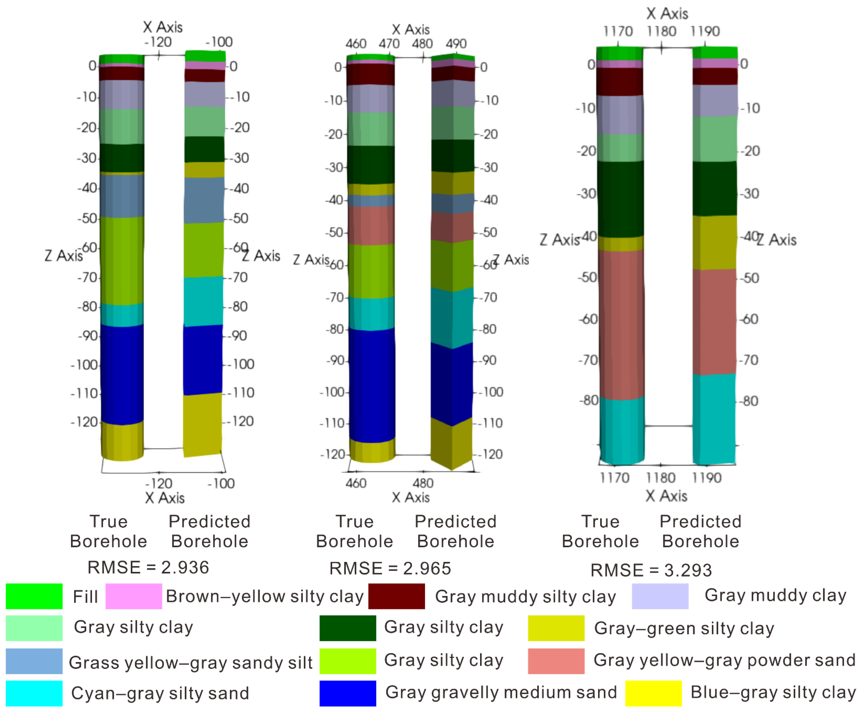
| Borehole ID | RMSE of IDW | RMSE of Kriging | RMSE of Transformer Model |
|---|---|---|---|
| 3 | 4.135 | 3.435 | 2.965 |
| 17 | 4.515 | 3.947 | 3.293 |
| 36 | 4.093 | 3.376 | 2.936 |
| Average | 4.248 | 3.586 | 3.065 |
Disclaimer/Publisher’s Note: The statements, opinions and data contained in all publications are solely those of the individual author(s) and contributor(s) and not of MDPI and/or the editor(s). MDPI and/or the editor(s) disclaim responsibility for any injury to people or property resulting from any ideas, methods, instructions or products referred to in the content. |
© 2025 by the authors. Licensee MDPI, Basel, Switzerland. This article is an open access article distributed under the terms and conditions of the Creative Commons Attribution (CC BY) license (https://creativecommons.org/licenses/by/4.0/).
Share and Cite
Hang, Z.; Xue, T.; Chen, J.; Shi, Y.; Yin, Z.; Cui, Z.; Zhou, G. A 3D Geological Modeling Method Using the Transformer Model: A Solution for Sparse Borehole Data. Minerals 2025, 15, 301. https://doi.org/10.3390/min15030301
Hang Z, Xue T, Chen J, Shi Y, Yin Z, Cui Z, Zhou G. A 3D Geological Modeling Method Using the Transformer Model: A Solution for Sparse Borehole Data. Minerals. 2025; 15(3):301. https://doi.org/10.3390/min15030301
Chicago/Turabian StyleHang, Zhenquan, Tao Xue, Jianping Chen, Yujin Shi, Zehang Yin, Zijia Cui, and Guanyun Zhou. 2025. "A 3D Geological Modeling Method Using the Transformer Model: A Solution for Sparse Borehole Data" Minerals 15, no. 3: 301. https://doi.org/10.3390/min15030301
APA StyleHang, Z., Xue, T., Chen, J., Shi, Y., Yin, Z., Cui, Z., & Zhou, G. (2025). A 3D Geological Modeling Method Using the Transformer Model: A Solution for Sparse Borehole Data. Minerals, 15(3), 301. https://doi.org/10.3390/min15030301