1. Introduction
In the last seventy years, many traffic flow models have been developed and researched. Two of the most commonly used macroscopic models are the celebrated first-order Lighthill–Whitham–Richards (LWR) model, [
1,
2] and the second-order Aw-Rascle–Zhang model [
3,
4]. In both cases, the so-called Fundamental Diagram (FD) provides a closure of the evolution equations, thus allowing a well-posed theory and well-grounded simulation tools (see [
5]). The FD usually refers to the empirically observed flow-occupancy curve, which in mathematical terms refers to the functional relationship between flow and density (modeling counterpart of occupancy) or between average speed of vehicles and density. For macroscopic fluid-dynamic models, there is a rich discussion on FD (see, e.g., [
5,
6,
7,
8,
9,
10]).
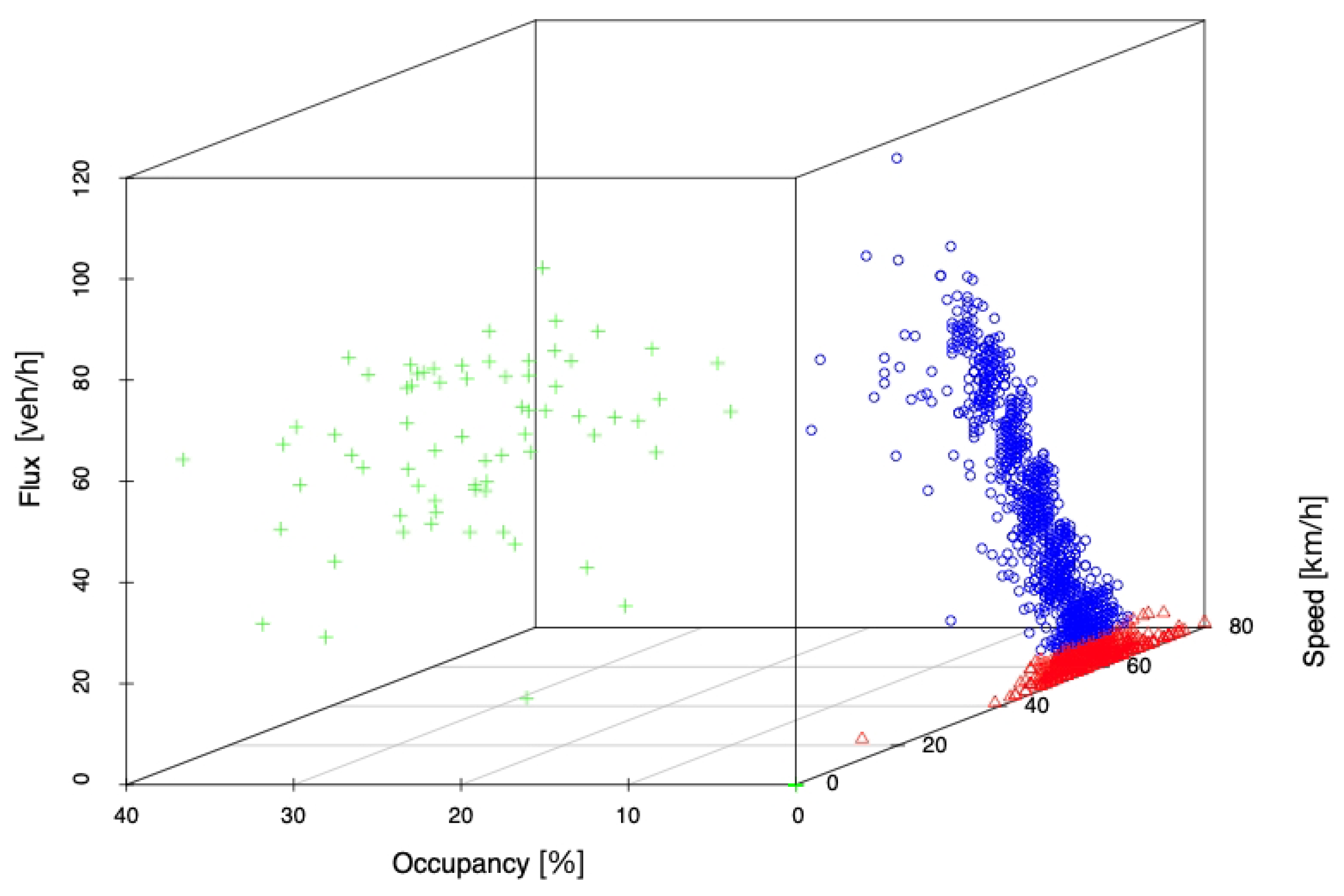
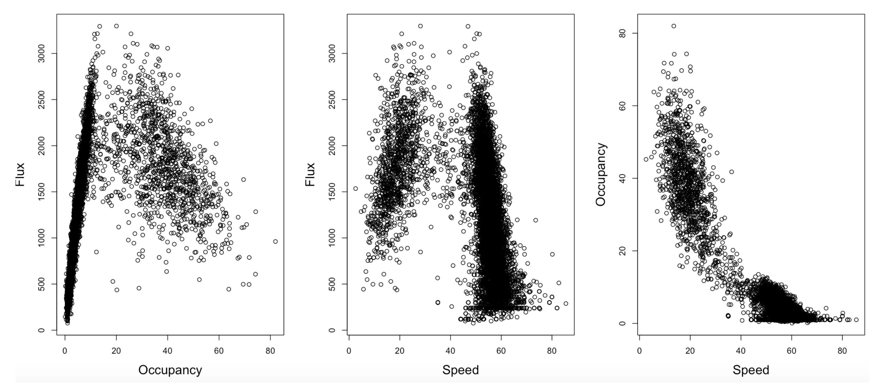
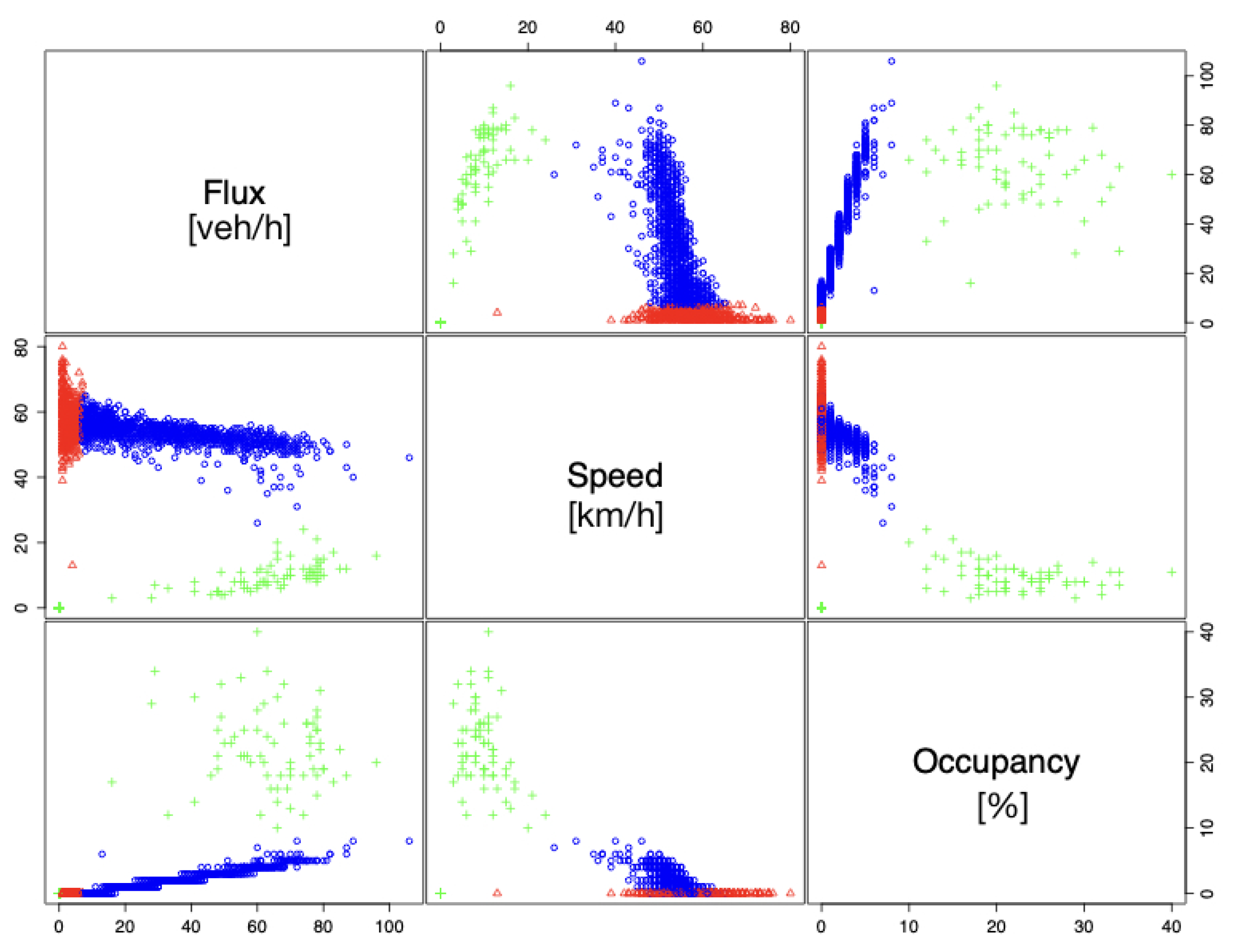
In this article, we focus on the FD for single roads by proposing a new approach to study the fundamental relationship among flow, density and speed. We propose novel statistical methodologies to analyze traffic data from fixed sensors, focusing on the three-leg relationships among the flow, density and speed. In particular, rather than considering the FD as a two-quantity relationship (flow–density or speed–density), we analyze data in the three-dimensional space represented by flow, density and speed. This allows us to better exploit the statistical tools, in particular for the analysis of traffic regimes.
We recall that, in equilibrium regimes, the fundamental relationship
dictates that traffic measurement points should lie on a three-dimensional surface (see, e.g., [
11] Figure 4.1). In reality, observed traffic largely deviates from equilibrium and usually exhibits
free and
congested phases, with the first corresponding to stable and regular traffic, while the second reflects delays and congestion. Moreover, in the early 2000s, Kerner [
12] introduced a tree-phase traffic theory, based on the distinction among
free flow,
synchronized flow and
wide-moving jam. The last two phases are associated with congested traffic.
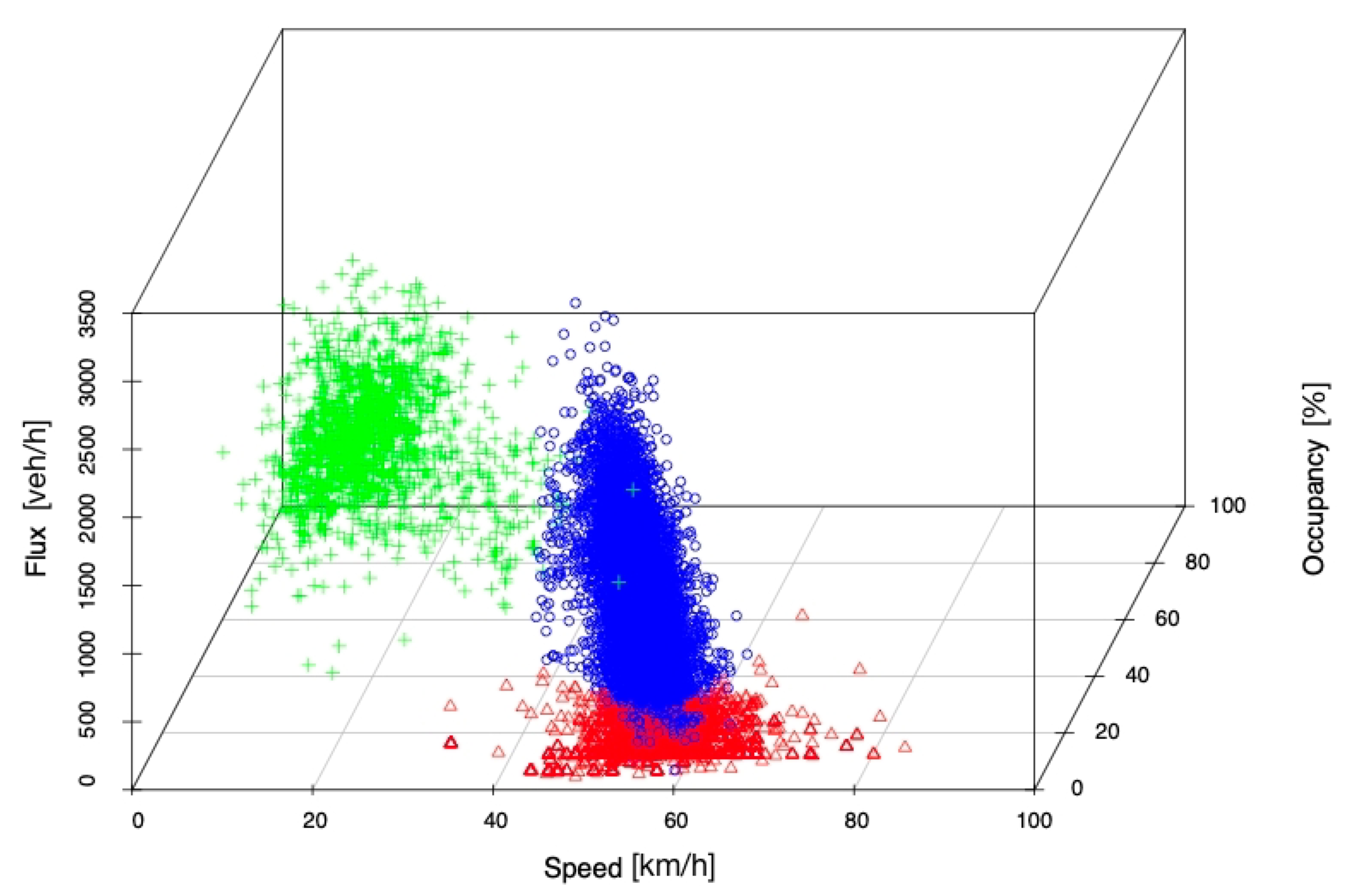
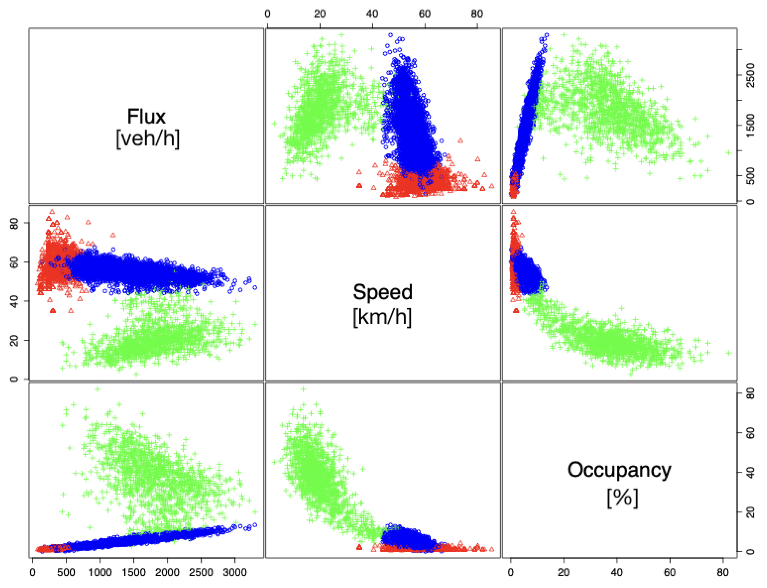
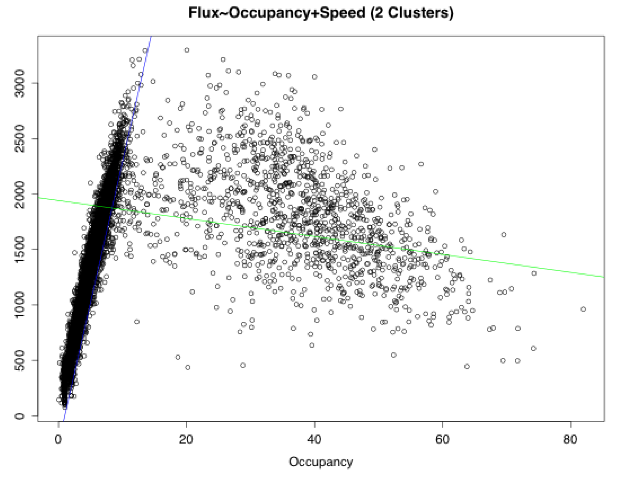
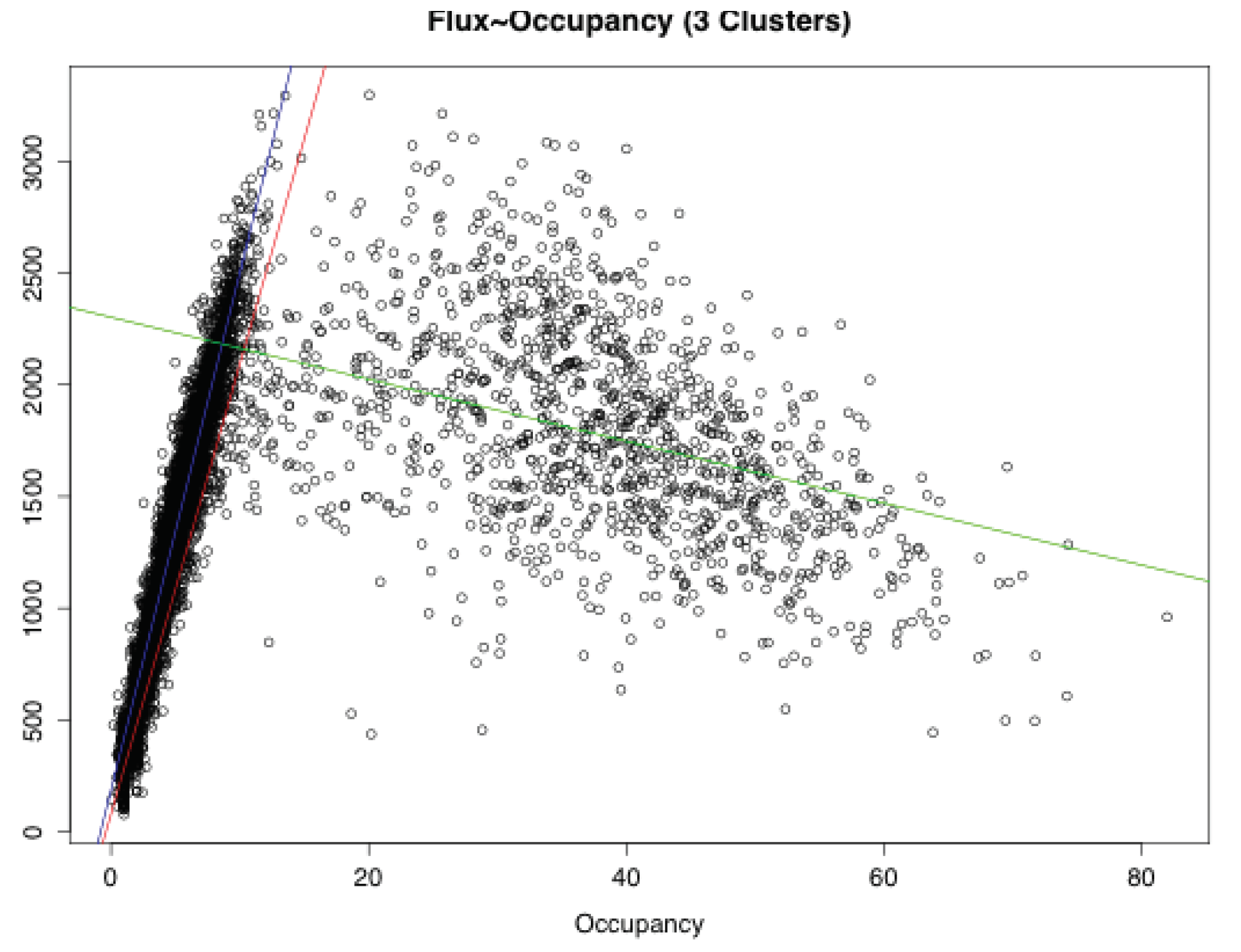
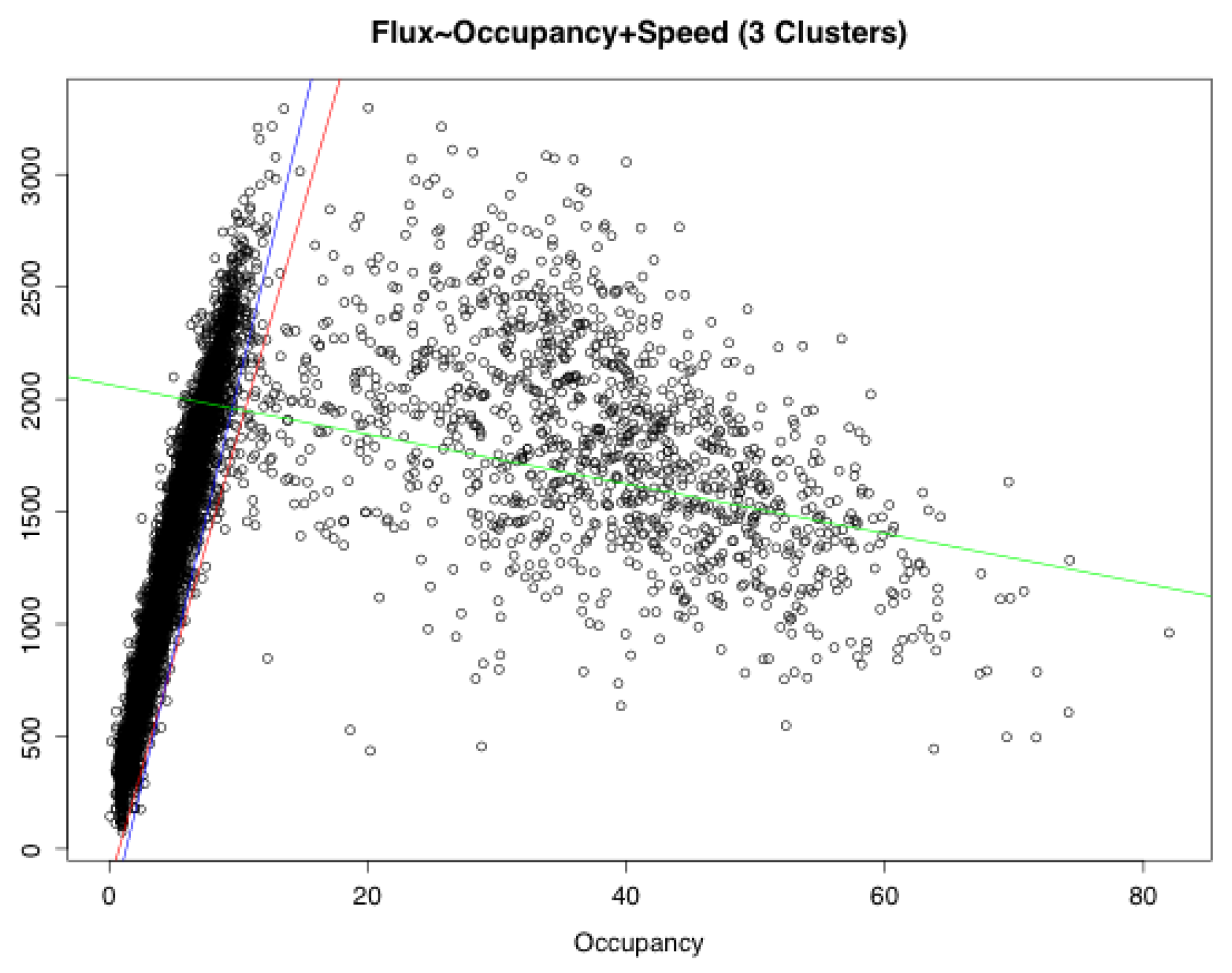
In this paper, using clustering methodologies, we are able to identify three traffic regimes, which are distinct in a statistically significant fashion. Interestingly, two regimes appear in what is commonly referred to as the free flow traffic and the third corresponds to the congested phase. This analysis does not contradict Kerner’s theory but rather points out that the static/stationary free-flow condition in the FD could exhibit two distinct phases, while the distinction of phases in congested traffic (e.g., Kerner’s model) is mainly dynamic.
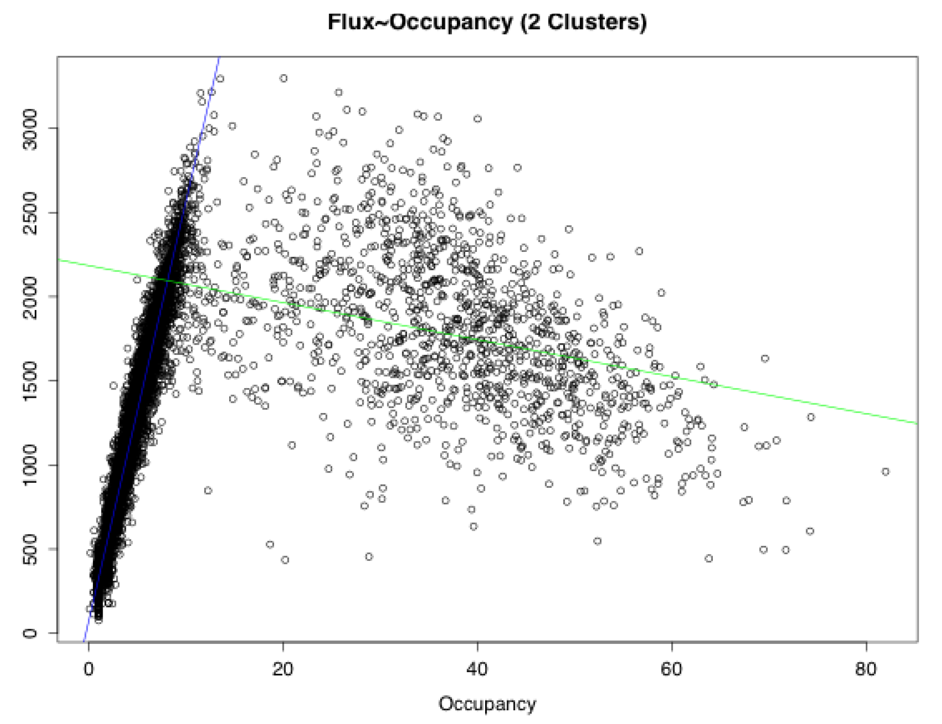
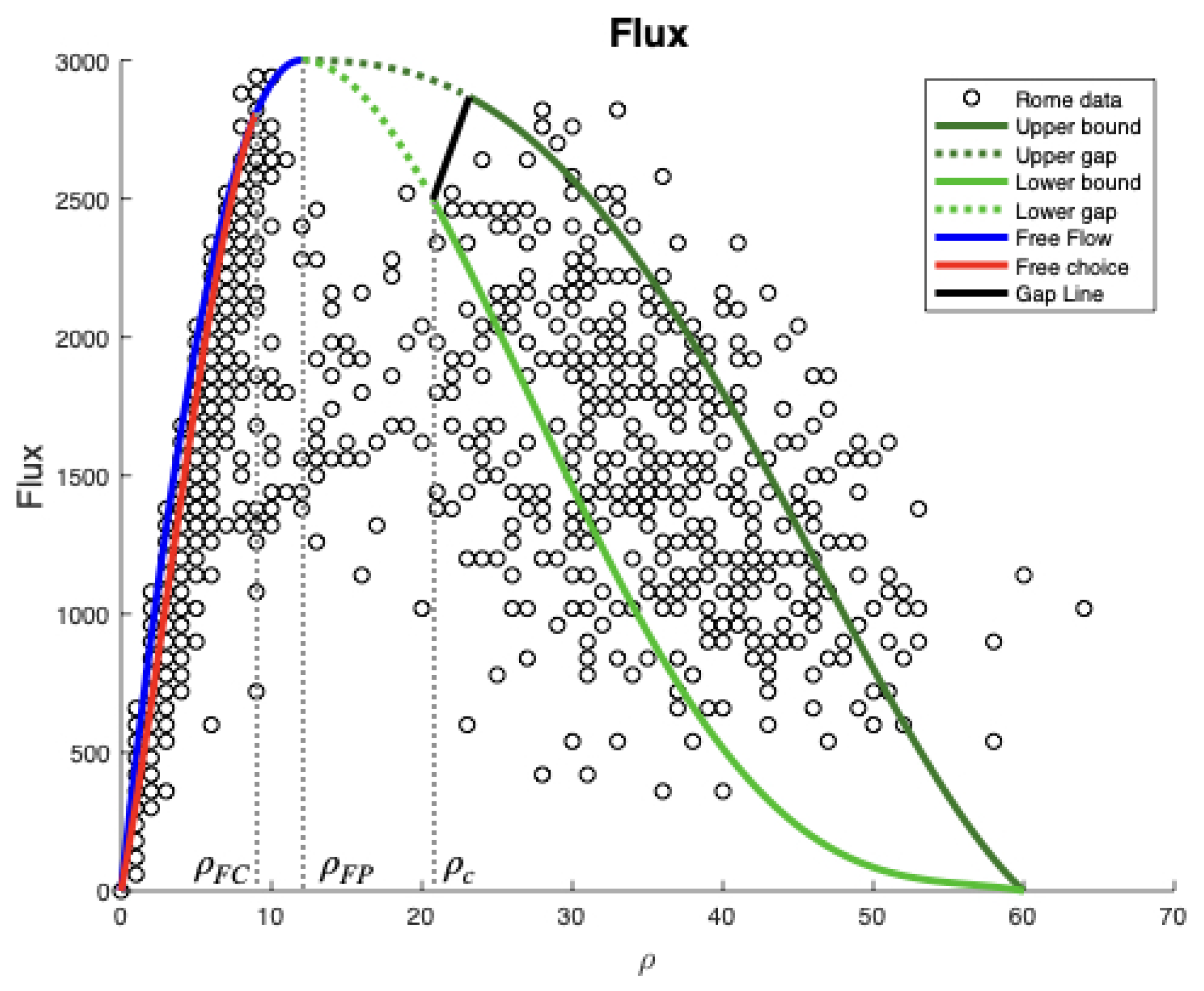
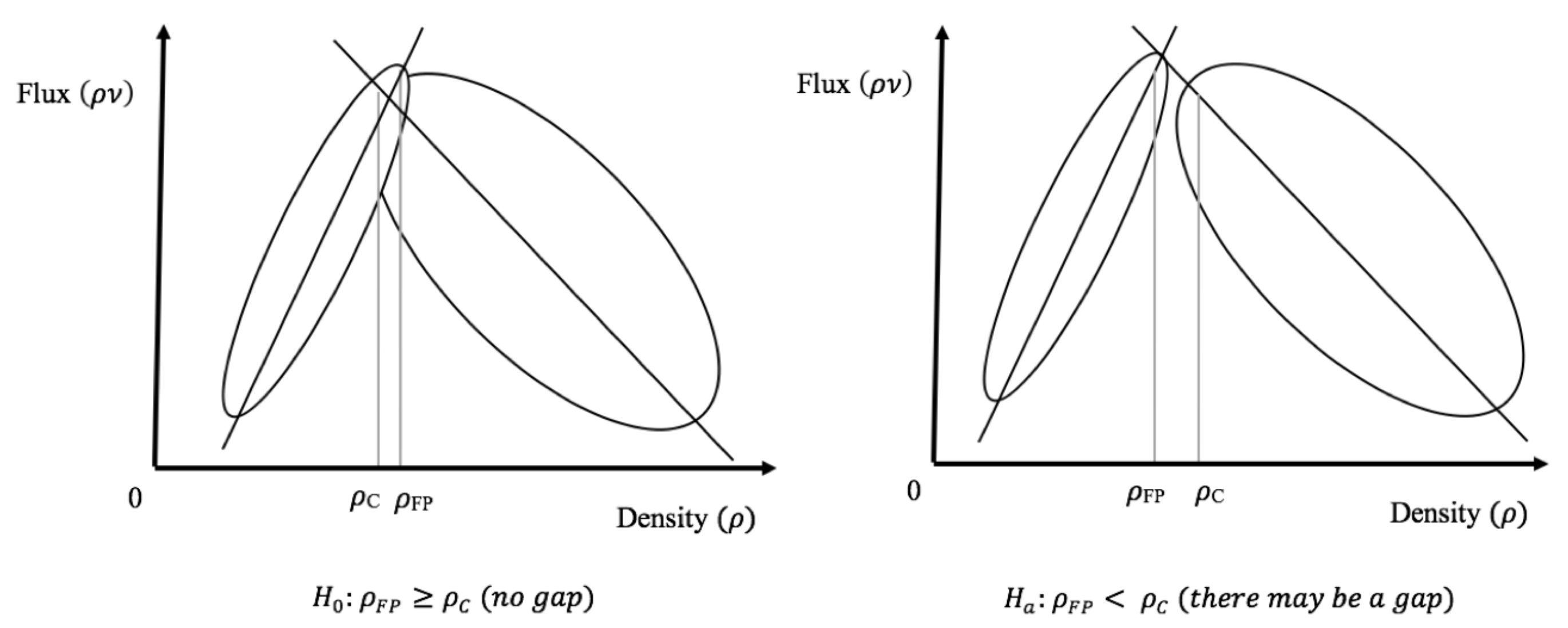
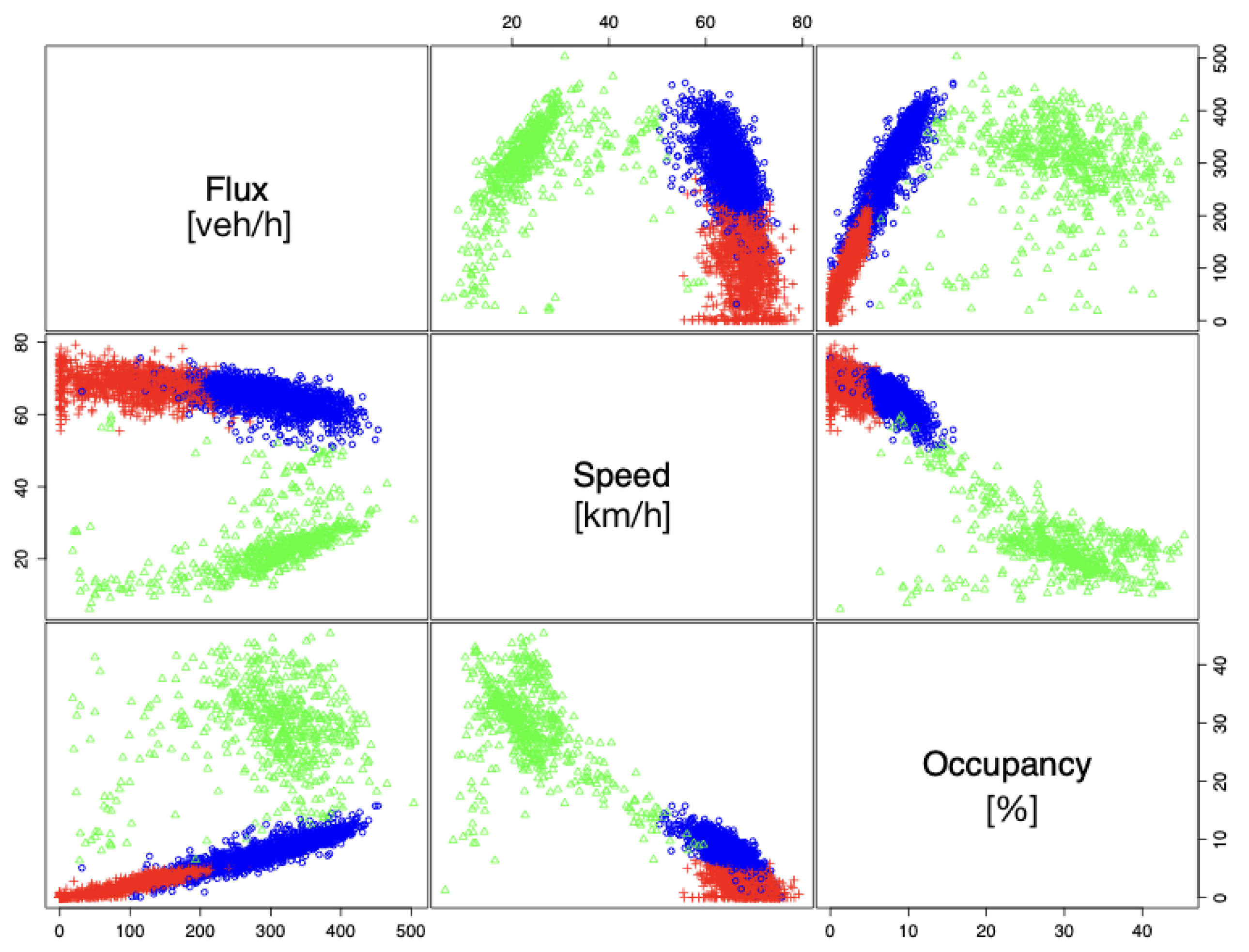
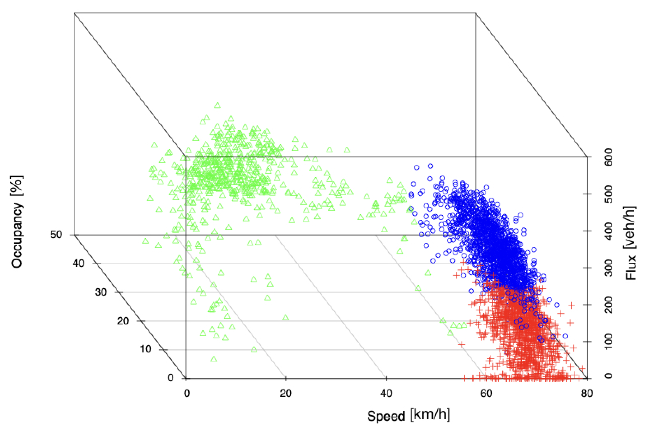
The second main empirical result of our paper is the clear evidence of the existence of a gap between the two phases of free flow and the congested one. While the appearance of such gap is best visualized in the 3D representation of the FD relationships, we use the classical flow–density relationship to statistically prove the existence of the gap. The main purpose is to prove the ubiquity (with respect to data collected at different geographical location and on different road types) of the gap in the classical setting and to enable a simpler analysis.
Building on the empirical evidence illustrated thus far, we propose a new three-phase macroscopic model. The LWR model is very popular in the traffic literature due to its simple mathematical representation. However, it has certain modeling limitations especially when it comes to describing complex wave structures such as stop and go waves, phantom jam and capacity drop. To overcome various limitations, Aw-Rascle [
3] and independently Zhang [
4] proposed a new model with conservation of a modified momentum. This so-called Aw-Rascle–Zhang (ARZ) model can be interpreted as part of a general family called General Second-Order Models (GSOM, see [
13]). Such models consist of the usual conservation of mass and the advective transport of a Lagrangian (or single driver) variable, which can represent, for instance, the desired speed of drivers. A recently proposed model of this category is the Collapsed Generalized ARZ model (CGARZ [
14]), where the driver speed depends on the Lagrangian variable only in the congested phase. Another line of research focuses on models showing two distinct phases, called the phase transition models [
6,
8,
9].
Our proposed model is a combination of the features offered by the ARZ, CGARZ and phase transition models. Our three-phase model not only has the characteristics of a CGARZ model with a gap among phases when analyzed in the flow–density space, but also exhibits the newly discovered phase when analyzed in the speed–density space. After showing how our model performs in data fitting, we provide a complete characterization of the characteristic curves and the solutions of the Riemann problems. The latter are the building block for solutions to Cauchy problems (see [
5]). To sum up, the main novelties and contributions of our paper are as follows:
Unlike most studies that focus on traffic data from a single source, we use data from multiple geographic locations in Europe and the US and analyze the fundamental relationships among flow, density and speed in the 3D space instead of the commonly adopted two-variable representation of the FD. In addition, we use a set of statistical tools including model-based clustering, hypothesis testing and regression to analyze the traffic data.
Following the above exercise, we discover three data clusters representing three traffic regimes, two of which are contained in the free-flow phase and the third corresponds to the congested phase. Moreover, we are able to detect a statistically significant gap between the first two regimes and the third one. These findings are validated using multiple data sources, and the main features (regimes and gaps) are consistent across different geographical areas.
Building on the first two, we propose a new three-phase macroscopic traffic flow model, which exhibits all the characteristics shown by our data analyses and combines the features of the ARZ, CGARZ and phase transition models. A complete characterization of solutions of the Riemann problems is provided.
The article is organized as follows. In
Section 2, we introduce the datasets, their statistical analysis and the results obtained. Moreover, we describe the impacts of these results on traffic modeling. Lastly, in
Section 3, we propose a new three-phase macroscopic model.
3. A Macroscopic Second-Order Model Accounting for the 3 Phases
Following the approach of Colombo et al. [
7], Fan et al. [
14], we propose a new macroscopic model accounting for the three phases derived in the previous sections. In conservation form, the model can be expressed as
where the velocity function is chosen such that
for some
, and it is continuous at
and
. In (
1)–(
2), the quantity
may represent various traffic characteristics, such as vehicles classes [
20], aggressiveness [
21], desired spacing [
22] or perturbation from equilibrium [
23], which are transported with the traffic stream. We refer to the variable
as a
total property [
14]. The function
v defined in (
2) must be:
Non-negative: for all , ;
Continuous: and for all
Vanishing at maximal density: for all
Non-decreasing with respect to w: for
With the above assumptions, the corresponding flux function satisfies for all w.
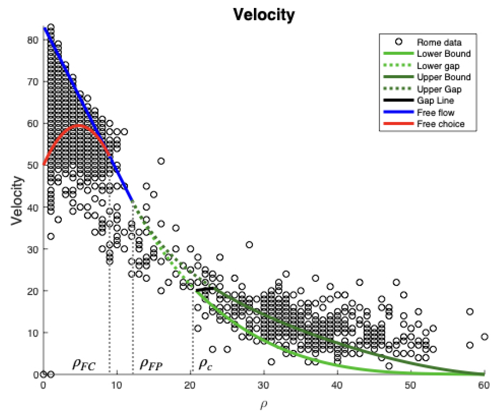
To take into account the possible presence of a gap, as suggested by our analysis, we fix the value
of the maximal speed in congestion, and let
be the density value such that
Defining the velocity function (see
Figure 3) as
the corresponding flux function
displays the desired gap between the free-flow and congested phases (see
Figure 4).
3.1. Riemann Solver
To simplify the construction, it is not restrictive to assume that the fundamental diagram is
-differentiable, i.e., we assume that
and
System (
1) is defined on the invariant domain
We note that, under the above assumptions on the velocity function
v,
if and only if
and
. The eigenvalues are given by
so the system is strictly hyperbolic for
as long as
. We note that the second characteristic field is linearly degenerate, giving origin to contact discontinuity waves, while the first characteristic field is genuinely non-linear if
holds. Moreover, the Riemann invariants of the systems are given by
w and
v. In particular, the iso-values
correspond to waves of the first family (we recall that the system belongs to Temple class, i.e., shock and rarefaction curves coincide) and the contact discontinuities verify
. More precisely, in the strictly concave case (
5) the elementary waves are constructed as follows.
1-rarefaction waves. Two points
and
are connected by a 1-rarefaction wave if and only if
1-shock waves. Two points
and
are connected by a 1-shock wave if and only if
In this case, the jump discontinuity moves with speed
2-contact discontinuity. Two points
and
are connected by a 2-contact wave if and only if
In the general (non-concave) case (see
Figure 4), the 1-waves consist of a concatenation of shocks and rarefactions (see ([
24]
Section 1)).
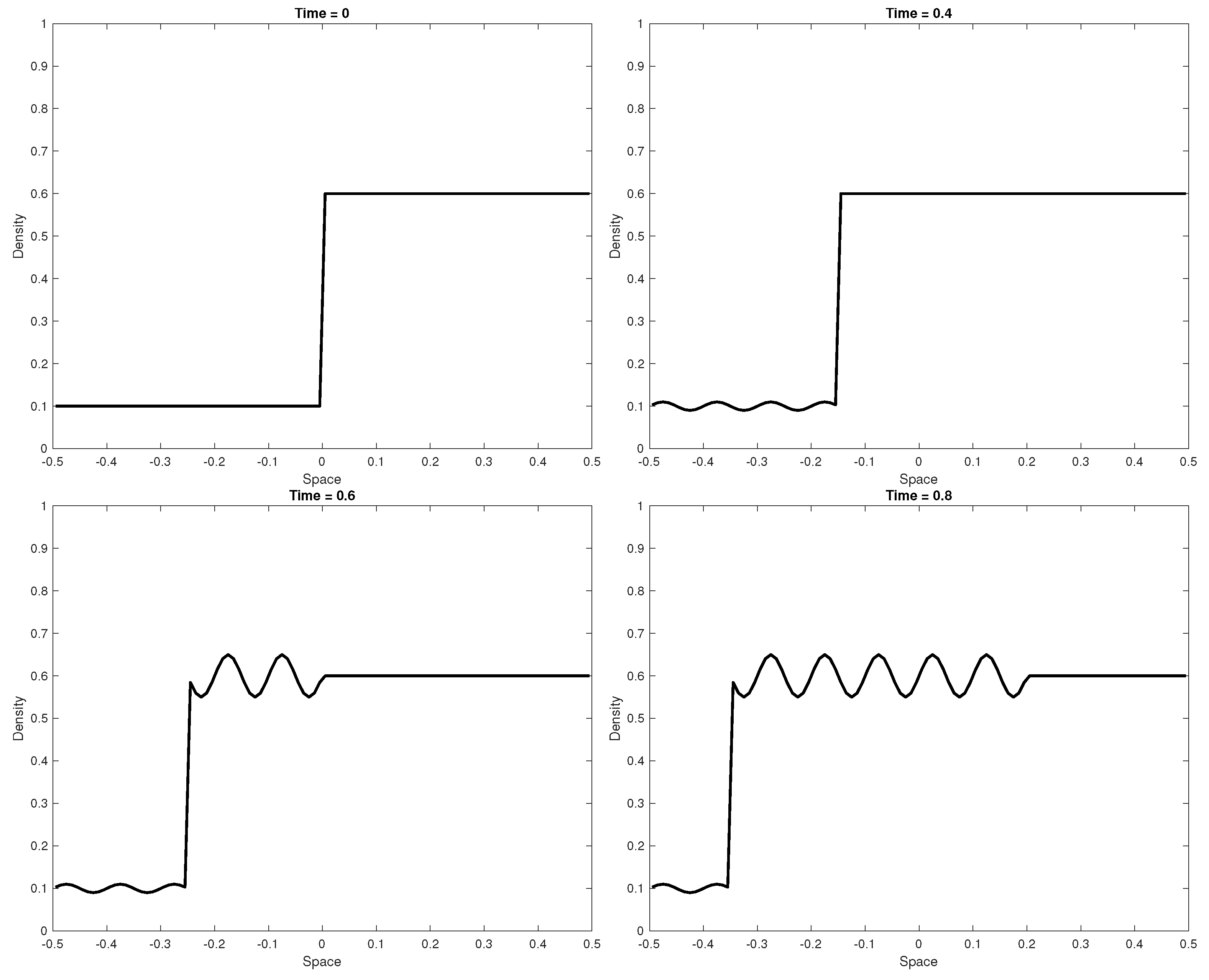
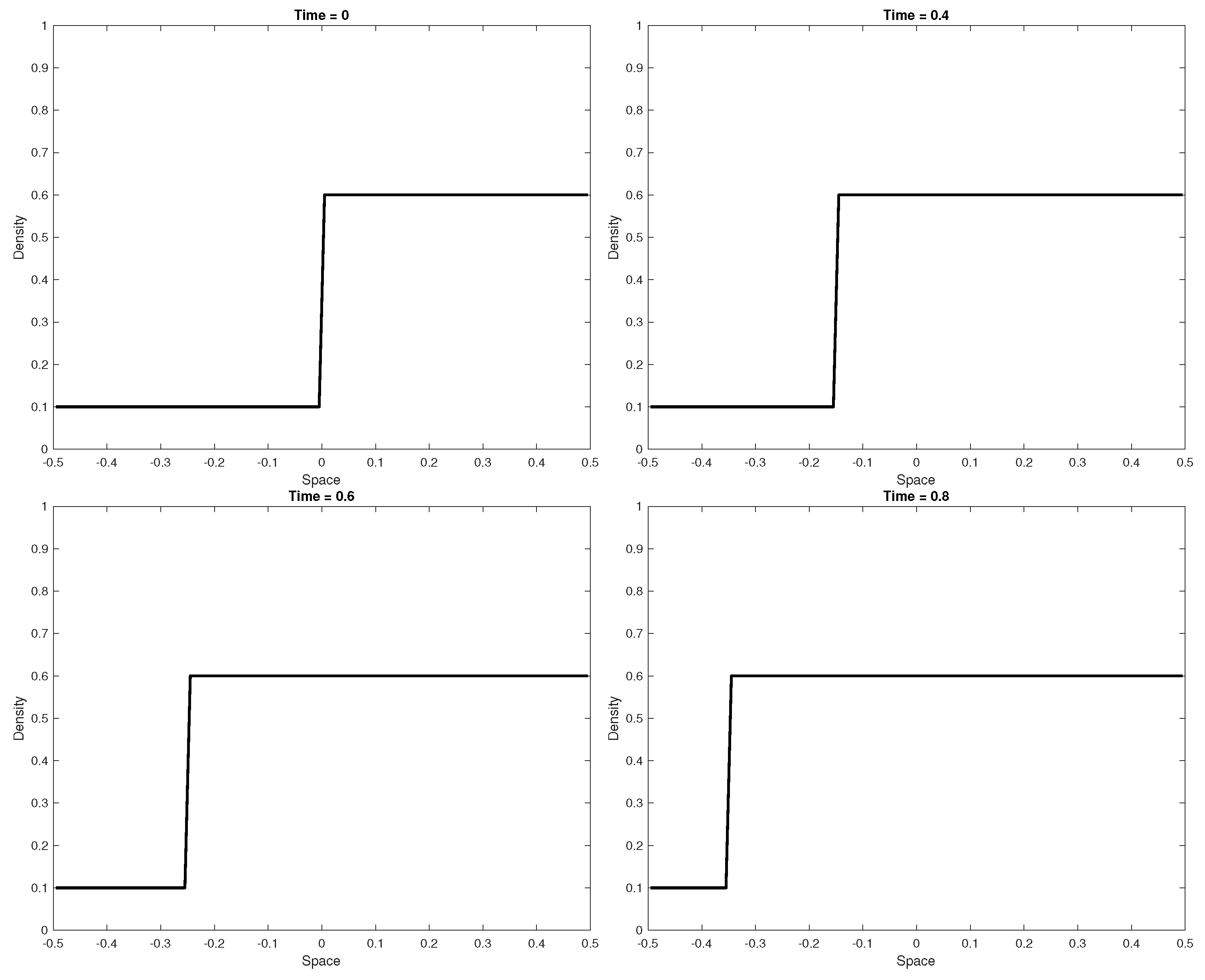
Based on the above elementary waves, the solution corresponding to general Riemann data
,
can be constructed as follows. Let
be the intermediate point defined by
Setting
,
is given by
In the latter case, a vacuum zone appears between the sector
The complete solution is then given by a 1-wave connecting and , followed by a 2-contact discontinuity between and (eventually separated by a vacuum zone if and ).
The presence of the gap between
and
does not modify the procedure, since the definition domain
is still invariant. We set
with
We can distinguish the following cases:
If and belongs both to or , the Riemann solver is defined as above.
If
and
, the intermediate point
belongs to
. Let
the point defined by
The solution is composed by 1-waves connecting
and
, a phase-transition jump between
and
moving with speed
followed by 1-waves connecting
and
and eventually a 2-contact from
to
.
If and , the intermediate point belongs to . Therefore, the solution always contains a 1-wave (shock phase-transition) from to , followed by a 2-contact discontinuity. Notice that the solution may also contain an intermediate 1-wave in the congested phase.


 ,
, 
