Relaxation Limit of the Aggregation Equation with Pointy Potential

Abstract

This work was devoted to the study of a relaxation limit of the so-called aggregation equation with a pointy potential in one-dimensional space. The aggregation equation is today widely used to model the dynamics of a density of individuals attracting each other through a potential. When this potential is pointy, solutions are known to blow up in final time. For this reason, measure-valued solutions have been defined. In this paper, we investigated an approximation of such measure-valued solutions thanks to a relaxation limit in the spirit of Jin and Xin. We study the convergence of this approximation and give a rigorous estimate of the speed of convergence in one dimension with the Newtonian potential. We also investigated the numerical discretization of this relaxation limit by uniformly accurate schemes.

1. Introduction

The so-called aggregation equation has been widely used to model the dynamics of a population of individuals in interaction. Let $W:\mathbb{R}\to \mathbb{R}$, sufficiently smooth, be the interaction potential governing the population. Then, in one dimension in space, the dynamics of the density of individuals, denoted by $\rho$, is governed by the following equation, for $t>0$ and $x\in \mathbb{R}$:

$${\partial }_t\rho +{\partial }_x\left(a\left[\rho \right]\rho \right)=0,\mathrm{with}a\left[\rho \right]=-W^{\prime }\ast \rho .$$

(1)

Such equations appear in many applications in population dynamics: for instance, to describe the collective migration of cells by swarming, the motion of bacteria by chemotaxis, the crowd motion, the flocking of birds, or fishes school, see, e.g., [1,2,3,4,5,6,7]. From a mathematical point of view, these equations have been widely studied. When the potential W is not smooth enough, it is known that weak solutions may blow up in finite time [8,9]. Thus, the existence of weak (measure) solutions has been investigated in, e.g., [10,11].

In this paper, we consider a relaxation limit in the spirit of Jin–Xin [12] of the aggregation equation in one space dimension on $\mathbb{R}$. It is now well-established that such modifications allow regularizing the solutions. For a given ${c>\parallel a\parallel }_{\infty }$, we introduce the system:

$$\begin{array}{cc}\hfill & {\partial }_t\rho +{\partial }_x\sigma =0,\hfill \end{array}$$

(2a)

$$\begin{array}{cc}\hfill & {\partial }_t\sigma +c^2{\partial }_x\rho =\frac{1}{\epsilon }(a\left[\rho \right]\rho -\sigma )\hfill \end{array}$$

(2b)

$$\begin{array}{cc}\hfill & a\left[\rho \right]=-W^{\prime }\ast \rho \hfill \end{array}$$

(2c)

This system is complemented by initial data ${\rho }_0$ and ${\sigma }_0:=a\left[{\rho }_0\right]{\rho }_0$. It is clear, at least formally, that when $\epsilon \to 0$, the solution $\rho$ of system (2) converges to the one of the aggregation Equations (1) (and it is actually only true if ${c>\parallel a\parallel }_{\infty }$). We mention that the aggregation equation may also be derived thanks to a hydrodynamical limit of kinetic equations [6,7,13].

The aim of this work was to study the convergence as $\epsilon \to 0$ of the relaxation system (2) towards the aggregation equation. More precisely, we establish a precise estimate of the speed of convergence, and we also illustrate with some numerical simulations. These estimates are obtained only in the case of the Newtonian potential in one dimension $W\left(x\right)=\frac{1}{2}\left|x\right|$. Indeed, in this particular case, we may link the aggregation equation to a scalar conservation law [14,15]. The same link holds for the relaxation system (2)—denoting:

$$u(t,x)=\frac{1}{2}-{\int }_{-\infty }^x\rho (t,dy),v(t,x)=\frac{1}{2}-{\int }_{-\infty }^x\sigma (t,dy),$$

where the notation $\int \rho (t,dy)$ stands for the integral with respect to the probability measure $\rho \left(t\right)$, then we verify easily that:

$$u=-W^{\prime }\ast \rho ,\rho =-{\partial }_{x}u,$$

so that $a\left[\rho \right]=u$. Then, integrating (2), we deduce that $(u,v)$ is a solution to:

$$\begin{array}{cc}\hfill & {\partial }_{t}u+{\partial }_{x}vs.=0\hfill \end{array}$$

(3a)

$$\begin{array}{cc}\hfill & {\partial }_{t}vs.+c^2{\partial }_{x}u=\frac{1}{\epsilon }\left(\frac{1}{2}{u}^2-v\right),\hfill \end{array}$$

(3b)

which is complemented with the initial data $u_0=\frac{1}{2}-{\int }_{-\infty }^x{\rho }_0\left(dy\right)$, and $v_0=\frac{1}{2}-{\int }_{-\infty }^x{\sigma }_0\left(dy\right)$. Clearly, as $\epsilon \to 0$, we expect that the solution of the above system converges to the solution of the following Burgers equation:

$${\partial }_{t}u+\frac{1}{2}{\partial }_x{u}^2=0.$$

Introducing the quantities $a=v-cu$ and $b=v+cu$, (3) is equivalent to the diagonalized system:

$$\begin{array}{cc}\hfill & {\partial }_{t}a-c{\partial }_{x}a=\frac{1}{\epsilon }\left(\frac{1}{2}{\left(\frac{b-a}{2c}\right)}^2-\frac{a+b}{2}\right)\hfill \end{array}$$

(4a)

$$\begin{array}{cc}\hfill & {\partial }_{t}b+c{\partial }_{x}b=\frac{1}{\epsilon }\left(\frac{1}{2}{\left(\frac{b-a}{2c}\right)}^2-\frac{a+b}{2}\right).\hfill \end{array}$$

(4b)

We will adapt the techniques developed in [16] to obtain convergence estimates for our system.

In order to illustrate this convergence result, numerical discretizations of the relaxation system (2) are investigated. The schemes we propose are such that they are uniform with respect to $\epsilon$, that is they satisfy the so-called asymptotic preserving (AP) property [17]. Therefore, such schemes in the limit $\epsilon \to 0$ must be consistent with the aggregation equation. The numerical simulations of solutions of the aggregation equation for pointy potentials have been studied by several authors, see, e.g., [11,13,18,19,20,21,22]. In particular, some authors pay attention to recover the correct behavior of the numerical solutions after the blow-up time. To do so, particular attention must be paid to the definition of the product $a\left[\rho \right]\rho$ when $\rho$ is a measure.

In this article, we propose two discretizations of the relaxation system which satisfy the AP property. In a first approach, we propose a simple splitting algorithm where we split the transport part and the right hand side in system (2). It results in a numerical scheme which is very simple to implement and for which we easily verify the AP property. The second approach relies on a well-balanced discretization in the spirit of [20,23]. This scheme is more expensive to implement than the first scheme, but its numerical solution has less diffusion, as it is illustrated by our numerical results.

The outline of the paper is the following. In Section 2, after recalling some useful notations, we prove our main result: an estimation of the speed of convergence in the Wasserstein $W_1$ distance with respect to $\epsilon$ of the solutions of the relaxation system (2) towards the solution of the aggregation Equation (1) in the case $W\left(x\right)=\frac{1}{2}\left|x\right|$. The numerical discretization is investigated in Section 3. Two numerical schemes verifying the AP property are proposed. The first scheme is based on a splitting algorithm, whereas the second scheme relies on a well-balanced discretization. Numerical results and comparisons are provided in Section 4.

2. Convergence Result

2.1. Notations

Before stating and proving our main results, we first recall some useful notations and results. Since we are dealing with conservation laws (in which the total mass is conserved), we will work in some space of probability measures, namely the Wasserstein space of order $p\ge 1$, which is the space of probability measures with a finite order p moment:

$${\mathcal{P}}_p\left({\mathbb{R}}^N\right)=\left\{\mu \mathrm{nonnegative}\mathrm{Borel}\mathrm{measure},\mu \left({\mathbb{R}}^N\right)=1,\int {\left|x\right|}^p\mu \left(dx\right)<\infty \right\}.$$

This space is endowed with the Wasserstein distance defined by (see, e.g., [24,25])

$$W_p(\mu ,\nu )=\underset{\gamma \in \Gamma (\mu ,\nu )}{inf}{\left\{{\int |y-x|}^p\gamma (dx,dy)\right\}}^{1/p},$$

(5)

where $\Gamma (\mu ,\nu )$ is the set of measures on ${\mathbb{R}}^N\times {\mathbb{R}}^N$ with marginals $\mu$ and $\nu$, meaning that:

$$\begin{array}{c}{\displaystyle \Gamma (\mu ,\nu )=\left\{\gamma \in {\mathcal{P}}_p({\mathbb{R}}^N\times {\mathbb{R}}^N);\forall \xi \in C_0\left({\mathbb{R}}^N\right),{\int }_{{\mathbb{R}}^{2N}}\xi \left(y_0\right)\gamma (d{y}_0,d{y}_1)={\int }_{{\mathbb{R}}^N}\xi \left(y_0\right)\mu \left(d{y}_0\right),\right.}\\ {\displaystyle \left.{\int }_{{\mathbb{R}}^{2N}}\xi \left(y_1\right)\gamma (d{y}_0,d{y}_1)={\int }_{{\mathbb{R}}^N}\xi \left(y_1\right)\nu \left(d{y}_1\right)\right\},}\end{array}$$

with $C_0\left({\mathbb{R}}^N\right)$, the set of continuous functions on ${\mathbb{R}}^N$ that vanish at infinity. From a simple minimization argument, we know that in the definition of $W_p$, the infimum is actually a minimum. A map that realizes the minimum in the definition (5) of $W_p$ is called an optimal transport plan, the set of which is denoted by ${\Gamma }_0(\mu ,\nu )$.

In the one-dimensional framework, we may simplify these definitions. Indeed, any probability measure $\mu$ on the real line $\mathbb{R}$ can be described in terms of its cumulative distribution function $F_{\mu }\left(x\right)=\mu \left((-\infty ,x)\right)$, which is a right-continuous and non-decreasing function with $F_{\mu }(-\infty )=0$ and $F_{\mu }(+\infty )=1$. Then, we can define the generalized inverse $F_{\mu }^{-1}$ of $F_{\mu }$ (or monotone rearrangement of $\mu$) by $F_{\mu }^{-1}\left(z\right):=inf\{x\in \mathbb{R}/F_{\mu }\left(x\right)>z\}$, it is a right-continuous and non-decreasing function as well, defined on $[0,1]$. We have for every non-negative Borel map $\xi$:

$${\int }_{\mathbb{R}}\xi \left(x\right)\mu \left(dx\right)={\int }_0^1\xi \left(F_{\mu }^{-1}\left(z\right)\right)dz.$$

In particular, $\mu \in {\mathcal{P}}_p\left(\mathbb{R}\right)$ if and only if $F_{\mu }^{-1}\in L^p(0,1)$. Moreover, in the one-dimensional setting, there exists a unique optimal transport plan realizing the minimum in (5). More precisely, if $\mu$ and $\nu$ belong to ${\mathcal{P}}_p\left(\mathbb{R}\right)$, with monotone rearrangements $F_{\mu }^{-1}$ and $F_{\nu }^{-1}$, then ${\Gamma }_0(\mu ,\nu )=\left\{{(F_{\mu }^{-1},F_{\nu }^{-1})}_{\#}{\mathbb{L}}_{(0,1)}\right\}$ where ${\mathbb{L}}_{(0,1)}$ is the restriction of the Lebesgue measure on $(0,1)$. Thus, we have the explicit expression of the Wasserstein distance (see [24,26,27]):

$$W_p(\mu ,\nu )={\left({\int }_0^1{|F_{\mu }^{-1}\left(z\right)-F_{\nu }^{-1}\left(z\right)|}^{p}dz\right)}^{1/p},$$

(6)

and the map $\mu \mapsto F_{\mu }^{-1}$ is an isometry between ${\mathcal{P}}_p\left(\mathbb{R}\right)$ and the convex subset of (essentially) non-decreasing functions of $L^p(0,1)$.

2.2. Convergence Estimates

Let us first consider the limit $\epsilon \to 0$ for the system (3). Compactness methods were used in [28] to get $L_{loc}^1$ convergence in space. However, in order to pass to the aggregation equation, one may want global $L^1$ convergence, which we prove in the following theorem, along the lines of Katsoulakis and Tzavaras [16].

Theorem 1.

Let$u_0\in L^{\infty }\cap BV\left(\mathbb{R}\right)$, $c>\parallel u_0{\parallel }_{L^{\infty }}$and set$v_0=\frac{u_0^2}{2}$. There exists a constant$C>0$such that, for any$\epsilon >0$, denoting by$(u^{\epsilon },v^{\epsilon })$the solution to (3) with initial data$(u_0,v_0)$, the following estimate holds:

$$\forall T>0,\parallel u\left(T\right)-u^{\epsilon }{\left(T\right)\parallel }_{L^1}\le CTV\left(u_0\right)(\sqrt{\epsilon T}+\epsilon ),$$

where u is the entropy solution to the Burgers equation with initial datum$u_0$.

Proof. 

Denote $(a^{\epsilon },b^{\epsilon })$ the solution to (4), and $G(a,b)=\frac{1}{2}{\left(\frac{b-a}{2c}\right)}^2-\frac{a+b}{2}$.

So as to obtain entropy inequalities on $(a^{\epsilon },b^{\epsilon })$, we need monotonicity properties on G. One can check that $G(a^{\epsilon },b^{\epsilon })$ is decreasing with respect to $a^{\epsilon }$ and $b^{\epsilon }$ if the so-called subcharacteristic condition $|u^{\epsilon }|<c$ holds. Up to a slight modification of the nonlinear term $f\left(u^{\epsilon }\right)=\frac{{\left(u^{\epsilon }\right)}^2}{2}$ in (3), which does not affect the value of $(a^{\epsilon },b^{\epsilon })$:

$$f\left(u\right):=\left\{\begin{array}{cc}-\parallel u_0\parallel u-{\displaystyle \frac{\parallel u_0{\parallel }^2}{2}},\hfill & \mathrm{if}u\le -\parallel u_0\parallel ,\hfill \\ {\displaystyle \frac{u^2}{2}},\hfill & \mathrm{if}-\parallel u_0\parallel \le u\le \parallel u_0\parallel ,\hfill \\ \parallel u_0\parallel u-{\displaystyle \frac{\parallel u_0{\parallel }^2}{2}},\hfill & \mathrm{if}\parallel u_0\parallel \le u,\hfill \end{array}\right.$$

the choice $c>\parallel u_0{\parallel }_{L^{\infty }}$ ensures that the subcharacteristic condition and the bound $\parallel u^{\epsilon }{\left(t\right)\parallel }_{L^{\infty }}\le {\parallel u_0\parallel }_{L^{\infty }}$ holds for all time.

Now, obtaining entropy inequalities on $(a^{\epsilon },b^{\epsilon })$ consists of making a comparison with constant state solutions to (4). Namely, letting $m=\parallel u_0{\parallel }_{L^{\infty }}\left(\frac{\parallel u_0{\parallel }_{L^{\infty }}}{2}-c\right)$, $M=\parallel u_0{\parallel }_{L^{\infty }}\left(\frac{\parallel u_0{\parallel }_{L^{\infty }}}{2}+c\right)$ and $h\left(a\right)=a+2c^2-2c\sqrt{c^2+2a}$, we have $G(k,h(k\left)\right)=0$ for all $k\in [m,M]$, and therefore $(k,h(k\left)\right)$ is a solution to (4). Thus, the following system holds:

$$\begin{array}{cc}\hfill & {\partial }_t(a^{\epsilon }-k)-c{\partial }_x(a^{\epsilon }-k)=\frac{1}{\epsilon }\left(G(a^{\epsilon },b^{\epsilon })-G(k,h\left(k\right))\right),\hfill \end{array}$$

(7a)

$$\begin{array}{cc}\hfill & {\partial }_t(b^{\epsilon }-h\left(k\right))+c{\partial }_x(b^{\epsilon }-h\left(k\right))=\frac{1}{\epsilon }\left(G(a^{\epsilon },b^{\epsilon })-G(k,h\left(k\right))\right).\hfill \end{array}$$

(7b)

Multiplying (7a) by $\mathrm{sgn}(a^{\epsilon }-k)$, (7b) by $\mathrm{sgn}(b^{\epsilon }-h\left(k\right))$ and summing yields:

$$\begin{array}{cc}\hfill & {\partial }_t\left(|a^{\epsilon }-k|+|b^{\epsilon }-h\left(k\right)|\right)-c{\partial }_x\left(|a^{\epsilon }-k|-|b^{\epsilon }-h\left(k\right)|\right)\hfill \\ \hfill & =\frac{1}{\epsilon }\left(\mathrm{sgn}(a^{\epsilon }-k)+\mathrm{sgn}(b^{\epsilon }-h\left(k\right))\right)\left(G(a^{\epsilon },b^{\epsilon })-G(k,h\left(k\right))\right).\hfill \end{array}$$

Hence, using the monotonicity of G, we obtain the following entropy inequalities on $(a^{\epsilon },b^{\epsilon })$:

$${\partial }_t\left(|a^{\epsilon }-k|+|b^{\epsilon }-h\left(k\right)|\right)-c{\partial }_x\left(|a^{\epsilon }-k|-|b^{\epsilon }-h\left(k\right)|\right)\le 0.$$

(8)

We now turn to proving the entropy inequalities on $u^{\epsilon }$. Straightforward computations yield the existence of a constant $C>0$ such that, for all $a,b\in [m,M]$, one has $\left|h\right(a)-b|\le C\left|G\right(a,b\left)\right|$. We therefore work on the variable $w^{\epsilon }:=\frac{h\left(a^{\epsilon }\right)-a^{\epsilon }}{2c}$ in the first place. Let $\kappa \in \left[-\parallel u_0{\parallel }_{L^{\infty }},{\parallel u_0\parallel }_{L^{\infty }}\right]$, and $k\in [m,M]$ such that $\kappa =\frac{h\left(k\right)-k}{2c}$. We have:

$$|w^{\epsilon }-\kappa |=\frac{1}{2c}\left(|h\left(a^{\epsilon }\right)-h\left(k\right)|+|a^{\epsilon }-k|\right)=\frac{1}{2c}\left(|a^{\epsilon }-k|+|b^{\epsilon }-h\left(k\right)|+r_1^{\epsilon }\right),$$

(9)

where $r_1^{\epsilon }=|h\left(a^{\epsilon }\right)-h\left(k\right)|-|b^{\epsilon }-h\left(k\right)|$ verifies $|r_1^{\epsilon }|\le |h\left(a^{\epsilon }\right)-b^{\epsilon }|\le C|G(a^{\epsilon },b^{\epsilon })|$. Thus, we are left to control $\left|G\right(a^{\epsilon },b^{\epsilon }\left)\right|$. To do so, we formally differentiate this quantity and use (4):

$$\begin{array}{cc}\hfill {\partial }_t\left|G(a^{\epsilon },b^{\epsilon })\right|& =\left({\partial }_t{a}^{\epsilon }{\partial }_{a}G(a^{\epsilon },b^{\epsilon })+{\partial }_t{b}^{\epsilon }{\partial }_{b}G(a^{\epsilon },b^{\epsilon })\right)\mathrm{sgn}\left(G(a^{\epsilon },b^{\epsilon })\right),\hfill \\ \hfill & =\frac{1}{\epsilon }\left({\partial }_{a}G(a^{\epsilon },b^{\epsilon })+{\partial }_{b}G(a^{\epsilon },b^{\epsilon })\right)\left|G(a^{\epsilon },b^{\epsilon })\right|\hfill \\ \hfill & -c\mathrm{sgn}\left(G(a^{\epsilon },b^{\epsilon })\right)\left({\partial }_x{a}^{\epsilon }{\partial }_{a}G(a^{\epsilon },b^{\epsilon })+{\partial }_x{b}^{\epsilon }{\partial }_{b}G(a^{\epsilon },b^{\epsilon })\right),\hfill \\ \hfill & \le \frac{1}{\epsilon }\underset{{[m,M]}^2}{sup}\left({\partial }_{a}G+{\partial }_{b}G\right)\left|G(a^{\epsilon },b^{\epsilon })\right|+c\underset{{[m,M]}^2}{sup}\left(|{\partial }_{a}G|+|{\partial }_{b}G|\right)\left(|{\partial }_x{a}^{\epsilon }|+|{\partial }_x{b}^{\epsilon }|\right).\hfill \end{array}$$

Integrating in space gives:

$$\frac{\mathrm{d}}{\mathrm{d}t}\parallel G(a^{\epsilon },b^{\epsilon }){\parallel }_{L^1}\le -\frac{A}{\epsilon }{\parallel G(a^{\epsilon },b^{\epsilon })\parallel }_{L^1}+B\left(TV\left(a_0\right)+TV\left(b_0\right)\right),$$

where $A=-{sup}_{{[m,M]}^2}({\partial }_{a}G+{\partial }_{b}G)$ and $B=c{sup}_{{[m,M]}^2}\left(\right|{\partial }_{a}G|+|{\partial }_{b}G\left|\right)$ are positive constants which do not depend on $\epsilon$ nor on time. A Gronwall lemma then gives:

$$\parallel G(a^{\epsilon }\left(t\right),b^{\epsilon }\left(t\right)){\parallel }_{L^1}\le C\left(TV\left(a_0\right)+TV\left(b_0\right)\right)\epsilon ,$$

(10)

where we still denote $C=B/A$ as a constant independent of time and of $\epsilon$.

In addition, since, $G(a,h(a\left)\right)=0$, one has $\frac{1}{2}{\left(\frac{h\left(a\right)-a}{2c}\right)}^2=\frac{1}{2}(h\left(a\right)+a)$ and therefore:

$$\begin{array}{cc}\hfill \mathrm{sgn}(w^{\epsilon }-\kappa )\left(\frac{{\left(w^{\epsilon }\right)}^2}{2}-\frac{{\kappa }^2}{2}\right)& =\frac{1}{2}\mathrm{sgn}\left(h\left(a^{\epsilon }\right)-h\left(k\right)-(a^{\epsilon }-k)\right)\left(h\left(a^{\epsilon }\right)+a^{\epsilon }-(h\left(k\right)+k)\right),\hfill \\ \hfill & =\frac{1}{2}\left(|h\left(a^{\epsilon }\right)-h\left(k\right)|-|a^{\epsilon }-k|\right),\hfill \\ \hfill & =\frac{1}{2}\left(|b-h\left(k\right)|-|a^{\epsilon }-k|+r_2^{\epsilon }\right),\hfill \end{array}$$

(11)

with $|r_2^{\epsilon }|\le C|G(a^{\epsilon },b^{\epsilon })|$. Differentiating (9) in time and (11) in space, and using (8) thus yields:

$${\partial }_t|w^{\epsilon }-\kappa |+{\partial }_x\mathrm{sgn}(w^{\epsilon }-\kappa )\left(\frac{{\left(w^{\epsilon }\right)}^2}{2}-\frac{{\kappa }^2}{2}\right)\le \frac{1}{2c}\left({\partial }_t{r}_1^{\epsilon }+c{\partial }_x{r}_2^{\epsilon }\right).$$

(12)

Then, we estimate $\parallel u\left(t\right)-w^{\epsilon }{\left(t\right)\parallel }_{L^1}$ using Kuznetsov’s doubling of variables technique (see, e.g., [29] for scalar conservation laws with viscosity and [30] for a more general formalism) in order to combine (12) with Kruzkov inequalities on the entropy solution u, that read:

$${\partial }_t|u-\kappa |+{\partial }_x\mathrm{sgn}(u-\kappa )\left(f\left(u\right)-f\left(\kappa \right)\right)\le 0.$$

(13)

Writing, respectively, (13) at point $(s,x)$ for $\kappa =w^{\epsilon }(t,y)$ and (12) at point $(t,y)$ for $\kappa =u(s,x)$, we obtain:

$$\begin{array}{cc}\hfill & {\partial }_s|u(s,x)-w^{\epsilon }(t,y)|+{\partial }_x\mathrm{sgn}(u(s,x)-w^{\epsilon }(t,y))\left(\frac{u{(s,x)}^2}{2}-\frac{{\left(w^{\epsilon }(t,y)\right)}^2}{2}\right)\le 0,\hfill \end{array}$$

(14a)

$$\begin{array}{cc}\hfill & {\partial }_t|w^{\epsilon }(t,y)-u(s,x)|+{\partial }_y\mathrm{sgn}(w^{\epsilon }(t,y)-u(s,x))\left(\frac{{\left(w^{\epsilon }(t,y)\right)}^2}{2}-\frac{u{(s,x)}^2}{2}\right)\hfill \\ \hfill & \le \frac{1}{2c}\left({\partial }_t{r}_1^{\epsilon }(t,y)+c{\partial }_y{r}_2^{\epsilon }(t,y)\right).\hfill \end{array}$$

(14b)

Now, let ${\omega }_{\alpha }\left(t\right)=\frac{1}{\alpha }\omega \left(\frac{t}{\alpha }\right)$ and ${\Omega }_{\beta }\left(x\right)=\frac{1}{\beta }\Omega \left(\frac{x}{\beta }\right)$ be two mollyfing kernels. Setting $g(s,t,x,y)={\omega }_{\alpha }(s-t){\Omega }_{\beta }(x-y)$ and testing (14a) and (14b) against $g(·,t,·,y){𝟙}_{[0,T]}$ and $g(s,·,x,·){𝟙}_{[0,T]}$, respectively, and integrating over $[0,T]\times \mathbb{R}$, we obtain on the one hand:

$$\begin{array}{cc}\hfill & \int \int \int \int {\partial }_{s}g(s,t,x,y)|u(s,x)-w^{\epsilon }(t,y)|\mathrm{d}s\mathrm{d}x\mathrm{d}t\mathrm{d}y\hfill \\ \hfill & +\int \int \int \int {\partial }_{x}g(s,t,x,y)\mathrm{sgn}(u(s,x)-w^{\epsilon }(t,y))\left(\frac{u{(s,x)}^2}{2}-\frac{{\left(w^{\epsilon }(t,y)\right)}^2}{2}\right)\mathrm{d}s\mathrm{d}x\mathrm{d}t\mathrm{d}y\hfill \\ \hfill & -\int \int \int g(T,t,x,y)|u(T,x)-w^{\epsilon }(t,y)|\mathrm{d}x\mathrm{d}t\mathrm{d}y\hfill \\ \hfill & +\int \int \int g(0,t,x,y)|u(0,x)-w^{\epsilon }(t,y)|\mathrm{d}x\mathrm{d}t\mathrm{d}y\ge 0,\hfill \end{array}$$

(15)

and on the other hand:

$$\begin{array}{cc}\hfill & \int \int \int \int {\partial }_{t}g(s,t,x,y)|w^{\epsilon }(t,y)-u(s,x)|\mathrm{d}s\mathrm{d}x\mathrm{d}t\mathrm{d}y\hfill \\ \hfill & +\int \int \int \int {\partial }_{y}g(s,t,x,y)\mathrm{sgn}(w^{\epsilon }(t,y)-u(s,x))\left(\frac{{\left(w^{\epsilon }(t,y)\right)}^2}{2}-\frac{u{(s,x)}^2}{2}\right)\mathrm{d}s\mathrm{d}x\mathrm{d}t\mathrm{d}y\hfill \\ \hfill & -\int \int \int g(s,T,x,y)|w^{\epsilon }(T,y)-u(s,x)|\mathrm{d}s\mathrm{d}x\mathrm{d}y+\int \int \int g(s,0,x,y)|w^{\epsilon }(0,y)-u(s,x)|\mathrm{d}s\mathrm{d}x\mathrm{d}y\hfill \\ \hfill & \ge \frac{1}{2c}(\int \int \int \int {\partial }_{t}g(s,t,x,y)r_1^{\epsilon }(t,y)\mathrm{d}s\mathrm{d}x\mathrm{d}t\mathrm{d}y+c\int \int \int \int {\partial }_{y}g(s,t,x,y)r_2^{\epsilon }(t,y)\mathrm{d}s\mathrm{d}x\mathrm{d}t\mathrm{d}y\hfill \\ \hfill & -\int \int \int g(s,T,x,y)r_1^{\epsilon }(T,y)\mathrm{d}s\mathrm{d}x\mathrm{d}y+\int \int \int g(s,0,x,y)r_1^{\epsilon }(0,y)\mathrm{d}s\mathrm{d}x\mathrm{d}y)=:\mathrm{RHS}.\hfill \end{array}$$

(16)

Now, since $|·|$ is even, and ${\partial }_{s}g=-{\partial }_{t}g$ and ${\partial }_{x}g=-{\partial }_{y}g$, we deduce by adding (15) and (16):

$$\begin{array}{cc}\hfill & -\int \int \int g(T,t,x,y)|u(T,x)-w^{\epsilon }(t,y)|\mathrm{d}x\mathrm{d}t\mathrm{d}y\hfill \\ \hfill & +\int \int \int g(0,t,x,y)|u(0,x)-w^{\epsilon }(t,y)|\mathrm{d}x\mathrm{d}t\mathrm{d}y\hfill \\ \hfill & -\int \int \int g(s,T,x,y)|u(s,x)-w^{\epsilon }(T,y)|\mathrm{d}s\mathrm{d}x\mathrm{d}y\hfill \\ \hfill & +\int \int \int g(s,0,x,y)|u(s,x)-w^{\epsilon }(0,y)|\mathrm{d}s\mathrm{d}x\mathrm{d}y\ge \mathrm{RHS}.\hfill \end{array}$$

(17)

Then, we write:

$$\begin{array}{cc}\hfill \parallel u\left(T\right)-w^{\epsilon }{\left(T\right)\parallel }_{L^1}& =\int \int \int {\omega }_{\alpha }(T-t){\Omega }_{\beta }(x-y)|u(T,y)-w^{\epsilon }(T,y)|\mathrm{d}x\mathrm{d}t\mathrm{d}y\hfill \\ \hfill & +\int \int \int {\omega }_{\alpha }(s-T){\Omega }_{\beta }(x-y)|u(T,y)-w^{\epsilon }(T,y)|\mathrm{d}s\mathrm{d}x\mathrm{d}y,\hfill \\ \hfill & =:I_1+I_2.\hfill \end{array}$$

(18)

A triangle inequality gives for $I_1$:

$$\begin{array}{cc}\hfill I_1& \le \int \int \int {\omega }_{\alpha }(T-t){\Omega }_{\beta }(x-y)|u(T,y)-u(T,x)|\mathrm{d}x\mathrm{d}t\mathrm{d}y\hfill \\ \hfill & +\int \int \int {\omega }_{\alpha }(T-t){\Omega }_{\beta }(x-y)|u(T,x)-w^{\epsilon }(t,y)|\mathrm{d}x\mathrm{d}t\mathrm{d}y\hfill \\ \hfill & +\int \int \int {\omega }_{\alpha }(T-t){\Omega }_{\beta }(x-y)|w^{\epsilon }(t,y)-w^{\epsilon }(T,y)|\mathrm{d}x\mathrm{d}t\mathrm{d}y\hfill \\ \hfill & =:T_1+T_2+T_3.\hfill \end{array}$$

with $T_1\le C\beta ·TV\left(u_0\right)$, the second term $T_2$ appearing in (17) and for the last one we write:

$$T_3\le {\int }_{\mathbb{R}}{\Omega }_{\beta }(x-y){\int }_0^T{\omega }_{\alpha }(T-t){\int }_{\mathbb{R}}|w^{\epsilon }(t,y)-w^{\epsilon }(T,y)|\mathrm{d}y\mathrm{d}t\mathrm{d}x,$$

and then we use the fact that $w^{\epsilon }$ is uniformely Lipschitz in $L^1\left(\mathbb{R}\right)$ with respect to $\epsilon$. Indeed, one has ${\partial }_t{w}^{\epsilon }=\frac{{\partial }_t{a}^{\epsilon }(h^{\prime }\left(a^{\epsilon }\right)-1)}{2c}$ with $h^{\prime }\left(a^{\epsilon }\right)-1$ being uniformely bounded with respect to $\epsilon$ as $a^{\epsilon }$ stays in the compact set $[m,M]$ for all time. In addition, estimating $\parallel {\partial }_t{a}^{\epsilon }{\left(t\right)\parallel }_{L^1}$ can be done reusing (4) and (10):

$$\parallel {\partial }_t{a}^{\epsilon }{\left(t\right)\parallel }_{L^1}\le c\parallel {\partial }_x{a}^{\epsilon }{\left(t\right)\parallel }_{L^1}+\frac{1}{\epsilon }{\parallel G(a^{\epsilon }\left(t\right),b^{\epsilon }\left(t\right))\parallel }_{L^1}\le C\left(TV\left(a_0\right)+TV\left(b_0\right)\right).$$

with $C>0$ still independent of time and of $\epsilon$. Hence, $\parallel {\partial }_t{w}^{\epsilon }{\left(t\right)\parallel }_{L^1}\le C\left(TV\left(a_0\right)+TV\left(b_0\right)\right)$ and $T_3\le \alpha C\left(TV\left(a_0\right)+TV\left(b_0\right)\right)$. All in all, we get for $I_1$:

$$\begin{array}{cc}\hfill I_1\le & \int \int \int {\omega }_{\alpha }(T-t){\Omega }_{\beta }(x-y)|u(T,x)-w^{\epsilon }(t,y)|\mathrm{d}x\mathrm{d}t\mathrm{d}y+C\beta ·TV\left(u_0\right)\hfill \\ \hfill & +\alpha C\left(TV\left(a_0\right)+TV\left(b_0\right)\right).\hfill \end{array}$$

Moreover, similarly, for $I_2$:

$$I_2\le \int \int \int {\omega }_{\alpha }(s-T){\Omega }_{\beta }(x-y)|u(s,x)-w^{\epsilon }(T,y)|\mathrm{d}s\mathrm{d}x\mathrm{d}y+C(\alpha +\beta )TV\left(u_0\right).$$

Returning to (18), we obtain:

$$\begin{array}{cc}\hfill \parallel u\left(T\right)-w^{\epsilon }{\left(T\right)\parallel }_{L^1}& \le \int \int \int {\omega }_{\alpha }\left(t\right){\Omega }_{\beta }(x-y)|u(0,x)-w^{\epsilon }(t,y)|\mathrm{d}x\mathrm{d}t\mathrm{d}y\hfill \end{array}$$

(19)

$$\begin{array}{cc}\hfill & +\int \int \int {\omega }_{\alpha }\left(s\right){\Omega }_{\beta }(x-y)|u(s,x)-w^{\epsilon }(0,y)|\mathrm{d}s\mathrm{d}x\mathrm{d}y-RHS\hfill \end{array}$$

(20)

$$\begin{array}{cc}\hfill & +\alpha C\left(TV\left(a_0\right)+TV\left(b_0\right)\right)+C(\alpha +\beta )TV\left(u_0\right).\hfill \end{array}$$

(21)

However, using a triangle inequality, one can show that:

$$\int \int \int {\omega }_{\alpha }\left(t\right){\Omega }_{\beta }(x-y)|u_0\left(x\right)-w^{\epsilon }(t,y)|\mathrm{d}x\mathrm{d}t\mathrm{d}y\le C\beta ·TV\left(u_0\right)+\alpha C\left(TV\left(a_0\right)+TV\left(b_0\right)\right),$$

and similarly:

$$\int \int \int {\omega }_{\alpha }\left(s\right){\Omega }_{\beta }(x-y)|u(s,x)-w^{\epsilon }(0,y)|\mathrm{d}s\mathrm{d}x\mathrm{d}y\le C(\alpha +\beta )TV\left(u_0\right).$$

We then bound from above the term RHS using inequality $\parallel r_i^{\epsilon }{\left(t\right)\parallel }_{L^1}\le C\left(TV\left(a_0\right)+TV\left(b_0\right)\right)\epsilon$ for $i=1,2$:

$$\begin{array}{cc}\hfill \left|\mathrm{RHS}\right|& =\frac{1}{2c}|\frac{1}{\alpha }\int \int \int \int {\omega }^{\prime }\left(\frac{s-t}{\alpha }\right){\Omega }_{\beta }(x-y)r_1^{\epsilon }(t,y)\mathrm{d}s\mathrm{d}x\mathrm{d}t\mathrm{d}y\hfill \\ \hfill & +\frac{c}{\beta }\int \int \int \int {\omega }_{\alpha }(s-t){\Omega }^{\prime }(x-y)r_2^{\epsilon }(t,y)\mathrm{d}s\mathrm{d}x\mathrm{d}t\mathrm{d}y\hfill \\ \hfill & -\int \int \int {\omega }_{\alpha }(s-T){\Omega }_{\beta }(x-y)r_1^{\epsilon }(T,y)\mathrm{d}s\mathrm{d}x\mathrm{d}y\hfill \\ \hfill & +\int \int \int {\omega }_{\alpha }\left(s\right){\Omega }_{\beta }(x-y)r_1^{\epsilon }(0,y)\mathrm{d}s\mathrm{d}x\mathrm{d}y|,\hfill \\ \hfill & \le C\left(\frac{T}{\alpha }+\frac{T}{\beta }+1\right)·\left(TV\left(a_0\right)+TV\left(b_0\right)\right)\epsilon .\hfill \end{array}$$

Finally, we obtain:

$$\begin{array}{cc}\hfill \parallel u\left(T\right)-w^{\epsilon }{\left(T\right)\parallel }_{L^1}\le & C\left(\frac{T}{\alpha }+\frac{T}{\beta }+1\right)\left(TV\left(a_0\right)+TV\left(b_0\right)\right)\epsilon \hfill \\ \hfill & +C(\alpha +\beta )TV\left(u_0\right)+\alpha C\left(TV\left(a_0\right)+TV\left(b_0\right)\right),\hfill \end{array}$$

which, after optimizing the values of $\alpha$ and $\beta$ and noticing that $TV\left(a_0\right),TV\left(b_0\right)\le C·TV\left(u_0\right)$, gives:

$$\parallel u\left(T\right)-w^{\epsilon }{\left(T\right)\parallel }_{L^1}\le CTV\left(u_0\right)(\sqrt{\epsilon T}+\epsilon ),$$

and this inequality, along with $\left|h\right(a)-b|\le C\left|G\right(a,b\left)\right|$ and (10) gives in turn the result. □

Denoting $\rho =-{\partial }_{x}u$, the convergence of $u^{\epsilon }\left(t\right)$ towards $u\left(t\right)$ in $L^1\left(\mathbb{R}\right)$ ensures that $\rho \left(t\right)$ is a probability measure. Indeed, since for all $\epsilon >0$, ${\rho }^{\epsilon }=-{\partial }_x{u}^{\epsilon }$ is a non-negative distribution, so is $\rho$. The Riesz–Markov theorem then ensures that $\rho$ can be represented by a non-negative Borel measure. In addition, almost everywhere, for $t\ge 0$, $u^{\epsilon }\left(t\right)$ is a non-increasing function taking values in $[0,1]$ and hence converges to a certain limit when x goes to $+\infty$. The same holds true for the limit function $u\left(t\right)$. However, since $u^{\epsilon }\left(t\right)-u\left(t\right)\in L^1\left(\mathbb{R}\right)$, then $u^{\epsilon }(t,x)-u(t,x)$ must vanish as x goes to $+\infty$. Therefore, the total mass of $\rho \left(t\right)$ is 1.

Then, passing to the relaxation system (2) for the aggregation Equation (1) can be done by using (6) with $p=1$. As a consequence, Theorem 1 translates as follows for the aggregation.

Theorem 2.

Let${\rho }_0\in {\mathcal{P}}_2\left(\mathbb{R}\right)$, $c>1/2$and set${\sigma }_0=a\left[{\rho }_0\right]{\rho }_0$. There exists a constant$C>0$such that, for any$\epsilon >0$, denoting$({\rho }^{\epsilon },{\sigma }^{\epsilon })$the solution to (2) with initial data$({\rho }_0,{\sigma }_0)$, one has:

$$\forall T>0,W_1(\rho \left(T\right),{\rho }^{\epsilon }\left(T\right))\le C(\sqrt{\epsilon T}+\epsilon ),$$

where$\rho \in C([0,+\infty ),{\mathcal{P}}_2\left(\mathbb{R}\right))$is the unique solution (1) with initial datum${\rho }_0$.

3. Numerical Discretization

Hereafter, we denote $\Delta t$ the time step and we introduce a Cartesian mesh of size $\Delta x$. We denote $t^n=n\Delta t$ for $n\in \mathbb{N}$ and $x_j=j\Delta x$ for $j\in \mathbb{Z}$. In this section, we extend our framework and consider the aggregation Equation (1) with arbitrary pointy potentials W, which satisfy the following conditions:

(i)

W is even and $W\left(0\right)=0$;

(ii)

$W\in {\mathcal{C}}^1(\mathbb{R}\setminus \left\{0\right\})$;

(iii)

W is $\lambda$-convex, i.e., there exists $\lambda \in \mathbb{R}$ such that $W\left(x\right)-\lambda \frac{{\left|x\right|}^2}{2}$ is convex;

(iv)

W is $a_{\infty }$-lipschitz continuous for some $a_{\infty }\ge 0$.

In this framework, the convergence of ${\rho }^{\epsilon }$ towards $\rho$ for a slightly different problem has also been studied in [7]. Adapting the argument, the convergence still holds provided the sub-characteristic condition $c>a_{\infty }$ is verified. However, for such general potentials, the authors were not able to obtain the estimates of the speed of convergence as stated in Theorem 2.

In this section, we propose some numerical schemes able to capture the limit $\epsilon \to 0$, thus satisfying the so-called asymptotic preserving (AP) property. We consider two approaches, the first one based on a splitting algorithm, and the second one based on a well-balanced discretization.

3.1. A Splitting Algorithm

A first simple approach to discretize the system (2) is to use a splitting method. Such a method is known to be convergent and easy to implement but introduces numerical diffusion.

Notice that the system (2) rewrites, with $\mu =\sigma -c\rho$, $\nu =\sigma +c\rho$, as

$$\begin{array}{cc}\hfill & {\partial }_t\mu -c{\partial }_x\mu =\frac{1}{\epsilon }\left(a\left[\frac{\nu -\mu }{2c}\right]\left(\frac{\nu -\mu }{2c}\right)-\frac{\mu +\nu }{2}\right)\hfill \end{array}$$

(22a)

$$\begin{array}{cc}\hfill & {\partial }_t\nu +c{\partial }_x\nu =\frac{1}{\epsilon }\left(a\left[\frac{\nu -\mu }{2c}\right]\left(\frac{\nu -\mu }{2c}\right)-\frac{\mu +\nu }{2}\right).\hfill \end{array}$$

(22b)

The idea of the method is to solve in a first step on $(t^n,t^n+\Delta t)$ the system:

$$\begin{array}{cc}\hfill & {\partial }_t\mu =\frac{1}{\epsilon }\left(a\left[\frac{\nu -\mu }{2c}\right]\left(\frac{\nu -\mu }{2c}\right)-\frac{\mu +\nu }{2}\right)\hfill \\ \hfill & {\partial }_t\nu =\frac{1}{\epsilon }\left(a\left[\frac{\nu -\mu }{2c}\right]\left(\frac{\nu -\mu }{2c}\right)-\frac{\mu +\nu }{2}\right),\hfill \end{array}$$

with initial data $(\mu \left(t^n\right),\nu \left(t^n\right))=({\mu }^n,{\nu }^n)$. We obtain ${\mu }_j^{n+\frac{1}{2}}=\mu (t^n+\Delta t,x_j)$ and ${\nu }_j^{n+\frac{1}{2}}=\nu (t^n+\Delta t,x_j)$. Notice that this system may be solved explicitly. Indeed, by adding and subtracting the two equations, we deduce after an integration:

$$\begin{array}{cc}\hfill & {\nu }_j^{n+\frac{1}{2}}-{\mu }_j^{n+\frac{1}{2}}={\nu }_j^n-{\mu }_j^n\hfill \end{array}$$

(23a)

$$\begin{array}{cc}\hfill & {\mu }_j^{n+\frac{1}{2}}+{\nu }_j^{n+\frac{1}{2}}=({\mu }_j^n+{\nu }_j^n)e^{-\Delta t/\epsilon }+a\left[\frac{{\nu }^n-{\mu }^n}{2c}\right]\left(\frac{{\nu }^n-{\mu }^n}{2c}\right)(1-e^{-\Delta t/\epsilon }).\hfill \end{array}$$

(23b)

Then, in a second step, we discretize by a classical finite volume upwind scheme the system:

$$\begin{array}{cc}\hfill & {\partial }_t\mu -c{\partial }_x\mu =0,{\partial }_t\nu +c{\partial }_x\nu =0.\hfill \end{array}$$

That is:

$$\begin{array}{cc}\hfill & {\mu }_j^{n+1}={\mu }_j^{n+\frac{1}{2}}+c\frac{\Delta t}{\Delta x}({\mu }_{j+1}^{n+\frac{1}{2}}-{\mu }_j^{n+\frac{1}{2}}),\hfill \end{array}$$

(24a)

$$\begin{array}{cc}\hfill & {\nu }_j^{n+1}={\nu }_j^{n+\frac{1}{2}}-c\frac{\Delta t}{\Delta x}({\nu }_j^{n+\frac{1}{2}}-{\nu }_{j-1}^{n+\frac{1}{2}}).\hfill \end{array}$$

(24b)

Coming back to the variables $\rho$ and $\sigma$, we obtain:

$$\begin{array}{cc}\hfill & {\nu }_j^{n+\frac{1}{2}}=c{\rho }_j^n+{\sigma }_j^n{e}^{-\Delta x/\epsilon }+a_j^n{\rho }_j^n(1-e^{-\Delta t/\epsilon }),\hfill \\ \hfill & {\mu }_j^{n+\frac{1}{2}}=-c{\rho }_j^n+{\sigma }_j^n{e}^{-\Delta x/\epsilon }+a_j^n{\rho }_j^n(1-e^{-\Delta t/\epsilon }),\hfill \end{array}$$

with ${\displaystyle a_j^n=-\sum _{k\ne j}{W}^{\prime }(x_j-x_k){\rho }_k^n}$. Then, the splitting algorithm reads:

$$\begin{array}{cc}\hfill {\rho }_j^{n+1}& ={\rho }_j^n-\frac{1}{2}\frac{\Delta t}{\Delta x}({\mu }_{j+1}^{n+\frac{1}{2}}+{\nu }_j^{n+\frac{1}{2}}-{\mu }_j^{n+\frac{1}{2}}-{\nu }_{j-1}^{n+\frac{1}{2}})\hfill \\ \hfill & ={\rho }_j^n-\frac{1}{2}\frac{\Delta t}{\Delta x}(({\sigma }_{j+1}^n-{\sigma }_{j-1}^n)e^{-\Delta t/\epsilon }\hfill \\ \hfill & +(1-e^{-\Delta t/\epsilon })(a_{j+1}^n{\rho }_{j+1}^n-a_{j-1}^n{\rho }_{j-1}^n)-c({\rho }_{j+1}^n-2{\rho }_j^n+{\rho }_{j-1}^n)),\hfill \end{array}$$

(25)

and:

$$\begin{array}{cc}\hfill {\sigma }_j^{n+1}& ={\sigma }_j^{n+\frac{1}{2}}+\frac{c}{2}\frac{\Delta t}{\Delta x}({\sigma }_{j+1}^n-2{\sigma }_j^n+{\sigma }_{j-1}^n)e^{-\Delta t/\epsilon }\hfill \\ \hfill & +\frac{c}{2}\frac{\Delta t}{\Delta x}\left((a_{j+1}^n{\rho }_{j+1}^n-2a_j^n{\rho }_j^n+a_{j-1}^n{\rho }_{j-1}^n)(1-e^{-\Delta t/\epsilon })-c({\rho }_{j+1}^n-{\rho }_{j-1}^n)\right)\hfill \\ \hfill & ={\sigma }_j^n{e}^{-\Delta t/\epsilon }+a_j^n{\rho }_j^n(1-e^{-\Delta t/\epsilon })+\frac{c}{2}\frac{\Delta t}{\Delta x}({\sigma }_{j+1}^n-2{\sigma }_j^n+{\sigma }_{j-1}^n)e^{-\Delta t/\epsilon }\hfill \\ \hfill & +\frac{c}{2}\frac{\Delta t}{\Delta x}\left((a_{j+1}^n{\rho }_{j+1}^n-2a_j^n{\rho }_j^n+a_{j-1}^n{\rho }_{j-1}^n)(1-e^{-\Delta t/\epsilon })-c({\rho }_{j+1}^n-{\rho }_{j-1}^n)\right).\hfill \end{array}$$

(26)

Lemma 1.

For any$\epsilon >0$, if both the CFL condition$\frac{c\Delta t}{\Delta x}\le 1$and the subcharacteristic condition$c\ge a_{\infty }$hold, then the splitting scheme (23) and (24) is$L^1$-stable:

$$\begin{array}{c}\hfill \forall n\in \mathbb{N},\sum _{j\in \mathbb{Z}}\left(|{\mu }_j^{n+1}|+|{\nu }_j^{n+1}|\right)\le \sum _{j\in \mathbb{Z}}\left(|{\mu }_j^n|+|{\nu }_j^n|\right).\end{array}$$

Proof. 

We have:

$$\begin{array}{cc}\hfill {\mu }_j^{n+\frac{1}{2}}& =\frac{1}{2}\left(e^{-\Delta t/\epsilon }\left(1+\frac{a_j^n}{c}\right)+1-\frac{a_j^n}{c}\right){\mu }_j^n-\frac{1-e^{-\Delta t/\epsilon }}{2}\left(1-\frac{a_j^n}{c}\right){\nu }_j^n,\hfill \\ \hfill {\nu }_j^{n+\frac{1}{2}}& =-\frac{1-e^{-\Delta t/\epsilon }}{2}\left(1+\frac{a_j^n}{c}\right){\mu }_j^n+\frac{1}{2}\left(e^{-\Delta t/\epsilon }\left(1-\frac{a_j^n}{c}\right)+1+\frac{a_j^n}{c}\right){\nu }_j^n.\hfill \end{array}$$

Under the condition $c\ge a_{\infty }$, in the expression of ${\mu }_j^{n+\frac{1}{2}}$, the coefficient in front of ${\mu }_j^n$ is non-negative and the one in front of ${\nu }_j^n$ is non-positive. Similarly, in ${\nu }_j^{n+\frac{1}{2}}$, the coefficient of ${\mu }_j^n$ is non-positive and the one in front of ${\nu }_j^n$ is non-negative. Taking the absolute value and adding up therefore yields:

$$\left|{\mu }_j^{n+\frac{1}{2}}\right|+\left|{\nu }_j^{n+\frac{1}{2}}\right|\le \left|{\mu }_j^n\right|+\left|{\nu }_j^n\right|.$$

It remains to remark that, provided the CFL condition $\frac{c\Delta t}{\Delta x}\le 1$ is verified, (24) gives:

$$\begin{array}{cc}\hfill \sum _{j\in \mathbb{Z}}\left(|{\mu }_j^{n+1}|+|{\nu }_j^{n+1}|\right)& \le \left(1-\frac{c\Delta t}{\Delta x}\right)\sum _{j\in \mathbb{Z}}\left(\left|{\mu }_j^{n+\frac{1}{2}}\right|+\left|{\nu }_j^{n+\frac{1}{2}}\right|\right)\hfill \\ \hfill & +\frac{c\Delta t}{\Delta x}\sum _{j\in \mathbb{Z}}\left|{\mu }_{j+1}^{n+\frac{1}{2}}\right|+\frac{c\Delta t}{\Delta x}\sum _{j\in \mathbb{Z}}\left|{\nu }_{j-1}^{n+\frac{1}{2}}\right|,\hfill \\ \hfill & \le \left(1-\frac{c\Delta t}{\Delta x}\right)\sum _{j\in \mathbb{Z}}\left(|{\mu }_j^n|+|{\nu }_j^n|\right)+\frac{c\Delta t}{\Delta x}\sum _{j\in \mathbb{Z}}\left|{\mu }_j^{n+\frac{1}{2}}\right|+\frac{c\Delta t}{\Delta x}\sum _{j\in \mathbb{Z}}\left|{\nu }_j^{n+\frac{1}{2}}\right|,\hfill \\ \hfill & \le \sum _{j\in \mathbb{Z}}\left(|{\mu }_j^n|+|{\nu }_j^n|\right).\hfill \end{array}$$

□

Note that similar schemes have also been studied in [31] and proved convergent at a rate of $\sqrt{\Delta x}$.

Let us now verify the AP property. When $\epsilon \to 0$, we verify that the equation on $\rho$ (25) converges to the following Rusanov discretization of (1) (see [21] for numerical simulations using the Rusanov scheme):

$$\begin{array}{cc}\hfill & {\rho }_j^{n+1}={\rho }_j^n-\frac{1}{2}\frac{\Delta t}{\Delta x}\left(a_{j+1}^n{\rho }_{j+1}^n-a_{j-1}^n{\rho }_{j-1}^n\right)+\frac{c\Delta t}{2\Delta x}({\rho }_{j+1}^n-2{\rho }_j^n+{\rho }_{j-1}^n),\hfill \end{array}$$

(27a)

$$\begin{array}{cc}\hfill & \hfill {\displaystyle a_j^n=-\sum _{k\ne j}{W}^{\prime }(x_j-x_k){\rho }_k^n.}\end{array}$$

(27b)

This limiting scheme provides a consistent discretization of (1). Indeed, a similar scheme has been extensively studied in [11] using compactness arguments and the following convergence result was proven:

Lemma 2.

Assume${\rho }_0\in {\mathcal{P}}_2\left(\mathbb{R}\right)$and that the stability conditions$c\frac{\Delta t}{\Delta x}\le 1$and$c\ge a_{\infty }$are satisfied. Let$T>0$and suppose we initialize the scheme (27) with${\rho }_j^0={\displaystyle \frac{1}{\Delta x}}{\rho }_0\left(C_j\right)$where$C_j=[x_{j-\frac{1}{2}},x_{j+\frac{1}{2}})$. Then, denoting${\rho }_{\Delta x}$the reconstruction given by the scheme (27), that is:

$${\rho }_{\Delta x}\left(t\right)=\sum _{n\in \mathbb{N}}\sum _{j\in \mathbb{Z}}{\rho }_j^n{𝟙}_{[t^n,t^{n+1})}\left(t\right){\delta }_{x_j},$$

then${\rho }_{\Delta x}$converges weakly in the sense of measures on$[0,T]\times \mathbb{R}$towards the solution ρ of Equation (1), as$\Delta x$goes to 0.

It has been also proven in [32] that the scheme (27) converges at a rate of $\sqrt{\Delta x}$.

3.2. Well-Balanced Discretization

Although the splitting method provides a simple way to obtain a discretization which is uniform with respect to the parameter $\epsilon$, the resulting scheme has strong numerical diffusion and may not have good large time behavior. Then, well-balanced schemes have been introduced. A scheme is said to be well-balanced when it conserves equilibria. The method proposed in this section comes from [20].

Let us assume that, for some $n\in \mathbb{N}$, the approximation ${({\mu }_j^n,{\nu }_j^n)}_{j\in \mathbb{Z}}$ of $(\mu (t^n,x_j),$$\nu (t^n,x_j){)}_{j\in \mathbb{Z}}$ solution of (22) is known. We construct an approximation at time $t^{n+1}$ using a finite volume upwind discretization of (22), with the discretization of the source terms $H_{\mu ,j}^n,H_{\nu ,j}^n$ to be prescribed right afterwards:

$$\begin{array}{cc}\hfill & {\mu }_j^{n+1}={\mu }_j^n+c\frac{\Delta t}{\Delta x}({\mu }_{j+1}^n-{\mu }_j^n)+\frac{\Delta t}{\epsilon }{H}_{\mu ,j}^n\hfill \end{array}$$

(28a)

$$\begin{array}{cc}\hfill & {\nu }_j^{n+1}={\nu }_j^n-c\frac{\Delta t}{\Delta x}({\nu }_j^n-{\nu }_{j-1}^n)+\frac{\Delta t}{\epsilon }{H}_{\nu ,j}^n.\hfill \end{array}$$

(28b)

In order to preserve equilibria, we set:

$$H_{\mu ,j}^n=\frac{1}{\Delta x}{\int }_{x_{j-1}}^{x_j}H(\overline{\mu },\overline{\nu })\mathrm{d}x,H(\mu ,\nu )=a\left[\frac{\nu -\mu }{2c}\right]\left(\frac{\nu -\mu }{2c}\right)-\frac{\mu +\nu }{2},$$

(29)

where $(\overline{\mu },\overline{\nu })$ solve the stationary system with incoming boundary conditions, on $(x_{j-1},x_j)$:

$$\begin{array}{cc}\hfill & -c{\partial }_x\overline{\mu }=\frac{1}{\epsilon }H(\overline{\mu },\overline{\nu })\hfill \end{array}$$

(30a)

$$\begin{array}{cc}\hfill & c{\partial }_x\overline{\nu }=\frac{1}{\epsilon }H(\overline{\mu },\overline{\nu })\hfill \end{array}$$

(30b)

$$\begin{array}{cc}\hfill & \overline{\mu }\left(x_j\right)={\mu }_j^n,\overline{\nu }\left(x_{j-1}\right)={\nu }_{j-1}^n.\hfill \end{array}$$

(30c)

In addition, in the same fashion, $H_{\nu ,j}^n=\frac{1}{\Delta x}{\int }_{x_j}^{x_{j+1}}H(\tilde{\mu },\tilde{\nu })\mathrm{d}x$, where $(\tilde{\mu },\tilde{\nu })$ is the solution of the stationary system on $(x_j,x_{j+1})$:

$$\begin{array}{cc}\hfill & -c{\partial }_x\tilde{\mu }=\frac{1}{\epsilon }H(\tilde{\mu },\tilde{\nu })\hfill \end{array}$$

(31a)

$$\begin{array}{cc}\hfill & c{\partial }_x\tilde{\mu }=\frac{1}{\epsilon }H(\tilde{\mu },\tilde{\nu })\hfill \end{array}$$

(31b)

$$\begin{array}{cc}\hfill & \tilde{\mu }\left(x_{j+1}\right)={\mu }_{j+1}^n,\tilde{\nu }\left(x_j\right)={\nu }_j^n,\hfill \end{array}$$

(31c)

Reporting Equations (30b) and (31a) into the discretization of the source term, we obtain $H_{\nu ,j}^n=\frac{c\epsilon }{\Delta x}(\overline{\nu }\left(x_j\right)-{\nu }_{j-1})$ and $H_{\mu ,j}^n=-\frac{c\epsilon }{\Delta x}({\mu }_j^n-\tilde{\mu }\left(x_j\right))$. Hence, one may rewrite the scheme (28) as

$$\begin{array}{cc}\hfill & {\mu }_j^{n+1}={\mu }_j^n+c\frac{\Delta t}{\Delta x}(\tilde{\mu }\left(x_j\right)-{\mu }_j^n)\hfill \end{array}$$

(32a)

$$\begin{array}{cc}\hfill & {\nu }_j^{n+1}={\nu }_j^n-c\frac{\Delta t}{\Delta x}({\nu }_j^n-\overline{\nu }\left(x_j\right)).\hfill \end{array}$$

(32b)

Remark that the stationary system:

$$-c{\partial }_x\mu =\frac{1}{\epsilon }H(\mu ,\nu ),c{\partial }_x\nu =\frac{1}{\epsilon }H(\mu ,\nu ),$$

(33)

is equivalent to:

$${\partial }_x\sigma =0,c^2{\partial }_x\rho =\frac{1}{\epsilon }\left(a\left[\rho \right]\rho -\sigma \right).$$

(34)

Therefore, denoting ${\sigma }_{j+\frac{1}{2}}={\displaystyle \frac{\tilde{\mu }+\tilde{\nu }}{2}}$ and ${\sigma }_{j-\frac{1}{2}}={\displaystyle \frac{\overline{\mu }+\overline{\nu }}{2}}$, which are constant, respectively, on $(x_j,x_{j+1})$ and $(x_{j-1},x_j)$, one has:

$$\tilde{\mu }\left(x_j\right)=2{\sigma }_{j+\frac{1}{2}}-{\nu }_j^n,\overline{\nu }\left(x_j\right)=2{\sigma }_{j-\frac{1}{2}}-{\mu }_j^n.$$

(35)

Thus, it turns out that the scheme can be rewritten only in terms of the discretized unknowns and of ${\sigma }_{j\pm \frac{1}{2}}$:

$$\begin{array}{cc}\hfill & {\mu }_j^{n+1}={\mu }_j^n-c\frac{\Delta t}{\Delta x}({\mu }_j^n+{\nu }_j^n)+\frac{2c\Delta t}{\Delta x}{\sigma }_{j+\frac{1}{2}},\hfill \end{array}$$

(36a)

$$\begin{array}{cc}\hfill & {\nu }_j^{n+1}={\nu }_j^n-c\frac{\Delta t}{\Delta x}({\mu }_j^n+{\nu }_j^n)+\frac{2c\Delta t}{\Delta x}{\sigma }_{j-\frac{1}{2}}.\hfill \end{array}$$

(36b)

Or equivalently:

$$\begin{array}{cc}\hfill & {\rho }_j^{n+1}={\rho }_j^n-\frac{\Delta t}{\Delta x}({\sigma }_{j+\frac{1}{2}}-{\sigma }_{j-\frac{1}{2}}),\hfill \end{array}$$

(37a)

$$\begin{array}{cc}\hfill & {\sigma }_j^{n+1}={\sigma }_j^n-c\frac{\Delta t}{\Delta x}(2{\sigma }_j^n-{\sigma }_{j+\frac{1}{2}}-{\sigma }_{j-\frac{1}{2}}).\hfill \end{array}$$

(37b)

However, solving the stationary systems (30) and (31) involves the resolution of a nonlinear and nonlocal ODE. Instead, we propose an approximation in the spirit of [20].

We replace the nonlinear term in (30a)–(30b) by $a_{j-\frac{1}{2}}^n·\frac{\overline{\nu }-\overline{\mu }}{2c}$, where $a_{j-\frac{1}{2}}^n$ stands for a fixed and consistent discretization of $a\left[\frac{\overline{\nu }-\overline{\mu }}{2c}\right]$ on the interval $(x_{j-1},x_j)$, to be specified afterwards. Similarly, we will replace the nonlinear term in (31a)–(31b) by $a_{j+\frac{1}{2}}^n·\frac{\tilde{\nu }-\tilde{\mu }}{2c}$ with $a_{j+\frac{1}{2}}^n$ defined accordingly. In the following, we detail the construction for the problem (30a)–(30b) on $(x_{j-1},x_j)$.

Obviously, the definition of $a_{j-\frac{1}{2}}^n$ should be taken with care [11,20]. In [32], the authors showed that, when discretizing the product $a\left[\rho \right]\rho$, if $a\left[\rho \right]$ and $\rho$ were not evaluated at the same point, then the resulting scheme produces the wrong dynamics. To take this into account, we will split $\rho$ into one contribution coming from the left and one contribution coming from the right, i.e., we set $\overline{\rho }={\rho }_L+{\rho }_R$ and $\overline{\sigma }={\sigma }_L+{\sigma }_R$ where ${\rho }_L(\Delta x)=0$ and ${\rho }_R\left(0\right)=0$. This implies that $\overline{\rho }(\Delta x)={\rho }_R(\Delta x)$ and $\overline{\rho }\left(0\right)={\rho }_L\left(0\right)$.

More precisely, we solve the two following boundary value problem, on $(0,\Delta x)$:

$$\begin{array}{cc}\hfill & \epsilon c^2\frac{d}{dx}{\rho }_L=a_{j-\frac{1}{2},L}^n{\rho }_L-{\sigma }_L,{\rho }_L(\Delta x)=0,\hfill \end{array}$$

(38a)

$$\begin{array}{cc}\hfill & \epsilon c^2\frac{d}{dx}{\rho }_R=a_{j-\frac{1}{2},R}^n{\rho }_R-{\sigma }_R,{\rho }_R\left(0\right)=0,\hfill \end{array}$$

(38b)

We may explicitly solve these linear systems, and since ${\rho }_L\left(0\right)=\overline{\rho }\left(0\right)$ and ${\rho }_R(\Delta x)=\overline{\rho }(\Delta x)$, we obtain the relations:

$${\sigma }_L=\overline{\rho }\left(0\right){\kappa }_{j-\frac{1}{2},L}^n,{\sigma }_R=\overline{\rho }(\Delta x){\kappa }_{j-\frac{1}{2},R}^n.$$

(39)

with:

$$\begin{array}{cc}\hfill & {\kappa }_{j-\frac{1}{2},L}^n=\frac{a_{j-\frac{1}{2},L}^n}{1-exp(-a_{j-\frac{1}{2},L}^n\Delta x/\left(\epsilon c^2\right))},{\kappa }_{j-\frac{1}{2},R}^n=\frac{a_{j-\frac{1}{2},R}^n}{1-exp(a_{j-\frac{1}{2},R}^n\Delta x/\left(\epsilon c^2\right))}.\hfill \end{array}$$

(40)

Notice that we have:

$${\kappa }_{j-\frac{1}{2},L}^n\to {\left(a_{j-\frac{1}{2},L}^n\right)}_{+},{\kappa }_{j-\frac{1}{2},R}^n\to -{\left(a_{j-\frac{1}{2},R}^n\right)}_{-},\mathrm{when}\epsilon \to 0,$$

(41)

where we denote $a_{+}=max(0,a)\ge 0$ and $a_{-}=max(0,-a)\ge 0$—the positive and negative negative part of a. Using the boundary conditions in (30), we have:

$$\overline{\rho }\left(0\right)=\frac{{\nu }_{j-1}^n-\overline{\mu }\left(0\right)}{2c},\overline{\rho }(\Delta x)=\frac{\overline{\nu }(\Delta x)-{\mu }_j^n}{2c}.$$

(42)

with (39) and the fact that $\overline{\sigma }={\sigma }_L+{\sigma }_R$ is constant on $[0,\Delta x]$, we obtain the following $2\times 2$ system on the unknowns $\overline{\mu }\left(0\right),\overline{\nu }(\Delta x)$:

$$\begin{array}{cc}\hfill & {\mu }_j^n+\overline{\nu }(\Delta x)=\overline{\mu }\left(0\right)+{\nu }_{j-1}^n,\hfill \end{array}$$

(43a)

$$\begin{array}{cc}\hfill & {\mu }_j^n+\overline{\nu }(\Delta x)=\frac{{\nu }_{j-1}^n-\overline{\mu }\left(0\right)}{2c}{\kappa }_{j-\frac{1}{2},L}^n+\frac{\overline{\nu }(\Delta x)-{\mu }_j^n}{2c}{\kappa }_{j-\frac{1}{2},R}^n\hfill \end{array}$$

(43b)

Solving this system yields:

$$\begin{array}{cc}\hfill & \overline{\mu }\left(0\right)=-{\nu }_{j-1}^n\frac{c-{\kappa }_{j-\frac{1}{2},R}^n-{\kappa }_{j-\frac{1}{2},L}^n}{c-{\kappa }_{j-\frac{1}{2},R}^n+{\kappa }_{j-\frac{1}{2},L}^n}-{\mu }_j^n\frac{{\kappa }_{j-\frac{1}{2},R}^n}{c-{\kappa }_{j-\frac{1}{2},R}^n+{\kappa }_{j-\frac{1}{2},L}^n},\hfill \end{array}$$

(44a)

$$\begin{array}{cc}\hfill & \overline{\nu }(\Delta x)={\nu }_{j-1}^n\frac{{\kappa }_{j-\frac{1}{2},L}^n}{c-{\kappa }_{j-\frac{1}{2},R}^n+{\kappa }_{j-\frac{1}{2},L}^n}-{\mu }_j^n\frac{c+{\kappa }_{j-\frac{1}{2},R}^n+{\kappa }_{j-\frac{1}{2},L}^n}{c-{\kappa }_{j-\frac{1}{2},R}^n+{\kappa }_{j-\frac{1}{2},L}^n}.\hfill \end{array}$$

(44b)

From which we deduce with (42):

$$\begin{array}{cc}\hfill & {\rho }_{j-\frac{1}{2},L}^n:=\overline{\rho }\left(0\right)=\frac{1}{c}\left(\frac{(c-{\kappa }_{j-\frac{1}{2},R}^n){\nu }_{j-1}^n+{\kappa }_{j-\frac{1}{2},R}^n{\mu }_j^n}{c+{\kappa }_{j-\frac{1}{2},L}^n-{\kappa }_{j-\frac{1}{2},R}}\right)\hfill \end{array}$$

(45a)

$$\begin{array}{cc}\hfill & {\rho }_{j-\frac{1}{2},R}^n:=\overline{\rho }(\Delta x)=\frac{1}{c}\left(\frac{{\kappa }_{j-\frac{1}{2},L}^n{\nu }_{j-1}^n-(c+{\kappa }_{j-\frac{1}{2},L}^n){\mu }_j^n}{c+{\kappa }_{j-\frac{1}{2},L}^n-{\kappa }_{j-\frac{1}{2},R}}\right)\hfill \end{array}$$

(45b)

and with (39):

$${\overline{\sigma }}_{j-\frac{1}{2}}:={\sigma }_L+{\sigma }_R={\rho }_{j-\frac{1}{2},L}^n{\kappa }_{j-\frac{1}{2},L}^n+{\rho }_{j-\frac{1}{2},R}^n{\kappa }_{j-\frac{1}{2},R}^n=\frac{{\nu }_{j-1}^n{\kappa }_{j-\frac{1}{2},L}^n-{\mu }_j^n{\kappa }_{j-\frac{1}{2},R}^n}{c-{\kappa }_{j-\frac{1}{2},R}^n+{\kappa }_{j-\frac{1}{2},L}^n},$$

(46)

(the above quantities are well-defined since ${\kappa }_{j-\frac{1}{2},L}^n\ge 0$ and ${\kappa }_{j-\frac{1}{2},R}^n\le 0$). Injecting into (37), it gives the following scheme:

$$\begin{array}{cc}\hfill & {\mu }_j^{n+1}=\left(1-\frac{c\Delta t}{\Delta x}\right){\mu }_j^n-\frac{c\Delta t}{\Delta x}\frac{c-{\kappa }_{j+\frac{1}{2},R}^n-{\kappa }_{j+\frac{1}{2},L}^n}{c-{\kappa }_{j+\frac{1}{2},R}^n+{\kappa }_{j+\frac{1}{2},L}^n}{\nu }_j^n-\frac{2c\Delta t}{\Delta x}\frac{{\kappa }_{j+\frac{1}{2},R}^n}{c-{\kappa }_{j+\frac{1}{2},R}^n+{\kappa }_{j+\frac{1}{2},L}^n}{\mu }_{j+1}^n,\hfill \end{array}$$

(47a)

$$\begin{array}{cc}\hfill & {\nu }_j^{n+1}=\left(1-\frac{c\Delta t}{\Delta x}\right){\nu }_j^n-\frac{c\Delta t}{\Delta x}\frac{c+{\kappa }_{j-\frac{1}{2},R}^n+{\kappa }_{j-\frac{1}{2},L}^n}{c-{\kappa }_{j-\frac{1}{2},R}^n+{\kappa }_{j-\frac{1}{2},L}^n}{\mu }_j^n+\frac{2c\Delta t}{\Delta x}\frac{{\kappa }_{j-\frac{1}{2},L}^n}{c-{\kappa }_{j-\frac{1}{2},R}^n+{\kappa }_{j-\frac{1}{2},L}^n}{\nu }_{j-1}^n,\hfill \end{array}$$

(47b)

where the coefficients ${\kappa }_{j-\frac{1}{2},L/R}^n$ are defined in (40). Equivalently, for the variable $(\rho ,\sigma )$, the scheme reads:

$$\begin{array}{cc}\hfill & {\rho }_j^{n+1}={\rho }_j^n-\frac{\Delta t}{\Delta x}\left(\frac{{\nu }_j^n{\kappa }_{j+\frac{1}{2},L}^n-{\mu }_{j+1}^n{\kappa }_{j+\frac{1}{2},R}^n}{c-{\kappa }_{j+\frac{1}{2},R}^n+{\kappa }_{j+\frac{1}{2},L}^n}-\frac{{\nu }_{j-1}^n{\kappa }_{j-\frac{1}{2},L}^n-{\mu }_j^n{\kappa }_{j-\frac{1}{2},R}^n}{c-{\kappa }_{j-\frac{1}{2},R}^n+{\kappa }_{j-\frac{1}{2},L}^n}\right)\hfill \end{array}$$

(48a)

$$\begin{array}{cc}\hfill & {\sigma }_j^{n+1}={\sigma }_j^n-c\frac{\Delta t}{\Delta x}\left(2{\sigma }_j^n-\frac{{\nu }_j^n{\kappa }_{j+\frac{1}{2},L}^n-{\mu }_{j+1}^n{\kappa }_{j+\frac{1}{2},R}^n}{c-{\kappa }_{j+\frac{1}{2},R}^n+{\kappa }_{j+\frac{1}{2},L}^n}-\frac{{\nu }_{j-1}^n{\kappa }_{j-\frac{1}{2},L}^n-{\mu }_j^n{\kappa }_{j-\frac{1}{2},R}^n}{c-{\kappa }_{j-\frac{1}{2},R}^n+{\kappa }_{j-\frac{1}{2},L}^n}\right),\hfill \end{array}$$

(48b)

where we recall that ${\mu }_j^n={\sigma }_j^n-c{\rho }_j^n$ and ${\nu }_j^n={\sigma }_j^n+c{\rho }_j^n$.

It remains to define the velocities $a_{j-\frac{1}{2},L/R}^n$ used in (38) and in (40). We take:

$$a_{j-\frac{1}{2},L/R}^n=-\sum _{k\ne j}{W}^{\prime }(x_j-x_k){\rho }_{k-\frac{1}{2},L/R}^n.$$

However, this discretization implies the resolution of a nonlinear problem, since the quantities ${\rho }_{k-\frac{1}{2},L/R}^n$ depends nonlinearly on $a_{j-\frac{1}{2},L/R}^n$.

Then, we implement a fixed point method initialized with $a_{j-\frac{1}{2},L}^{n,\left(0\right)}:=a_{j-1}^n$ and $a_{j-\frac{1}{2},R}^{n,\left(0\right)}:=a_j^n$. Solving, on each cell $(x_{j-1},x_j)$, the system of ODEs (38) with these values for the velocities gives two sequences, ${\left({\rho }_{j-\frac{1}{2},L}^{\left(1\right)}\right)}_{j\in \mathbb{Z}}$ and ${\left({\rho }_{j-\frac{1}{2},R}^{\left(1\right)}\right)}_{j\in \mathbb{Z}}$. Then, we assign the next value of the velocity to ${\displaystyle a_{j-\frac{1}{2},L/R}^{n,\left(1\right)}:=-\sum _{k\ne j}{W}^{\prime }(x_j-x_k){\rho }_{k-\frac{1}{2},L/R}^{\left(1\right)}}$, which allows us to compute new values for the left and right densities, ${\left({\rho }_{j-\frac{1}{2},L}^{\left(2\right)}\right)}_{j\in \mathbb{Z}}$ and ${\left({\rho }_{j-\frac{1}{2},R}^{\left(2\right)}\right)}_{j\in \mathbb{Z}}$, through (38). We iterate until $W_2({\rho }_L^{\left(i\right)},{\rho }_L^{(i+1)})$ and $W_2({\rho }_R^{\left(i\right)},{\rho }_R^{(i+1)})$ pass below a certain threshold. Notice that the velocities $a_{j-\frac{1}{2},L/R}^{n,\left(i\right)}$ always remain bounded by $a_{\infty }$. In practice, only a few iterations are needed.

The resulting scheme is consistent for any $\epsilon >0$ and stable under standard stability conditions, as shown by the following lemmas.

Lemma 3

($L^1$ stability). Under the CFL condition $\frac{c\Delta t}{\Delta x}\le 1$ and the subcharacteristic condition $c\ge a_{\infty }$, there holds that the sequence ${({\mu }_j^n,{\nu }_j^n)}_{j,n}$ defined by the scheme (47), verifies the following $L^1$ stability property:

$$\begin{array}{c}\hfill \forall n\in \mathbb{N},\sum _{j\in \mathbb{Z}}\left(|{\mu }_j^{n+1}|+|{\nu }_j^{n+1}|\right)\le \sum _{j\in \mathbb{Z}}\left(|{\mu }_j^n|+|{\nu }_j^n|\right).\end{array}$$

Proof. 

In each combination of (47), the first coefficient is non-negative under the CFL condition $\frac{c\Delta t}{\Delta x}\le 1$, and so is the last one since ${\kappa }_{j\pm \frac{1}{2},L}^n\ge 0$ and ${\kappa }_{j\pm \frac{1}{2},R}^n\le 0$. Moreover, under the subcharacteristic condition $c\ge a_{\infty }$, it holds that $-c\le {\kappa }_{j\pm \frac{1}{2},R}+{\kappa }_{j\pm \frac{1}{2},R}\le c$ so the remaining coefficient is non-positive. Thus, applying the triangle inequality and re-indexing the sums appropriately:

$$\begin{array}{cc}\hfill \sum _{j\in \mathbb{Z}}\left(|{\mu }_j^{n+1}|+|{\nu }_j^{n+1}|\right)& \le \sum _{j\in \mathbb{Z}}\left(1-\frac{c\Delta t}{\Delta x}\right)|{\mu }_j^n|+\sum _{j\in \mathbb{Z}}\frac{c\Delta t}{\Delta x}\frac{c-{\kappa }_{j+\frac{1}{2},R}^n-{\kappa }_{j+\frac{1}{2},L}^n}{c-{\kappa }_{j+\frac{1}{2},R}^n+{\kappa }_{j+\frac{1}{2},L}^n}|{\nu }_j^n|\hfill \\ \hfill & -\sum _{j\in \mathbb{Z}}\frac{2c\Delta t}{\Delta x}\frac{{\kappa }_{j+\frac{1}{2},R}^n}{c-{\kappa }_{j+\frac{1}{2},R}^n+{\kappa }_{j+\frac{1}{2},L}^n}|{\mu }_{j+1}^n|+\sum _{j\in \mathbb{Z}}\left(1-\frac{c\Delta t}{\Delta x}\right)|{\nu }_j^n|\hfill \\ \hfill & +\sum _{j\in \mathbb{Z}}\frac{c\Delta t}{\Delta x}\frac{c+{\kappa }_{j+\frac{1}{2},R}^n+{\kappa }_{j+\frac{1}{2},L}^n}{c-{\kappa }_{j+\frac{1}{2},R}^n+{\kappa }_{j+\frac{1}{2},L}^n}|{\mu }_{j+1}^n|+\frac{2c\Delta t}{\Delta x}\frac{{\kappa }_{j+\frac{1}{2},L}^n}{c-{\kappa }_{j+\frac{1}{2},R}^n+{\kappa }_{j+\frac{1}{2},L}^n}|{\nu }_j^n|,\hfill \\ \hfill & \le \left(1-\frac{c\Delta t}{\Delta x}\right)\sum _{j\in \mathbb{Z}}\left(|{\mu }_j^n|+|{\nu }_j^n|\right)+\frac{c\Delta t}{\Delta x}\sum _{j\in \mathbb{Z}}|{\mu }_{j+1}^n|+\frac{c\Delta t}{\Delta x}\sum _{j\in \mathbb{Z}}|{\nu }_j^n|,\hfill \\ \hfill & \le \sum _{j\in \mathbb{Z}}\left(|{\mu }_j^n|+|{\nu }_j^n|\right).\hfill \end{array}$$

This concludes the proof. □

Lemma 4

(Consistency for smooth solutions). Assume that, for all $j\in \mathbb{Z}$, we have ${\displaystyle a_{j-\frac{1}{2},L/R}^n=-\sum _{k\ne j}{W}^{\prime }(x_j-x_k){\rho }_{k-\frac{1}{2},L/R}}$. Then, for any $\epsilon >0$, the scheme (37) is consistent with (2) provided that the solutions are smooth enough.

Proof. 

For $j\in \mathbb{Z}$, one has, using the Taylor expansions as $\Delta x\to 0$:

$$\begin{array}{cc}\hfill & \frac{{\kappa }_{j-\frac{1}{2},L}^n}{c-{\kappa }_{j-\frac{1}{2},R}^n+{\kappa }_{j-\frac{1}{2},L}^n}=\frac{1}{2}-\frac{1}{4\epsilon c^2}\left(c-\frac{a_{j-\frac{1}{2},L}^n+a_{j-\frac{1}{2},R}^n}{2}\right)\Delta x+O(\Delta x^2),\hfill \\ \hfill & \frac{{\kappa }_{j-\frac{1}{2},R}^n}{c-{\kappa }_{j-\frac{1}{2},R}^n+{\kappa }_{j-\frac{1}{2},L}^n}=-\frac{1}{2}+\frac{1}{4\epsilon c^2}\left(c+\frac{a_{j-\frac{1}{2},L}^n+a_{j-\frac{1}{2},R}^n}{2}\right)\Delta x+O(\Delta x^2).\hfill \end{array}$$

Thus:

$$\begin{array}{cc}\hfill {\sigma }_{j-\frac{1}{2}}=\frac{{\sigma }_{j-1}^n+{\sigma }_j^n}{2}+c\frac{{\rho }_{j-1}^n-{\rho }_j^n}{2}& -\frac{1}{4\epsilon c^2}(\left(c-\frac{a_{j-\frac{1}{2},L}^n+a_{j-\frac{1}{2},R}^n}{2}\right)({\sigma }_{j-1}^n+c{\rho }_{j-1}^n)\hfill \\ \hfill & +\left(c+\frac{a_{j-\frac{1}{2},L}^n+a_{j-\frac{1}{2},R}^n}{2}\right)({\sigma }_j^n-c{\rho }_j^n))\Delta x+O(\Delta x^2).\hfill \end{array}$$

In particular, ${\sigma }_{j-\frac{1}{2}}$ is clearly consistent with $\sigma (t^n,x_{j-\frac{1}{2}})$ as long as the solution $(\rho ,\sigma )$ is smooth enough to perform standard consistency analysis for finite differences. This shows that (37a) is consistent with ${\partial }_t\rho +{\partial }_x\sigma =0$. As for the consistency of (37b) with ${\partial }_t\sigma +c^2{\partial }_x\rho =\frac{1}{\epsilon }(a\left[\rho \right]\rho -\sigma )$, we write:

$$\begin{array}{cc}\hfill & {\sigma }_{j+\frac{1}{2}}+{\sigma }_{j-\frac{1}{2}}-2{\sigma }_j^n=\frac{{\sigma }_{j+1}^n-2{\sigma }_j^n+{\sigma }_{j-1}^n}{2}+c\frac{{\rho }_{j-1}^n-{\rho }_{j+1}^n}{2}-\frac{\Delta x}{4\epsilon c^2}[c({\sigma }_{j-1}^n+2{\sigma }_j^n+{\sigma }_{j+1}^n)\hfill \\ \hfill & +\frac{a_{j-\frac{1}{2},L}^n+a_{j-\frac{1}{2},R}^n}{2}({\sigma }_j^n-{\sigma }_{j-1}^n)+\frac{a_{j+\frac{1}{2},L}^n+a_{j+\frac{1}{2},R}^n}{2}({\sigma }_{j+1}^n-{\sigma }_j^n)+c^2({\rho }_{j-1}^n-{\rho }_{j+1}^n)\hfill \\ \hfill & -c\left(\frac{a_{j-\frac{1}{2},L}^n+a_{j-\frac{1}{2},R}^n}{2}{\rho }_{j-1}^n+\frac{a_{j-\frac{1}{2},L}^n+a_{j-\frac{1}{2},R}^n+a_{j+\frac{1}{2},L}^n+a_{j+\frac{1}{2},R}^n}{2}{\rho }_j^n+\frac{a_{j+\frac{1}{2},L}^n+a_{j+\frac{1}{2},R}^n}{2}{\rho }_{j+1}^n\right)]\hfill \\ \hfill & +O(\Delta x^2).\hfill \end{array}$$

Using Taylor expansions, we have, for smooth solutions $\sigma (t^n,x_{j+1})-2\sigma (t^n,x_j)+\sigma (t^n,x_{j-1})$$=O(\Delta x^2)$, $\rho (t^n,x_{j-1})-\rho (t^n,x_{j+1})=O(\Delta x)$, $\sigma (t^n,x_j)-\sigma (t^n,x_{j-1})=O(\Delta x)$ and $\sigma (t^n,x_{j+1})-\sigma (t^n,x_j)=O(\Delta x)$. Along with the bound $|a_{j\pm \frac{1}{2},L/R}^n|\le a_{\infty }$, this implies:

$$\begin{array}{cc}\hfill {\sigma }_{j+\frac{1}{2}}+{\sigma }_{j-\frac{1}{2}}-2{\sigma }_j^n=& c\frac{{\rho }_{j-1}^n-{\rho }_{j+1}^n}{2}-\frac{1}{4\epsilon c^2}[c({\sigma }_{j-1}^n+2{\sigma }_j^n+{\sigma }_{j+1}^n)\hfill \\ \hfill & -c(\frac{a_{j-\frac{1}{2},L}^n+a_{j-\frac{1}{2},R}^n}{2}{\rho }_{j-1}^n+\frac{a_{j-\frac{1}{2},L}^n+a_{j-\frac{1}{2},R}^n+a_{j+\frac{1}{2},L}^n+a_{j+\frac{1}{2},R}^n}{2}{\rho }_j^n\hfill \\ \hfill & +\frac{a_{j+\frac{1}{2},L}^n+a_{j+\frac{1}{2},R}^n}{2}{\rho }_{j+1}^n\left)\right]\Delta x+O(\Delta x^2).\hfill \end{array}$$

Clearly, $c\frac{{\rho }_{j-1}^n-{\rho }_{j+1}^n}{2}$ and $c({\sigma }_{j-1}^n+2{\sigma }_j^n+{\sigma }_{j+1}^n)$ are consistent with an accuracy of $O(\Delta x^2)$ and $O(\Delta x)$, respectively, with $-c{\partial }_x\rho (t^n,x_j)$ and $4c\sigma (t^n,x_j)$. For the remaining terms, let us recall that, with the notations of (42):

$${\rho }_{j-\frac{1}{2},L}=\frac{{\nu }_{j-1}^n-\overline{\mu }\left(0\right)}{2c}=\frac{{\nu }_{j-1}^n-{\sigma }_{j-\frac{1}{2}}}{c},{\rho }_{j-\frac{1}{2},R}=\frac{\overline{\nu }(\Delta x)-{\mu }_j^n}{2c}=\frac{{\sigma }_{j-\frac{1}{2}}-{\mu }_j}{c}.$$

Hence, ${\rho }_{j-\frac{1}{2},L}+{\rho }_{j-\frac{1}{2},R}={\displaystyle \frac{{\nu }_{j-1}^n-{\mu }_j^n}{c}}={\displaystyle \frac{{\sigma }_{j-1}^n-{\sigma }_j^n}{c}}+{\rho }_{j-1}^n+{\rho }_j^n$. Since $\sigma (t^n,x_{j-1})-\sigma (t^n,x_j)=O(\Delta x)$, and assuming that:

$${\displaystyle a_{j-\frac{1}{2},L/R}^n=-\sum _{k\ne j}{W}^{\prime }(x_j-x_k){\rho }_{k-\frac{1}{2},L/R}}$$

we deduce that $a_{j-\frac{1}{2},L}^n+a_{j-\frac{1}{2},R}^n$ is consistent with $a\left[\rho \left(t^n\right)\right]\left(x_{j-1}\right)+a\left[\rho \left(t^n\right)\right]\left(x_j\right)$ with accuracy $O(\Delta x)$. It follows that ${\sigma }_{j+\frac{1}{2}}+{\sigma }_{j-\frac{1}{2}}-2{\sigma }_j^n$ is consistent with $-{\partial }_x\rho (t^n,x_j)-\frac{1}{\epsilon }\left(\sigma (t^n,x_j)-a\left[\rho \left(t^n\right)\right]\left(x_j\right)\rho (t^n,x_j)\right)$, again with accuracy $O(\Delta x)$, and this concludes the proof. □

The stability conditions in Lemma 3 are independent on $\epsilon$, we recover in the limit $\epsilon \to 0$, using (41), the scheme of [20]:

$$\begin{array}{cc}\hfill & {\rho }_j^{n+1}={\rho }_j^n-\frac{\Delta t}{\Delta x}\left(\frac{{\nu }_j^n{\left(a_{j+\frac{1}{2},L}^n\right)}_{+}+{\mu }_{j+1}^n{\left(a_{j+\frac{1}{2},R}^n\right)}_{-}}{c+{\left(a_{j+\frac{1}{2},R}^n\right)}_{-}+{\left(a_{j+\frac{1}{2},L}^n\right)}_{+}}-\frac{{\nu }_{j-1}^n{\left(a_{j-\frac{1}{2},L}^n\right)}_{+}+{\mu }_j^n{\left(a_{j-\frac{1}{2},R}^n\right)}_{-}}{c+{\left(a_{j-\frac{1}{2},R}^n\right)}_{-}+{\left(a_{j-\frac{1}{2},L}^n\right)}_{+}}\right)\hfill \\ \hfill & {\sigma }_j^{n+1}={\sigma }_j^n-c\frac{\Delta t}{\Delta x}(2{\sigma }_j^n-\frac{{\nu }_j^n{\left(a_{j+\frac{1}{2},L}^n\right)}_{+}+{\mu }_{j+1}^n{\left(a_{j+\frac{1}{2},R}^n\right)}_{-}}{c+{\left(a_{j+\frac{1}{2},R}^n\right)}_{-}+{\left(a_{j+\frac{1}{2},L}^n\right)}_{+}}\hfill \end{array}$$

(49a)

$$\begin{array}{cc}\hfill & -\frac{{\nu }_{j-1}^n{\left(a_{j-\frac{1}{2},L}^n\right)}_{+}+{\mu }_j^n{\left(a_{j-\frac{1}{2},R}^n\right)}_{-}}{c+{\left(a_{j-\frac{1}{2},R}^n\right)}_{-}+{\left(a_{j-\frac{1}{2},L}^n\right)}_{+}}),\hfill \end{array}$$

(49b)

which is stable under the conditions $\frac{c\Delta t}{\Delta x}\le 1$ and $c\ge a_{\infty }$. Notice that with the notation in (46), Equation (49a) may be rewritten as

$$\begin{array}{cc}\hfill {\rho }_j^{n+1}=& {\rho }_j^n-\frac{\Delta t}{\Delta x}({\rho }_{j+\frac{1}{2},L}^n{\left(a_{j+\frac{1}{2},L}^n\right)}_{+}-{\rho }_{j+\frac{1}{2},R}^n{\left(a_{j+\frac{1}{2},R}^n\right)}_{-}\hfill \\ \hfill & -{\rho }_{j-\frac{1}{2},L}^n{\left(a_{j-\frac{1}{2},L}^n\right)}^{+}+{\rho }_{j-\frac{1}{2},R}^n{\left(a_{j-\frac{1}{2},R}^n\right)}_{-}).\hfill \end{array}$$

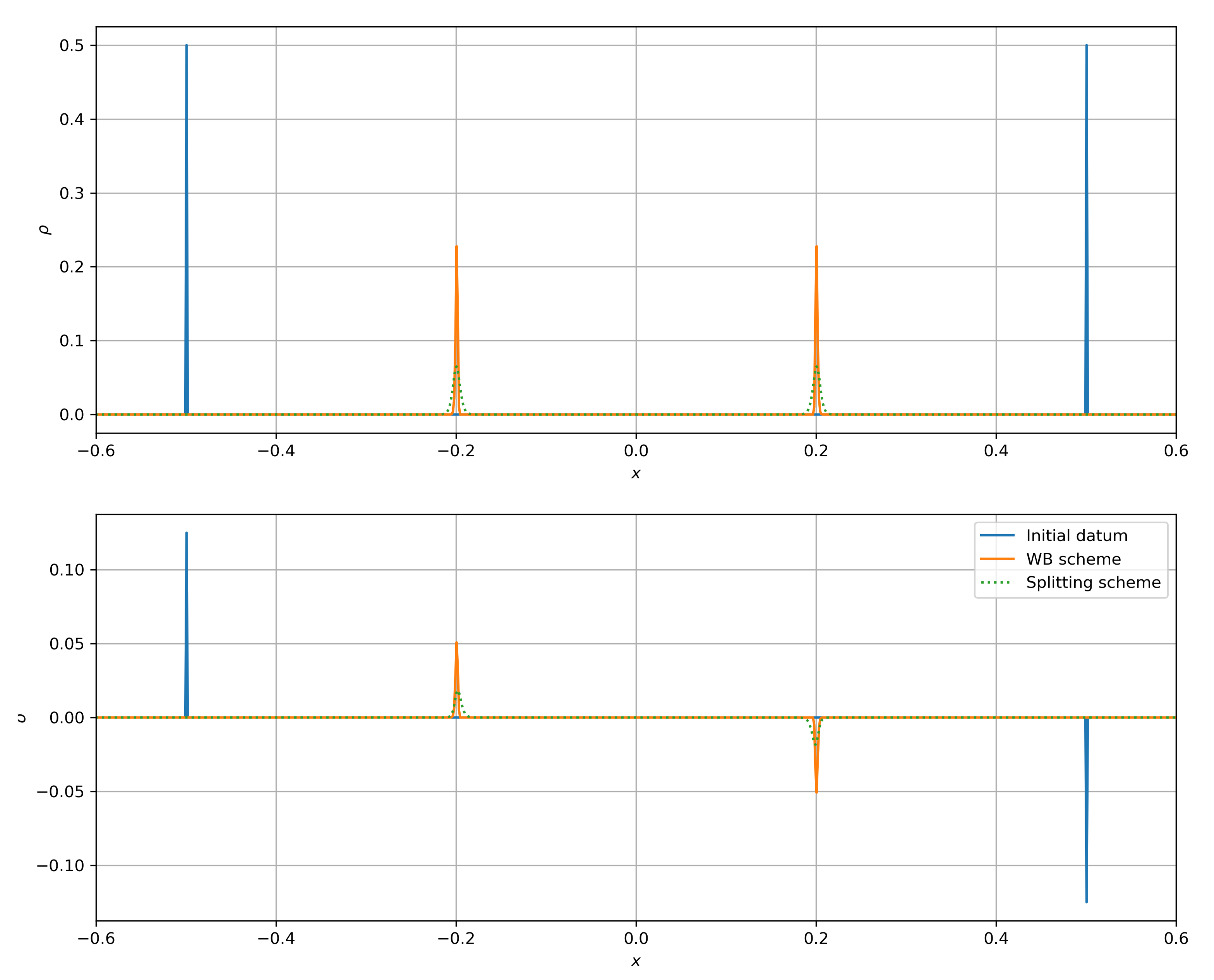
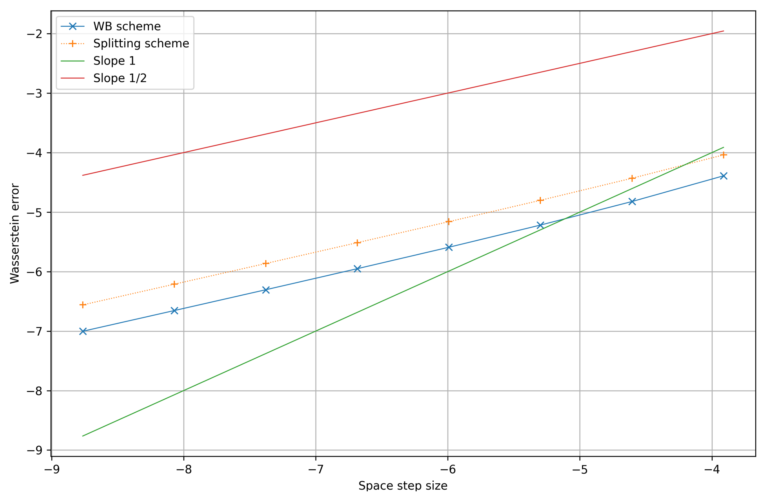
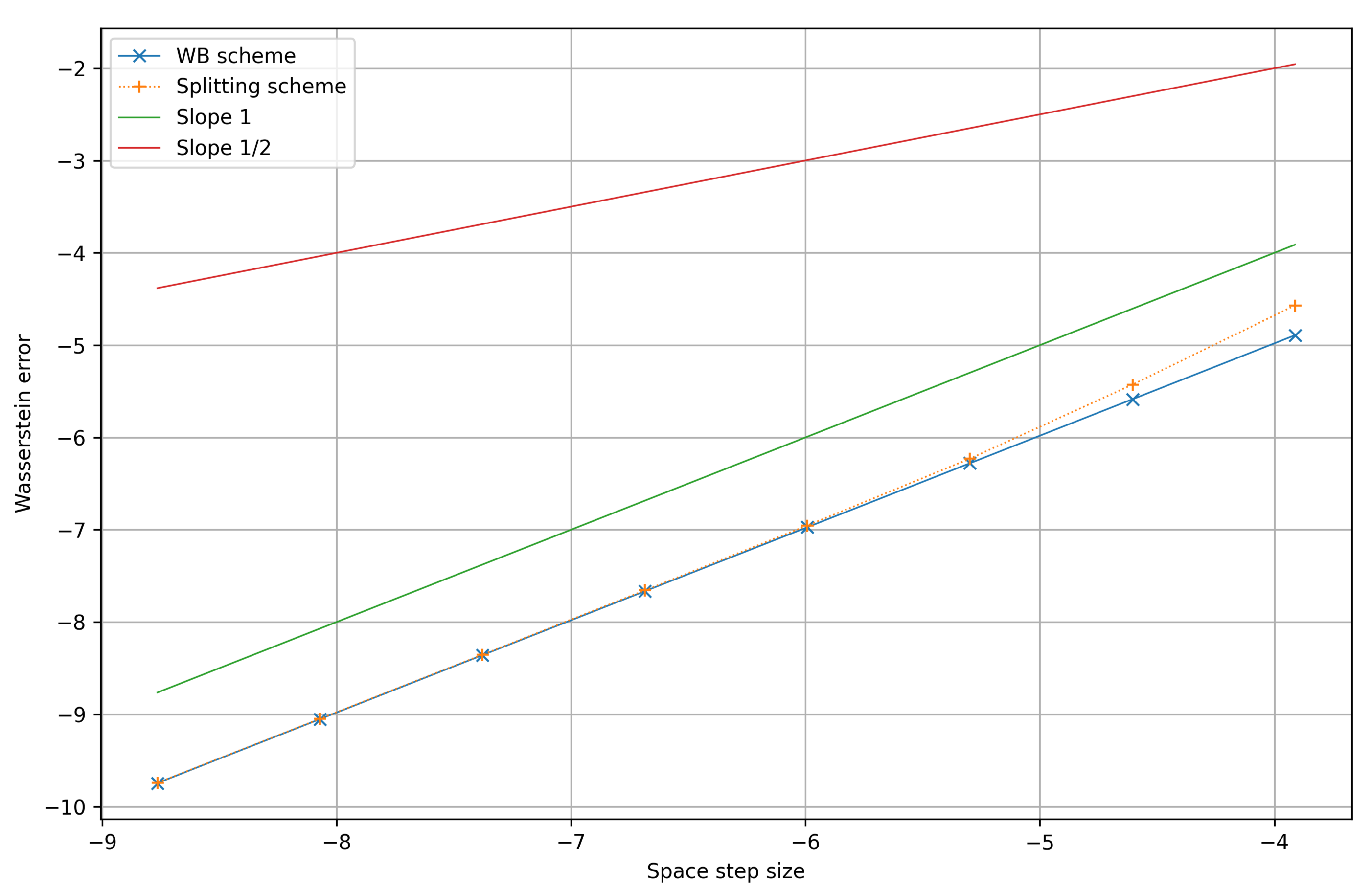
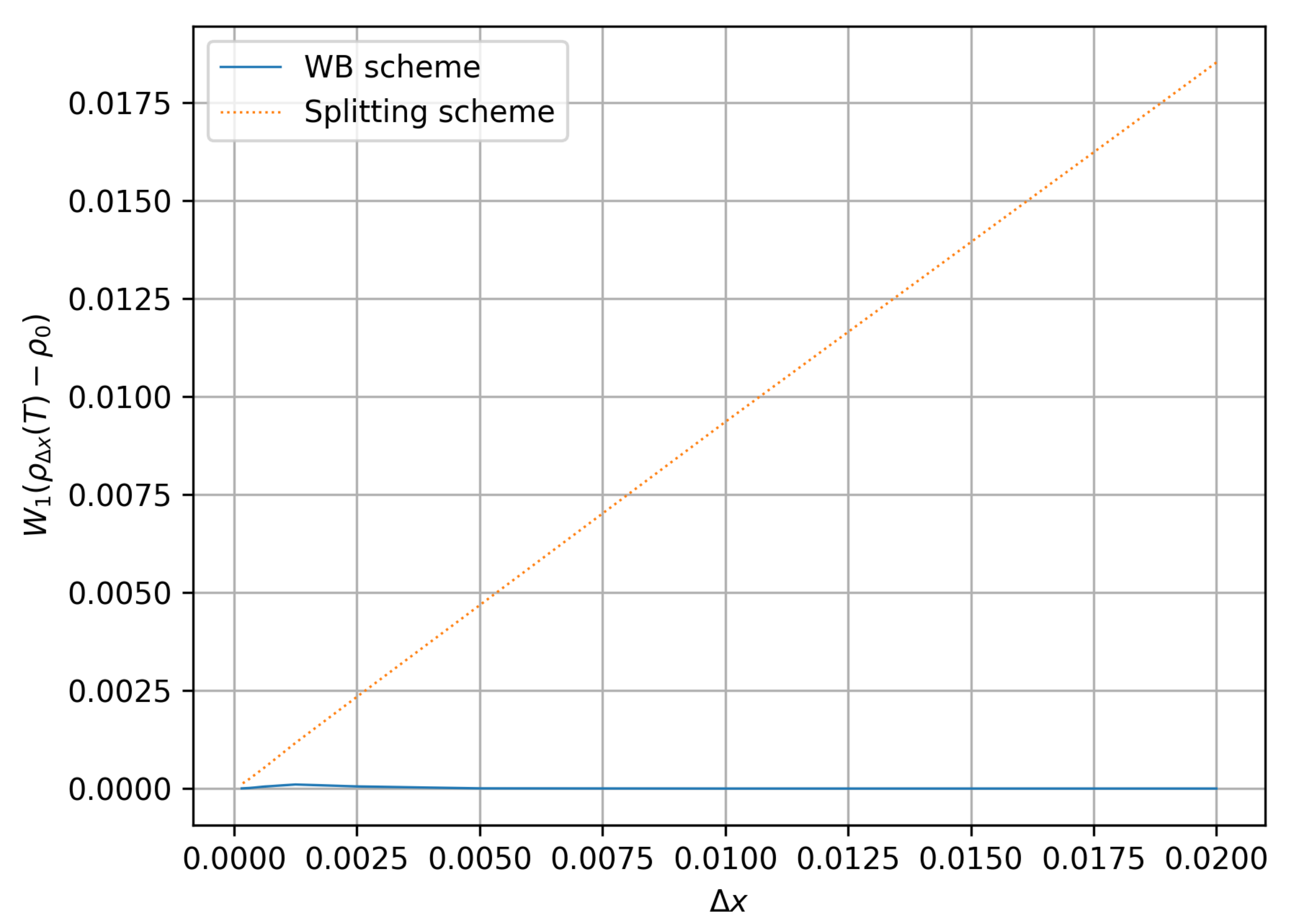
4. Numerical Experiments

We present some numerical illustrations for the two schemes described in the previous section. In addition to the potential $W\left(x\right)=\frac{\left|x\right|}{2}$, we also consider the smooth potential $W\left(x\right)=\frac{x^2}{2}$.

Numerical tests are conducted on the domain $[-1,1]$ with the inital data ${\rho }_0=\frac{1}{2}{\delta }_{-0.5}+\frac{1}{2}{\delta }_{0.5}$, ${\sigma }_0=a\left[{\rho }_0\right]{\rho }_0$ and both schemes are initialized with:

$${\rho }_j^0={\displaystyle \frac{1}{\Delta x}}{\rho }_0\left(C_j\right),{\sigma }_j^0={\displaystyle \frac{1}{\Delta x}}{\sigma }_0\left(C_j\right).$$

Figure 1 shows that both schemes recover the correct dynamics in the limit $\epsilon \to 0$: for the potential $W\left(x\right)=\frac{\left|x\right|}{2}$, one can compute the exact velocity of both Dirac masses for the aggregation Equation (1) and see that they should be located, respectively, in $x=-0.2$ and $x=0.2$ in final time $T=1.2$.

This test is set up with $\epsilon ={10}^{-7}$, on a Cartesian mesh of $[-1,1]$ with 1500 cells, $c=1$ and the CFL $c{\displaystyle \frac{\Delta t}{\Delta x}}=0.9$. Both schemes (27) and (49) display the correct velocity for the Dirac masses, but one can notice that the Rusanov scheme (27) shows more numerical diffusion. Note that both schemes are written in conservation form, they preserve the total mass of $\rho$, which is also verified numerically.

We then investigated the order of convergence when $\Delta x$ goes to 0 with $\epsilon$ fixed, in Wasserstein distance $W_1$ (the numerical results are the same for $W_2$).

After performing tests for several values of $\epsilon$, it appears that the convergence rate does not depend on the size of $\epsilon$. Therefore, as an example, we propose simulations in final time $T=0.5$, with the same intial data and stability parameters as above, and with $\epsilon =2\times {10}^{-6}$ for Figure 2 and with $\epsilon ={10}^{-2}$ for Figure 3:

For a fixed value of $\epsilon$, both schemes seem to converge with order $1/2$ with respect to $\Delta x$ for the smooth potential $W\left(x\right)=\frac{x^2}{2}$ (see Figure 2) whereas they seem to be of order 1 for the potential $W\left(x\right)=\frac{\left|x\right|}{2}$ (see Figure 3). This can be explained as both schemes possess some numerical diffusion which is somehow counterbalanced by the aggregation phenomenon in the case of a pointy potential, as already observed in [21]. Due to the link with the Burgers equation, this superconvergence phenomenon is directly linked to the results of Després [33], which should be rigorously extended to our case (the mere extension to the upwind scheme of [11] for the aggregation is not straightforward).

Finally, we also verified the well-balanced property of the scheme (48) by computing the $W_1$ distance between the approximated solution at time $T=0.5$ and the stationary solution of (2) given by

$$\rho (t,x)={\rho }_0\left(x\right):=\frac{1}{8\epsilon c^2}\left(1-{tanh}^2\left(\frac{x}{4\epsilon c^2}\right)\right).$$

The test is conducted with $\epsilon =2\times {10}^{-4}$, with the exact boundary conditions given by the above formula, and for several values of $\Delta x$. As we show in Figure 4, the scheme (48) preserves well the above equilibrium for any $\Delta x$ (although we replaced the resolution of the systems (30) and (31) with linear systems, see (38)), while for the splitting scheme, we recover the linear convergence towards ${\rho }_0$ which is, in this case, the exact solution.

References

1. Morale, D.; Capasso, V.; Oelschläger, K. An interacting particle system modelling aggregation behavior: From individuals to populations. J. Math. Biol. 2005, 50, 49–66. [Google Scholar] [CrossRef]
2. Burger, M.; Di Francesco, M. Large time behavior of nonlocal aggregation models with nonlinear diffusion. Netw. Heterog. Media 2008, 3, 749–785. [Google Scholar] [CrossRef] [Green Version]
3. Burger, M.; Capasso, V.; Morale, D. On an aggregation model with long and short range interactions. Nonlinear Anal. Real World Appl. 2007, 8, 939–958. [Google Scholar] [CrossRef]
4. Topaz, C.M.; Bertozzi, A.L.; Lewis, M.A. A nonlocal continuum model for biological aggregation. Bull. Math. Biol. 2006, 68, 1601–1623. [Google Scholar] [CrossRef] [Green Version]
5. Topaz, C.M.; Bertozzi, A.L. Swarming patterns in a two-dimensional kinematic model for biological groups. SIAM J. Appl. Math. 2004, 65, 152–174. [Google Scholar] [CrossRef]
6. Dolak, Y.; Schmeiser, C. Kinetic models for chemotaxis: Hydrodynamic limits and spatio-temporal mechanisms. J. Math. Biol. 2005, 51, 595–615. [Google Scholar] [CrossRef] [PubMed]
7. James, F.; Vauchelet, N. Chemotaxis: From kinetic equations to aggregate dynamics. NoDEA Nonlinear Differ. Equ. Appl. 2013, 20, 101–127. [Google Scholar] [CrossRef] [Green Version]
8. Bertozzi, A.L.; Brandman, J. Finite-time blow-up of L-weak solutions of an aggregation equation. Commun. Math. Sci. 2010, 8, 45–65. [Google Scholar] [CrossRef] [Green Version]
9. Bertozzi, A.L.; Carrillo, J.A.; Laurent, T. Blow-up in multidimensional aggregation equations with mildly singular interaction kernels. Nonlinearity 2009, 22, 683–710. [Google Scholar] [CrossRef] [Green Version]
10. Carrillo, J.A.; Difrancesco, M.; Figalli, A.; Laurent, T.; Slepčev, D. Global-in-time weak measure solutions and finite-time aggregation for nonlocal interaction equations. Duke Math. J. 2011, 156, 229–271. [Google Scholar] [CrossRef] [Green Version]
11. Carrillo, J.A.; James, F.; Lagoutière, F.; Vauchelet, N. The Filippov characteristic flow for the aggregation equation with mildly singular potentials. J. Differ. Equ. 2016, 260, 304–338. [Google Scholar] [CrossRef] [Green Version]
12. Jin, S.; Xin, Z. The relaxation schemes for systems of conservation laws in arbitrary space dimensions. Commun. Pure Appl. Math. 1995, 48, 235–276. [Google Scholar] [CrossRef]
13. James, F.; Vauchelet, N. Numerical methods for one-dimensional aggregation equations. SIAM J. Numer. Anal. 2015, 53, 895–916. [Google Scholar] [CrossRef] [Green Version]
14. Bonaschi, G.A.; Carrillo, J.A.; Di Francesco, M.; Peletier, M.A. Equivalence of gradient flows and entropy solutions for singular nonlocal interaction equations in 1D. ESAIM Control Optim. Calc. Var. 2015, 21, 414–441. [Google Scholar] [CrossRef] [Green Version]
15. James, F.; Vauchelet, N. Equivalence between duality and gradient flow solutions for one-dimensional aggregation equations. Discret. Contin. Dyn. Syst. 2016, 36, 1355–1382. [Google Scholar]
16. Katsoulakis, M.A.; Tzavaras, A.E. Contractive relaxation systems and the scalar multidimensional conservation law. Commun. Partial. Differ. Equ. 1997, 22, 225–267. [Google Scholar] [CrossRef]
17. Jin, S. Efficient asymptotic-preserving (AP) schemes for some multiscale kinetic equations. SIAM J. Sci. Comput. 1999, 21, 441–454. [Google Scholar] [CrossRef]
18. Carrillo, J.A.; Chertock, A.; Huang, Y. A finite-volume method for nonlinear nonlocal equations with a gradient flow structure. Commun. Comput. Phys. 2015, 17, 233–258. [Google Scholar] [CrossRef]
19. Craig, K.; Bertozzi, A.L. A blob method for the aggregation equation. Math. Comput. 2016, 85, 1681–1717. [Google Scholar] [CrossRef] [Green Version]
20. Gosse, L.; Vauchelet, N. Numerical High-Field Limits in Two-Stream Kinetic Models and 1D Aggregation Equations. SIAM J. Sci. Comput. 2016, 38, A412–A434. [Google Scholar] [CrossRef] [Green Version]
21. Fabrèges, B.; Hivert, H.; Le Balc’h, K.; Martel, S.; Delarue, F.; Lagoutière, F.; Vauchelet, N. Numerical schemes for the aggregation equation with pointy potentials. ESAIM Proc. Surv. 2019. [Google Scholar] [CrossRef]
22. Carrillo, J.A.; Fjordholm, U.S.; Solem, S. A second-order numerical method for the aggregation equations. Math. Comput. 2021, 90, 103–139. [Google Scholar] [CrossRef]
23. Gosse, L. Computing Qualitatively Correct Approximations of Balance Laws. Exponential-Fit, Well-Balanced and Asymptotic-Preserving; Springer: Milano, Italy, 2013; Volume 2, p. 340. [Google Scholar]
24. Villani, C. Topics in Optimal Transportation; American Mathematical Society (AMS): Providence, RI, USA, 2003; Volume 58, p. 370. [Google Scholar]
25. Santambrogio, F. Optimal Transport for Applied Mathematicians. Calculus of Variations, PDEs, and Modeling; Birkhäuser/Springer: Cham, Switzerland, 2015; Volume 87, p. 353. [Google Scholar]
26. Vallender, S.S. Calculation of the Wasserstein Distance Between Probability Distributions on the Line. Theory Probab. Appl. 1974, 18, 784–786. [Google Scholar] [CrossRef]
27. Rachev, S.T.; Rüschendorf, L. Mass Transportation Problems. Vol. 1: Theory. Vol. 2: Applications; Springer: New York, NY, USA, 1998; p. 430. [Google Scholar]
28. Natalini, R. Convergence to equilibrium for the relaxation approximations of conservation laws. Commun. Pure Appl. Math. 1996, 49, 795–823. [Google Scholar] [CrossRef]
29. Serre, D. Systems of Conservation Laws 1: Hyperbolicity, Entropies, Shock Waves; Cambridge University Press: New York, NY, USA, 1999. [Google Scholar]
30. Bouchut, F.; Perthame, B. Kružkov’s Estimates for Scalar Conservation Laws Revisited. Trans. Am. Math. Soc. 1998, 350, 2847–2870. [Google Scholar] [CrossRef] [Green Version]
31. Liu, H.; Warnecke, G. Convergence Rates for Relaxation Schemes Approximating Conservation Laws. SIAM J. Numer. Anal. 2000, 37, 1316–1337. [Google Scholar] [CrossRef] [Green Version]
32. Delarue, F.; Lagoutière, F.; Vauchelet, N. Convergence analysis of upwind type schemes for the aggregation equation with pointy potential. Ann. Henri Lebesgue 2020, 3, 217–260. [Google Scholar] [CrossRef] [Green Version]
33. Després, B. Discrete Compressive Solutions of Scalar Conservation Laws. J. Hyper. Differ. Equ. 2004, 01, 493–520. [Google Scholar] [CrossRef]
Figure 1. Dynamics of two Dirac masses for the potential W ( x ) = | x | 2 in time T = 1.2 .
Axioms 10 00108 g001
Figure 2. Order of convergence of the splitting scheme and the well-balanced scheme for the smooth potential W ( x ) = x 2 2 .
Axioms 10 00108 g002
Figure 3. Order of convergence of the splitting scheme and the well-balanced scheme for the pointy potential W ( x ) = | x | 2 .
Axioms 10 00108 g003
Figure 4. Distance to the equilibrium for the splitting scheme and the well-balanced scheme and for the pointy potential W ( x ) = | x | 2 .
Axioms 10 00108 g004
Publisher’s Note: MDPI stays neutral with regard to jurisdictional claims in published maps and institutional affiliations.