Estimation Algorithm for a Hybrid PDE–ODE Model Inspired by Immunocompetent Cancer-on-Chip Experiment

Abstract

The present work is motivated by the development of a mathematical model mimicking the mechanisms observed in lab-on-chip experiments, made to reproduce on microfluidic chips the in vivo reality. Here we consider the Cancer-on-Chip experiment where tumor cells are treated with chemotherapy drug and secrete chemical signals in the environment attracting multiple immune cell species. The in silico model here proposed goes towards the construction of a “digital twin” of the experimental immune cells in the chip environment to better understand the complex mechanisms of immunosurveillance. To this aim, we develop a tumor-immune microfluidic hybrid PDE–ODE model to describe the concentration of chemicals in the Cancer-on-Chip environment and immune cells migration. The development of a trustable simulation algorithm, able to reproduce the immunocompetent dynamics observed in the chip, requires an efficient tool for the calibration of the model parameters. In this respect, the present paper represents a first methodological work to test the feasibility and the soundness of the calibration technique here proposed, based on a multidimensional spline interpolation technique for the time-varying velocity field surfaces obtained from cell trajectories.

1. Introduction

Recruitment of immune cells to a tumor is a key parameter in cancer prognosis and response to therapy and the complex relationship between cellular, noncellular components and secreted chemotactic factors plays an essential role in directing the migration of both activating and suppressive immune cell types. In recent years with the development of the highly multidisciplinary Organ-on-Chip field (OOC) [1,2], microfluidic technologies are employed as valuable in vitro platform tools to build tumor microenvironments, with modular degree of complexity and to visualize and quantify immune infiltration in response to anticancer therapies.

The work that set the stage for Organs-on-Chip (OOC) was published in 2010 [3] and thereafter OOC constituted a dynamic field of research, and substantial effort has been devoted to creating realistic mimics of different organs in recent years [4,5,6,7].

The coupling with live-cell imaging may enable extraction of single-cell tracking profiles which can be processed with advanced mathematical tools. In this context, the present study is inspired by the modeling of the complex mechanisms behind the cell dynamics and interactions between immune (ICs) and treated tumor (TCs) cells in microfluidic chips. In this framework, several studies [1,7,8] were conducted on immunocompetent cancer-on-chips to assess the effects of therapeutic drugs on TCs and on the possible reactions of the immune system. One of the first studies addresses the role of formyl peptide receptor 1/annexin a1 axis in anti-tumor response to anthracycline-based chemotherapy [7]. Timelapse recordings were performed in a microfluidic platform designed for oncoimmunology [1] research to assess physical and chemical contacts between malignant and immune populations. Some of the earliest applications of microfluidic cell culture technology focused on modeling specific steps in the cancer cascade, including tumor growth [9] and expansion [10], angiogenesis [11,12,13,14,15,16], progression from early to late stage lesions involving an epithelial–mesenchymal transition [17,18], tumor cell invasion [19] and metastasis [20]. Although Organs-on-Chip represent an increasing in importance field of research because it allows experimentalists to have major control on the objects of investigation, resulting in more accurate measurements, some aspects still remain difficult to understand. In particular, a quantification of the average chemical gradients present in the chip environment is difficult to be estimated.

Motivated by these laboratory experiments, we present an in silico mathematical model to describe ICs migration in the case of an efficient interaction with TCs treated with chemotherapeutic drug.

The main goal of this work is to build a bridge between experimental data coming from Cancer-on-Chip experiment given as particles and macroscopic mathematical models, such as the one proposed in reference [21], in order to gain further insights on the dynamics and short-range interactions between cells. Indeed, the present works goes towards the direction of the mean-field limit to unveil the statistical properties of the model. Recently, one of the authors of the present paper has derived rigorously in Wasserstein’s type topologies the mean-field limit (and propagation of chaos) to the Vlasov-type equation, in the framework of generalizations of the kinetic model given by Cucker–Smale dynamical system, see reference [22]. Here we propose a simulation algorithm based on a hybrid macroscopic-microscopic chemotaxis model able to reproduce the main features of phenomena observed in microfluidic chip, such as migration of ICs and short-range interactions with cancer cells representing the sources of chemical gradients.

Existing methods used in the literature so far were dealing with the description of particle trajectories and are essentially represented by statistics on cell trajectories, as in the work by Agliari et al. [23]. Another possibility, already applied in other papers dealing with particle trajectories, see for instance reference [24], is to compute the distance between immune cells and tumor cells across time. However, we would like to stress that here our main concern is to show the feasibility of the proposed approach and to create a connection with macroscopic modeling of the same problem, in order to see what happens when we go to the limit (corresponding to the situation in which millions of cells move in the environment). Our final aim is indeed to be able in the future to simulate the behavior of immune cells in the tissue of an organ. In this framework, a novel strategy for the estimation of model parameters to perform the validation against real data and the calibration of the mathematical model is introduced. Such strategy involves from one hand the analysis of ICs trajectories coming from experimental data to describe realistically the average speed and the pathways of immune cells and the creation of a synthetic dataset for evaluating the effectiveness of the calibration technique for the estimation of model parameters. Moreover, in order to determine the velocity distribution of ICs, a stochastic component is obtained analyzing real trajectories of cells falling in the area under examination and then it is added to the deterministic velocity field.

The modeling of dynamics and interactions in microfluidic chip environment was already studied in [18,25,26,27] with particle models and with cellular automata models in [28]. In [21] a fully macroscopic mathematical (PDE) model was considered, both for the chemical gradient which is seen as an average field and for the density of immune cells. With the PDE model we were able to describe long-range interactions in the chip environment and a first estimate of the chemical gradient driving ICs movement was obtained in [29].

Here, instead, we are interested in describing efficient short-range interactions between treated tumor cells and immune cells. As an example of this phenomenon, we considered the study and the experimental setting in [7], where tumor cells treated with chemotherapy drug release a chemical stimulus sensed by healthy immune cells, thus promoting their migration towards the tumor cells. For the construction of the model, we used a discrete in continuous approach where we coupled a reaction-diffusion partial differential equation (PDE) describing the evolution of the average substances released by the TCs in the tumor microenvironment with a particle model, where every IC in the system was considered to be a single entity and provided with specific properties, as previously done in [30] in a different experiment. Here the hybrid approach was revealed to be crucial in providing a proper description of the multiscale phenomenon that with a traditional macroscopic model would not be possible to fully decipher. In particular, our model describes the dynamics of each IC by means of ordinary differential equations (ODE) in such a way that every cell can be followed individually. Since the motion of ICs is driven by chemotaxis, the migratory activity is regulated by a chemotactic term which allows them to sense the gradient of the chemicals in the tumor neighborhood and of specific forces such as adhesion–repulsion which establish between cells.

The calibration of the mathematical model is supported by the development of ad-hoc parameter estimation procedure based on an interpolation technique for the approximation of the velocity field of ICs across time, i.e., multidimensional spline method previously introduced in [31] and described in Section 4.1. Such procedure, applied to synthetic cell trajectories dataset, provides accurate estimates for the values of unknown model parameters and demonstrates to be a promising approach for the validation of the proposed model against real data.

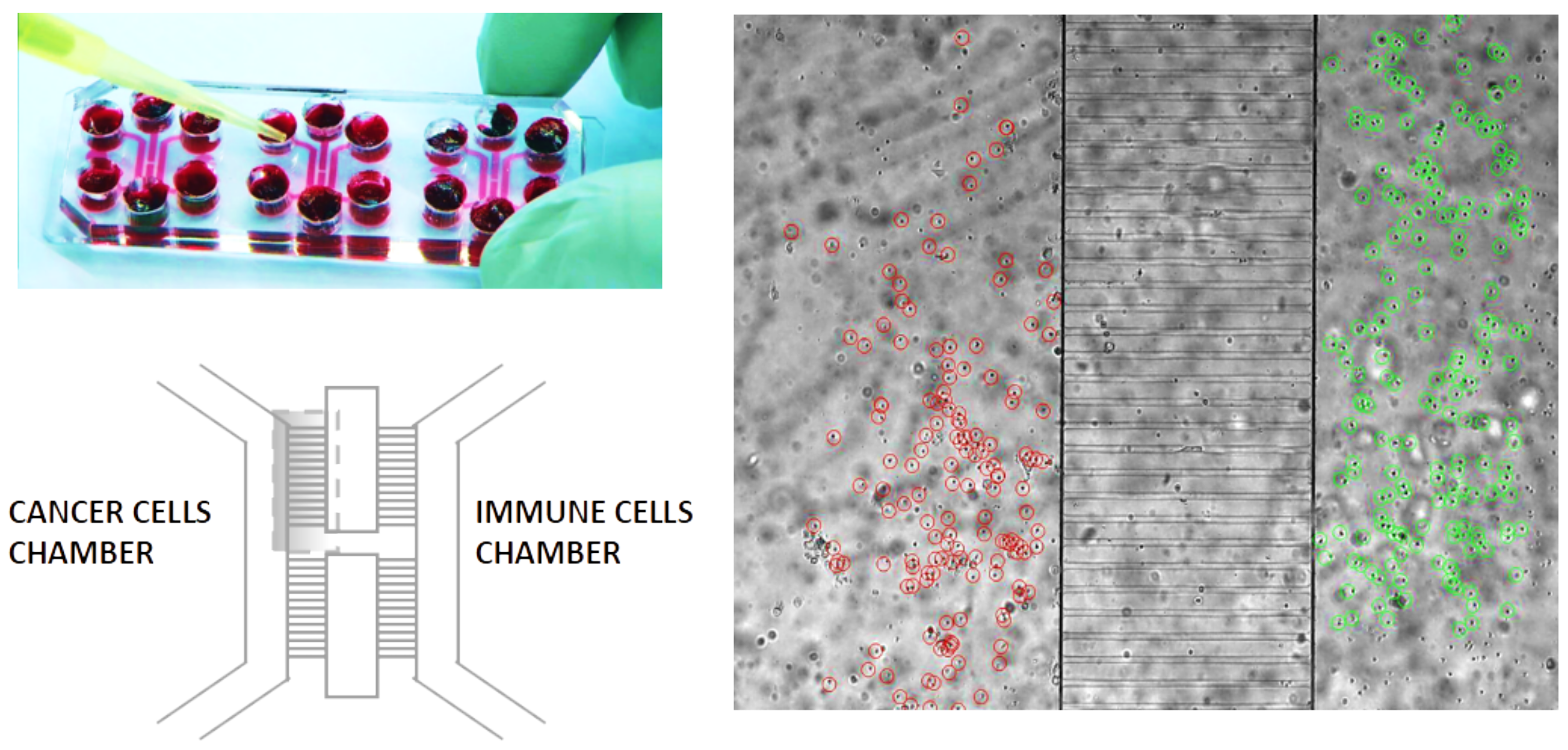
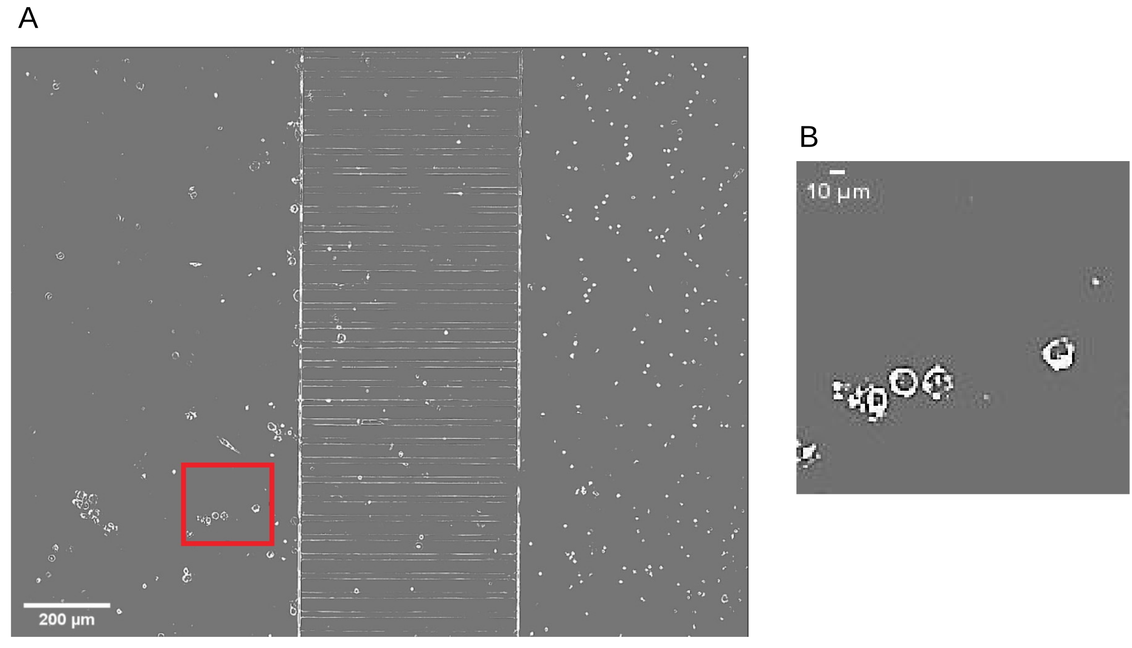
1.1. The Geometry of the Microfluidic Chip and the Related Computational Domain

The immune-oncology chip designed for the experiment consists of three main culture chambers for plating adherent TCs and floating ICs connected by a bridge of microcapillaries allowing chemical and physical contacts. In Figure 1 a picture of the two boxes is shown. With regards to the dimensions, the capillaries have, respectively, width and length of 12 $\mathsf{\mu }$$\mathrm{m}$ and 500 $\mathsf{\mu }$$\mathrm{m}$, while the height is of 10 $\mathsf{\mu }$$\mathrm{m}$; however, since in the video footage the experiment is recorded at a fixed height, the third spatial dimension in our framework is neglected.

The cross-sectional dimensions of culture chambers are 1 $\mathrm{m}$$\mathrm{m}$ (width) × 100 $\mathsf{\mu }$$\mathrm{m}$ (height). Further details about the chip design are illustrated in [7]. We also underline that here we are considering a 2D culture in the liquid with dying cancer cells adherent to the glass slide and mainly static, and immune cells floating.

In the experimental set-up, the timelapse observation area comprises left TCs culture chamber and central one with loaded ICs. Our goal consists of modeling the migration of ICs towards the TCs taking into account the different forces acting on the cells. To achieve such a result, we neglected the migration of ICs in the right chamber and through the microchannels, and we only focused on motility patterns of infiltrated ICs in the TCs left chamber.

Moreover, in order to better analyze the short-range dynamics and interactions between tumor and immune cells, we restricted our study on a subarea of the left chamber of length and height equal to 200 $\mathsf{\mu }$$\mathrm{m}$. This area corresponds to the subset $[400,600]\times [200,400]$ $\mathsf{\mu }$$\mathrm{m}$, and we defined it as $\Omega =[0,L_x]\times [0,L_y]$. In Figure 2 we present the setting of the experiment at time $t=24$ h, with a focus on the area under analysis. The main reason for considering only a portion of the chip is motivated by:

• the reduction of the computational cost in view of the optimization procedure for the parameter estimation;
• the focus on short-range interactions.

Moreover, $\Omega$ contains four treated TCs, and this makes the area a good representative of cell dynamics, since in the laboratory experiment there are about 60 TCs in the entire chamber.

1.2. Original Contribution of the Present Paper

To describe such complex mechanisms with a multiscale nature, the model here proposed belongs to the category of hybrid models, involving the coupling between macroscopic and microscopic models.

As mentioned above, we assume the presence of forces between cells, which are established due to the chemoattractant and due to the nature of the cells itself. For this reason, in the current work, we refer to the discrete–continuous model (1)–(2) proposed in [30] to describe the morphogenesis of the posterior lateral line system in zebrafish. Such a model includes a classical reaction-diffusion partial differential equation (PDE) used to describe the evolution of the concentration of chemicals released by TCs in the tumor milieu, coupled with ordinary differential equations (ODEs) for the inter-cellular dynamics of ICs, which establishes both due to the presence of the chemoattractant and to the forces generated between the cells. In particular, the use of a particle model permits the highlighting of the role of single cells in the space, to analyze short-range interactions and to attribute specific characteristics to cells behavior that a macroscopic model would not allow. As mentioned in Section 1.1, for computational reasons and for the datatype at our disposal, cell tracks extracted from video recorded at a fixed level on the z-axis, we neglect the third dimension and consider only the 2D case. However, the third dimension can be easily taken into account by the model, but we do not expect important changes in the overall dynamics.

Here, chemical signals are described as an average field by means of a reaction-diffusion equation

$${\partial }_{t}f=D\Delta f+S(t,\mathbf{Y},f)$$

(1)

with a possible source or degradation term given in S term. Equation (1) was endowed with Robin boundary conditions to state the exchange of chemicals between the internal and the external environment. The gradient field f influences the evolution of cell positions, according to a second order equation of the form:

$${\ddot{\mathbf{X}}}_i=F(t,\mathbf{X},\dot{\mathbf{X}},\mathbf{Y},f,\nabla f)-\mu {\dot{\mathbf{X}}}_i$$

(2)

where ${\mathbf{X}}_i$, $i=1,\dots ,N_{tot,I}$, is the position vector of the i-th IC, $N_{tot,I}$ is the total number of ICs, $\mathbf{X}=({\mathbf{X}}_1,\dots ,{\mathbf{X}}_{N_{tot,I}})$ contains all the positions, and $\dot{\mathbf{X}}=({\dot{\mathbf{X}}}_1,\dots ,{\dot{\mathbf{X}}}_{N_{tot,I}})$ the velocities. The vector $\mathbf{Y}=({\mathbf{Y}}_1,\dots ,{\mathbf{Y}}_{N_{tot,T}})$, $i=1,\dots ,N_{tot,T}$, stands for TCs positions, which are taken as constants in the problem, since dying TCs do not migrate as time evolves. The function $\mathbf{F}$ includes several effects: from the detection of the chemical signal f (chemotaxis) to mutual interactions between ICs (adhesion and repulsion) and ICs and TCs (adhesion and repulsion). All these effects take into account a non-local sensing radius. The term $\mu {\dot{\mathbf{X}}}_i$ represents damping due to cell adhesion to the substrate.

We remark that the use of second order equations to describe the cell motion was first used in the seminal work [32] in the framework of Newton’s equation of motion for particles. Indeed, even in this case the acceleration is not so high, this formulation describes the effects of the presence of an external force causing velocities and direction changes. Moreover, the friction term for cells immersed in a fluid is also taken into account. In order to have a more complete model able to represent the randomness characterizing cell motility, we also introduced a stochastic component in the velocity field in the spirit of Langevin model, see the review [33] and references therein.

In this context, in order to better reproduce the phenomenon under consideration such as the presence of chemical stimulus of treated cancer cells, we applied the following modification respect to the model in [30]:

• we model the presence of tumor cells, and we also take into account the repulsion forces to avoid overlapping. Eventually, a slight overlay may occur between tumor and immune cell in the case of close interactions. However, it does not seem to occur in the video footage;
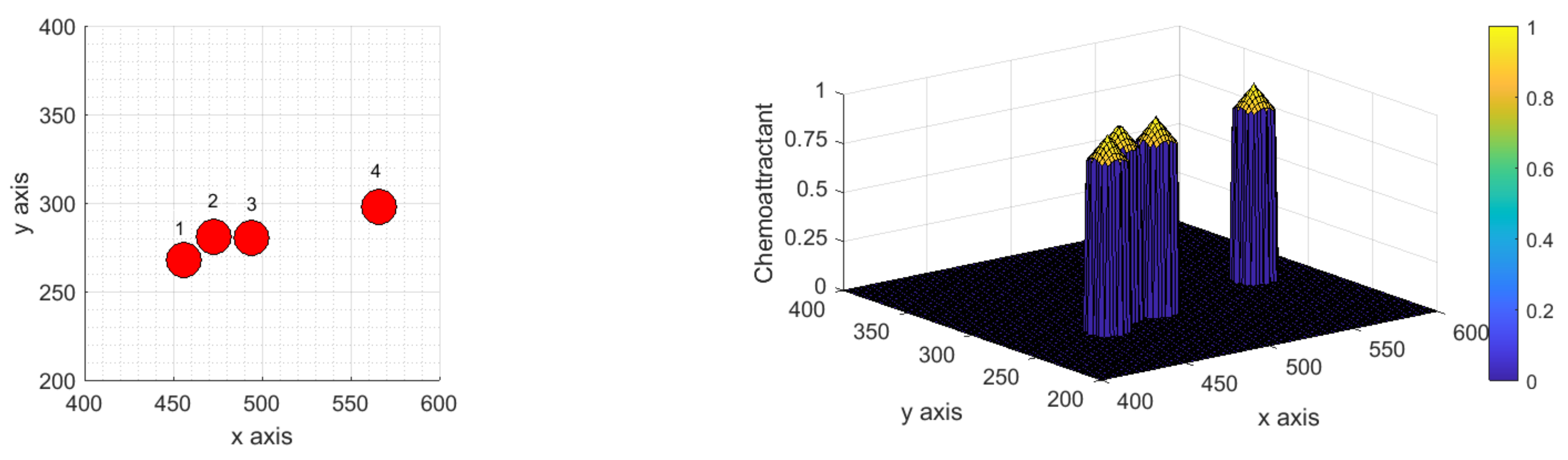
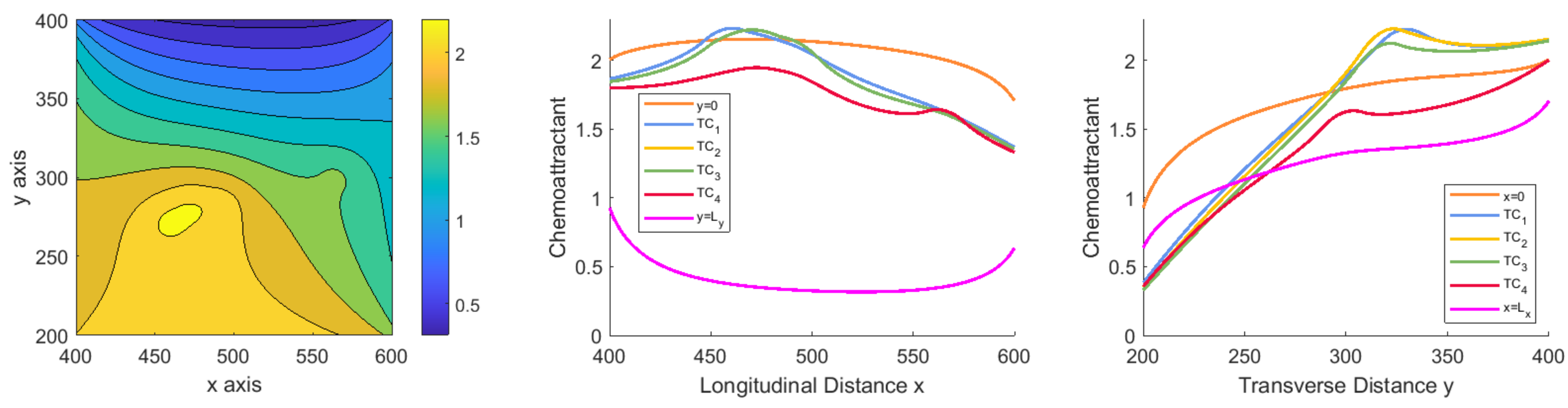
• a chemical gradient concentrated around sources represented by cancer cells is considered and diffused in the environment;
• Robin boundary conditions for the inflow of chemoattractant in the area under consideration are applied and adjusted to drive cell migration in a diagonal direction, as observed experimentally;
• the alignment effect between cells is discarded since in this context is not present;
• a chemotactic sensitivity term—i.e., receptor saturation—is added in the drift term of the equation of particles motion, with the effect that chemotaxis of cells is reduced in areas of high chemoattractant concentrations;
• a stochastic component in the particle velocities is added to have more realistic cell trajectories in terms of randomness.

The equations are solved in a square domain $\Omega$, introduced in Section 1.1, subset of the chamber where the experiment was performed and the approximation was carried out using a classical central difference scheme in space and the Crank–Nicolson scheme in time, although in Appendix A we prefer to present the general form of the scheme based on the $\theta$-method.

The main novelty of our approach here is mainly represented by:

• the modeling study on ICs behavior by considering different scenarios, see Section 3;
• the construction of a calibration algorithm to find a trustable estimate of the most significant parameters of the model to assess the effects of chemical gradients on the ICs movement, see Section 4.

In particular, such calibration algorithm—based on the mathematical model—is built to test the possibility of validating the model on real data provided by experimentalists. The main goal of the present work is indeed the introduction of a robust procedure for the estimate of model parameters by means of the paths taken by ICs in the chip subarea under examination. It is worth noting that this is not an easy task, since to succeed in the model calibration we need to extract a common behavior from the time-varying trajectories of immune cells located at different points of the examined area. For this reason, in this first work based on this framework we propose a calibration strategy taking into account this variability and applying it to a synthetic dataset, in order to assess the effectiveness of our methodology.

We underline that the synthetic dataset of ICs pathways has been created reproducing qualitatively the real trajectories extracted from the video footage of the experiment, in order to have a "realistic" dataset. In more detail, a set of trajectories of cells sharing an average behavior has been produced by suitably tuning model parameters to have an upper and lower bound of cell speeds taken from the experimentally observed ones. With these synthetic trajectories, we have computed ICs velocity field at every observation time as a surface produced by the model itself, supposing to have a single population of immune cells thus showing an average behavior. Such velocity field has been then approximated using a multidimensional spline interpolation technique, described in Section 4.1 to have smoothing in time and space on the dataset to be compared.

Finally, this average field has been used as our target solution to be used in the calibration procedure, as described in detail in Section 4.2. The methodology for the error quantification is based on the minimization of a cost functional depending on the difference between the target velocity field of cell in the whole domain and the velocity field obtained for another choice of the model parameters during the optimization procedure performed with a local search method and we compared them at every time step. In addition to this, we also studied the introduction of further terms in functionals with the aim of improving the optimization results and show the soundness of our algorithm representing a starting point for investigations on experimental data in the next future.

1.3. Main Contents and Plan of the Paper

We introduce a hybrid model composed of a reaction diffusion equation, describing the time and space evolution of signaling substances released by treated TCs in a subarea of the main chamber, and of an agent-based model made up of second order differential equations for each IC. The boundary conditions associated with the partial differential equation are of Robin type, so that we can have a control on the amount of chemical exchanged with the surrounding microenvironment. In addition, based on experimental observation, an ad hoc parameter estimation technique was developed. To summarize the main contents of the present work, the mathematical issues faced in this study are identified into:

• the development of a mathematical model describing the behavior of ICs in short-range interactions in the microfluidic chip environment;
• the development of ad-hoc parameter estimation techniques for time-varying velocity fields.

The plan of the paper is as follows. In Section 2 we describe the biological framework that inspired our study, and we introduce the mathematical formulation of biologically inspired models, and we present the adopted model. Section 3 is devoted to the modeling study on the scenarios suggested from the observation of the dynamics in the laboratory experiment performed with the numerical simulation algorithm reported in the Appendix. Section 4 contains the parameter estimation techniques here developed and the results obtained with the calibration algorithm. A sensitivity analysis is also performed and reported in the Appendix. Finally, in Section 5 we discuss the presented results, and the future aims of our work.

2. Materials and Methods

2.1. Biological Framework

The OOC technology allow the design and recreation of more sophisticated in vitro cellular microenvironments under physiological or pathological scenarios; as potential candidates for better prediction of human responses than animal testing cannot. This success is also due thanks to compatibility with a variety of microscopy techniques including live-cell high-content imaging and to the wide variety of cells and tissues that the chips can host, see [1].

One of the most challenging scenarios for the application of these devices is represented by cancer-immune relations due to very complex and not still completely discovered signaling modalities between ICs and TCs. Some attempts have been presented with the aim of modeling the effect of drugs on TCs, see for instance [34,35] where the microfluidic devices helped to control and evaluate the magnitude of cancer responses.

In particular, here we refer to the study in Vacchelli et al. [7], where timelapse imaging of microfluidic co-cultures were performed to investigate the motility patterns and crosstalk between ICs and TCs in the context of chemotherapy-induced anticancer immune responses.

Setting of the Laboratory Experiments

Details on the in vitro microfluidic experiments, type of cells involved and loading procedures can be found in [7,36]. Briefly, human breast cancer cells were previously treated with anthracycline-based chemotherapy and were cultivated in the left chamber. This treatment triggers the process of immunogenic cell death [37], according to which TCs release danger signals. The right chamber is loaded with unlabeled human peripheral blood mononuclear cells (PBMCs) from healthy donors (with normal expression of FPR1). PBMCs start migrating biased by the detection of chemical signal produced by TCs and after crossing microchannels enter in contact with dying cancer cells, engaging in stable interactions leading to TCs killing events.

In the chip, the chosen culture medium is neutral, which means that no exogenous substance is introduced. Timelapse imaging was performed using a microscope placed directly inside the CO${}_2$ incubator for all the duration of the recordings. Images were taken every 2 min over a period of 72 h of migration. Immune cells tracks (<400) were extracted in left chamber (interval time: 24–48 h) using TrackMate plugin(ref) available in the Fiji/ImageJ software (https://imagej.nih.gov/ij/, accessed on 1 August 2020).

Our aim consists of designing a basic mathematical model able to capture the main aspects related to the migratory movement of the ICs with respect to TCs. Therefore, we only focus on the case of efficient interaction between dying cancer cells exposed to ICD inducers and immune cells from healthy donors. Concurrently, we want to develop an algorithmic calibration procedure to derive model parameter values as close to empirical observations as possible.

2.2. Mathematical Framework

In this context, it is important to remark that late years have experienced an increasing interest in the direction of developing techniques to combine experimental data and mathematical models, in order to produce systems, i.e., in silico models, whose solutions could be as close as possible to the experimental outcomes. Indeed, the success of informed models is mainly due to the consistent improvements in computational abilities of the machines and in imaging techniques that allowed a wider access to data.

The involvement of the immune system in all stages of the tumor life cycle, including prevention, maintenance and response to therapy is now recognized as central to understanding cancer development from a systemic point of view. The increasing availability of experimental data and of treatment options, have represented a breeding ground to construct always more precise models. From a mathematical point of view, equations of different nature can be considered, depending on the type of analysis to be carried out. In macroscopic models, consisting of PDEs, any reference to the single constituents, the cells, are neglected, and macroscopic quantities such as the average cell densities are taken into consideration, see for instance the classical models [38,39] and their application to the immunocompetent microfluidic chip experiments in the recent work [21], allowing the simulation of long-range dynamics of immune cells driven by the chemical gradients secreted by cancer cells in the environment. The evolution of chemical stimuli in the tumor microenviroment can be also described by means of ODE models, see for instance the work [25] consisting of three ODEs that model the dynamics of effector and tumor cells and the cytokine IL-2, is one of the first to describe tumor-immune cells interactions. Another model in the same direction is due to Lee et al. [18], where changes in velocity and directionality of ICs are modeled with a system of ODE considering the combined effects of the interstitial flow, the tumor mass, the cytokines IL-8 and CCL-2, and the related receptors. Moreover, ODE models describing cell responses heterogeneity to death ligand (cytotoxic drugs) observed in laboratory experiments with single-cell techniques is proposed in [40]. In [28] the immune system is depicted as a network in the framework of cellular automata, where the nodes are molecules and cells and the arches connecting them are the influences each node has on others. Another kind of modeling consists of combining the macro approach expressed by a PDE, with the micro approach expressed by an ODE.

Hybrid models, developed including the macroscopic and microscopic scales, have been deeply studied in recent years, see [41,42,43,44]. In particular, in [41] a hybrid discrete–continuous model of metastatic cancer cell migration was developed, while in [45] a hybrid discrete-continuum approach was applied to model Turing pattern formation. In [43] a 3D agent-based model is proposed using an off-lattice approach to simulate vasculogenesis. For a comprehensive literature review of hybrid models sees the book chapter [46].

Here, in the framework of hybrid deterministic PDE–ODE models, we propose a discrete–continuous approach previously applied in [30], where immune cell motion is governed by ODE and the diffusion of chemoattractant released by cancer cells in the environment is described by PDE. The present work is complementary to the fully macroscopic approach proposed in [21], since it allows a zooming on immune system dynamics. Moreover, we enriched the equations of cell motion with a Brownian component to reproduce zigzag pathways of ICs.

The Model

Here we develop a model that can mimic cell migration under the effects of chemicals released by TCs on immune system dynamics. The considered TCs are experiencing apoptosis during which they liberate damaged-associated molecular patterns together with tumor antigens that elicit an immune response. For the sake of simplicity, the alarm concentrations are not differentiated, and we indicate them by means of the chemoattractant f, whose evolution is described by a PDE. At the cellular level, the model is discrete and includes the equation of the motion of each IC. We also underline that since we refer to experiment of treated cancer cells, according to the experimental setting we do not need to include TCs migration or duplication in our model. Let us summarize the main ingredients which compose the model.

For the IC motion we use a second order dynamic equation, which takes into account the forces acting on the cells that arise from the presence of the chemical signals and from the mechanical interactions between cells. The effect of cancer is described by a chemotactic term produced by the gradient of the f. The cell–cell mechanical interactions due to filopodia, consist of a radial attraction and repulsion depending on the relative positions of the cells, see [47] for experimental results in this direction. To describe this effect we refer to the mechanism introduced in [48]. The action of ICs regarding TCs is described by a radial repulsion term, depending on cells positions. Finally, we introduce a damping term, proportional to the velocities, which models cell adhesion to the substrate [49,50,51].

About the concentration of the chemoattractant, we associate a diffusion equation including a source term, given by the chemoattractant released by TCs, and a natural degradation term.

In the current context, the species under examination are TCs and ICs, but we underline that the setting can be made more complex with the introduction of a greater number of cell species and with the presence of an exogenous substance in the environment. Furthermore, in the present framework we are not taking into account the killing activity of ICs towards TCs as we already did in [21], since we do not have a quantitative data regarding the killing rate of immune cells in the chip environment. However, in the future also this feature will be included in the model.

Let ${\mathbf{X}}_i$ be the position of the i-th IC and $f(\mathbf{x},t)$ the total chemoattractant concentration, the following equations are introduced:

$$\{\begin{array}{cc}{\partial }_{t}f=D\Delta f+\xi F_4\left(\mathbf{Y}\right)-\eta f\hfill & \text{(3)}\hfill \\ {\ddot{\mathbf{X}}}_i=\gamma F_1(\chi \left(f\right)\nabla f)+F_2\left(\mathbf{X},\mathbf{Y}\right)+F_3\left(\mathbf{X}\right)-\mu {\dot{\mathbf{X}}}_i\hfill & \text{(4)}\hfill \end{array}$$

where $\gamma$, $\mu$, $\xi$ and $\eta$ are given constants and $F_n(·)$, $n=1,2,3,4$ are suitable functions.

Function $F_1$

The term $F_1$ is the chemotactic term and therefore it is related to the detection of a chemical signal by i-th cell in its neighborhood and it is taken to be a weighted average over a ball of radius $\overline{R}$ and centered in ${\mathbf{X}}_i$:

$$F_1\left(g(\mathbf{x},t)\right)={\displaystyle \frac{1}{\mathcal{W}}}{\int }_{\mathbf{B}({\mathbf{X}}_i,\overline{R})}g(\mathbf{x},t)w_i\left(\mathbf{x}\right)d\mathbf{x},$$

(5)

where

$$\mathbf{B}({\mathbf{X}}_i,\overline{R}):=\{\mathbf{x}:||\mathbf{x}-{\mathbf{X}}_i\left|\right|\le \overline{R}\},$$

$\parallel ·\parallel$ being the Euclidean norm,

$$w_i\left(\mathbf{x}\right)=\left\{\begin{array}{cc}2exp\left(-\left|\right|\mathbf{x}-{\mathbf{X}}_i{\left|\right|}^2{\displaystyle \frac{log2}{{\overline{R}}^2}}\right),\hfill & \mathrm{if}\left|\right|\mathbf{x}-{\mathbf{X}}_i\left|\right|\le \overline{R},\hfill \\ 0,\hfill & \mathrm{otherwise},\hfill \end{array}\right.$$

(6)

is a truncated Gaussian weight function, and

$$\mathcal{W}:={\int }_{\mathbf{B}({\mathbf{X}}_i,\overline{R})}{w}_i\left(\mathbf{x}\right)d\mathbf{x},$$

independently on i. A similar definition holds for the vector quantity $F_1$.

In addition, the function $F_1$ contains the gradient of the chemical substance and a chemotaxis function $\chi \left(f\right)$, representing the chemotactic sensitivity of ICs. Such chemotactic function, suggested in [52] by Lapidus and Schiller (1976) has the form:

$$\chi \left(f\right)={\displaystyle \frac{k_1}{{(k_2+f)}^2}},$$

(7)

where $k_1$ represents the cellular drift velocity, while $k_2$ is the receptor dissociation constant, which indicates how many molecules are necessary to bind the receptors. Such function is known as receptor saturation function and has the effect of reducing chemotaxis of cells in areas of high chemoattractant concentrations. In the integral, $\overline{R}$ will be chosen larger than the IC radius $R_I$, thus relation (5) describes a chemical signal that is sensed more in the center of the cell and less at the edge of the cell extensions.

Function $F_2$

Function ${\mathbf{F}}_2$ includes a repulsion effect among TCs and ICs. In particular, repulsion occurs at a distance between the centers of two cells less than $R_1$, where $R_1$ is defined as the sum of the two radii, $R_I$ and $R_T$, of the immune and tumor cells, respectively. With this formulation, repulsion occurs when an IC and a TC start being effectively overlapped. We assume

$${\mathbf{F}}_2\left(\mathbf{X},\mathbf{Y}\right)=\sum _{j:{\mathbf{Y}}_j\in \mathbf{B}({\mathbf{X}}_i,{\mathbf{R}}_2)\backslash \left\{{\mathbf{X}}_i\right\}}\mathbf{K}({\mathbf{Y}}_j-{\mathbf{X}}_i),$$

(8)

where the function $\mathbf{K}$ depends on the relative positions ${\mathbf{Y}}_j-{\mathbf{X}}_i$, namely:

$$\begin{array}{cc}\mathbf{K}({\mathbf{Y}}_j-{\mathbf{X}}_i)=-{\omega }_{re{p}_{TI}}\left({\displaystyle \frac{1}{\left|\right|{\mathbf{Y}}_j-{\mathbf{X}}_i\left|\right|}}-{\displaystyle \frac{1}{R_1}}\right){\displaystyle \frac{{\mathbf{Y}}_j-{\mathbf{X}}_i}{\left|\right|{\mathbf{Y}}_j-{\mathbf{X}}_i\left|\right|}},& \mathrm{if}\left|\right|{\mathbf{Y}}_j-{\mathbf{X}}_i\left|\right|\le R_1,\end{array}$$

(9)

where ${\omega }_{re{p}_{TI}}$ is a constant. The quantity $R_2>R_1$ indicates the radius of the ball centered in ${\mathbf{X}}_i$, in which the centers of the tumor cells can fall. Thus, we are considering all the tumor cells in proximity of the center of an immune cell.

Function $F_3$

Function ${\mathbf{F}}_3$ includes adhesion–repulsion effects between ICs. In particular repulsion occurs at a distance between the centers of two ICs less than $R_3$ and takes into account the effects of a possible cell deformation. Conversely, adhesion occurs at a distance greater than $R_3$ and less than $R_4>R_3$, and it is due to a mechanical interaction between cells via filopodia. We assume

$${\mathbf{F}}_3\left(\mathbf{X}\right)=\sum _{j:{\mathbf{X}}_j\in \mathbf{B}({\mathbf{X}}_i,{\mathbf{R}}_4)\backslash \left\{{\mathbf{X}}_i\right\}}\mathbf{K}({\mathbf{X}}_j-{\mathbf{X}}_i),$$

(10)

where the function $\mathbf{K}$ depends on the relative positions ${\mathbf{X}}_j-{\mathbf{X}}_i$, namely:

$$\mathbf{K}({\mathbf{X}}_j-{\mathbf{X}}_i)=\{\begin{array}{ccc}-{\omega }_{rep}\left({\displaystyle \frac{1}{\left|\right|{\mathbf{X}}_j-{\mathbf{X}}_i\left|\right|}}-{\displaystyle \frac{1}{R_3}}\right){\displaystyle \frac{{\mathbf{X}}_j-{\mathbf{X}}_i}{\left|\right|{\mathbf{X}}_j-{\mathbf{X}}_i\left|\right|}},\hfill & \mathrm{if}\left|\right|{\mathbf{X}}_j-{\mathbf{X}}_i\left|\right|\le R_3,\hfill & \hfill \text{(11)}\\ {\omega }_{adh}\left(\right||{\mathbf{X}}_j-{\mathbf{X}}_i\left|\right|-R_3){\displaystyle \frac{{\mathbf{X}}_j-{\mathbf{X}}_i}{\left|\right|{\mathbf{X}}_j-{\mathbf{X}}_i\left|\right|}},\hfill & \mathrm{if}{R}_3<\left|\right|{\mathbf{X}}_j-{\mathbf{X}}_i\left|\right|\le R_4,\hfill & \hfill \text{(12)}\end{array}$$

where ${\omega }_{rep}$, ${\omega }_{adh}$ are constants. $R_3=2R_I$ will be chosen, so that the repulsion occurs when two cells start being effectively overlapped. Please note that function (11) gives a repulsion which goes as $1/r$, r being the distance between the centers of two cells as we can find in [53,54]. The function (12) is the Hooke’s law of elasticity. The last term in the first equation is due to the cell adhesion to the substrate (see for example [49,50,51]).

Friction

The addend $\mu {\dot{\mathbf{X}}}_i$ in the equation of the motion is due to cell adhesion to the substrate, with damping coefficient equals $\mu$.

Function $F_4$

In the diffusion equation, only cancer cells are responsible for the production of the chemoattractant, so that

$${\mathbf{F}}_4\left(\mathbf{Y}\right)=\sum _{j=1}^{N_{tot,c}}{\chi }_{\mathbf{B}({\mathbf{Y}}_j,R_T)},$$

(13)

where $N_{tot,c}$ is the total number of cancer cells, and

$${\chi }_{\mathbf{B}({\mathbf{Y}}_j,R_T)}=\left\{\begin{array}{cc}1,\hfill & \mathrm{if}\mathbf{x}\in \mathbf{B}({\mathbf{Y}}_j,R_T),\hfill \\ \hfill & \\ 0,\hfill & \mathrm{otherwise}.\hfill \end{array}\right.$$

(14)

In the previous formula $R_T$ is the radius of a cancer cell, considering that the source of chemoattractant is defined by the dimension of a single cell.

Initial Conditions

Initial data for Equation (4) are given by the position and velocity of each IC:

$${\mathbf{X}}_i\left(0\right)={\mathbf{X}}_{i,0},{\mathbf{V}}_i\left(0\right)={\mathbf{V}}_{i,0}.$$

Moreover, since TCs do not migrate and maintain their initial position $\mathbf{Y}$ during the whole time, the initial data for Equation (3) is provided by the chemoattractant produced by TCs at time $t=0$:

$$f(\mathbf{x},0)=F_4\left(\mathbf{Y}\right).$$

Boundary Conditions

Now, let $\Omega =[0,L_x]\times [0,L_y]$ our domain, for the chemoattractant we require the inhomogeneous Robin boundary condition:

$$D{\displaystyle \frac{\partial f}{\partial \mathbf{n}}}+af=b,\mathrm{on}\partial \Omega ,$$

(15)

where b signals the similarity with the inhomogeneous Neumann boundary condition and regulates the exchange with the external environment.

The system of Equations (3) and (4) can be now rewritten as:

$$\left\{\begin{array}{c}{\partial }_{t}f=D\Delta f+\xi \sum _{j=1}^{N_{tot,c}}{\chi }_{\mathbf{B}({\mathbf{Y}}_j,R_T)}-\eta f,\hfill \\ {\ddot{\mathbf{X}}}_i={\displaystyle \frac{\gamma }{\mathcal{W}}}{\int }_{\mathbf{B}({\mathbf{X}}_i,\overline{R})}\chi \left(f(\mathbf{x},t)\right)\nabla f(\mathbf{x},t)w_i\left(\mathbf{x}\right)d\mathbf{x}+\sum _{j:{\mathbf{Y}}_j\in \mathbf{B}({\mathbf{X}}_i,{\mathbf{R}}_2)\backslash \left\{{\mathbf{X}}_i\right\}}\mathbf{K}({\mathbf{Y}}_j-{\mathbf{X}}_i)\hfill \\ +\sum _{j:{\mathbf{X}}_j\in \mathbf{B}({\mathbf{X}}_i,{\mathbf{R}}_4)\backslash \left\{{\mathbf{X}}_i\right\}}\mathbf{K}({\mathbf{X}}_j-{\mathbf{X}}_i)-\mu {\mathbf{V}}_i.\hfill \end{array}\right.$$

(16)

2.3. Stochastic Model

The model (16) is composed of deterministic equations, but a stochastic version for Equation (4) can be formulated. In fact, in recent years, several studies have shown that ICs exhibit an intermittent motion composed of a walking phase and of a zigzag phase. The walk is characterized by pause steps between the run steps, while during the zigzag, cells tend to turn away from their last turn directions and prefer to move forward in a zigzag manner [27,55].

This characteristic walk is here described by Brownian motion [56] as a first approach to the problem, revealing to be effective in reproducing the randomness of cell trajectories.

The stochastic equation for ICs motion is:

$${\ddot{\mathbf{X}}}_i=\gamma F_1(\chi \left(f\right)\nabla f)+F_2\left(\mathbf{X},\mathbf{Y}\right)+F_3\left(\mathbf{X}\right)-\mu ({\dot{\mathbf{X}}}_i-\sigma \psi ).$$

(17)

Equation (17) contains the stochastic contribution, where $\psi \left(t\right)$ is a Gaussian white noise, and $\sigma$ is the standard deviation of ICs trajectories. With this formulation, ICs are not only subjected to mechanical forces such as adhesion or repulsion, but also to random factors that might be related to unknown cell mechanisms. Some estimates of parameter $\sigma$ based on experimental data are provided in Section 3.1.3.

3. Study on Different Scenarios: Numerical Tests

In this section, we look at some of the different scenarios the model can produce. We remark that the numerical simulations are performed in MATLAB ©. The computational time for a simulation on the total number of frames $T_f=681(N_{{\Delta }_t}=680)$ takes about $260s$ on an Intel(R) Core(TM) i7-9750H CPU @ 2.60 GHz 2.59 GHz.

3.1. Scenarios Representing Relevant Features of ICs Dynamics and Interactions

One of the motivations of the present study is to show the features of the proposed hybrid model in describing Cancer-on-Chip experiment. To this aim, we explore the different dynamics in three significant situations represented by the scenarios here proposed. During apoptosis TCs release alarm substances, which remain localized in proximity of the cells, that become attractors for ICs. In absence of an incoming chemical flow through the boundary, if the immune cells fall in the basin of attractions of the tumor cells, would remain trapped in their proximity all the time. From the experiments, however, we observed that ICs migrate also towards the bottom (where a reservoir of TCs was located) and to the left side of $\Omega$, due to the presence of other cells in the surrounding microenvironment, generating a diagonal motion, as illustrated in Figure 2.

To allow ICs migration towards the sides of the domain, we added an incoming chemical flow through the boundaries, which caused changes in ICs orientation.

Moreover, to have control over the changes in orientation and direction of the migratory activity, it is necessary to find proper parameter values to attain a balance between the internal chemical concentration due to TCs and the concentration present at the boundary. For instance, if the chemotactic concentration at the boundary is higher than the internal concentration, ICs will sense the resulting gradient and move towards the boundary. On the opposite, ICs will not sense the gradient at the boundary. Thus, a balance between the internal and the boundary concentrations must be reached to have an IC attracted by the TCs and by the concentration on the sides.

For the numerical simulations we consider the domain $\Omega$ where four TCs are present (see Figure 2). The numerical positions of the TCs and the initial concentration of the chemoattractant released by the TCs are shown in Figure 3. We numbered the TCs from 1 to 4 to distinguish them.

In our preliminary study, we also changed the number of TCs and their positions, with the aim of assessing the effect of their presence and their localization on the overall dynamics of ICs.

We assume the coefficients a and b in the Robin boundary condition (15) in such a way to have an incoming flux through the sides $y=0$, $x=L_x$ and $x=0$.

The laboratory experiment recording immune-cancer cells interaction has an overall duration of $24 \mathrm{h}$, but after data analysis we identified the presence of 97 ICs crossing the area in a time interval of 681 frames, which correspond to $1360\min$ ($22 \mathrm{h}40 \mathrm{m}\mathrm{i}\mathrm{n}$) of video recording. To provide an idea of how ICs dynamics changes in time, we divided the time interval in six homogeneous parts, so that we can take a picture of ICs positions at six different instants $T_k$ for $k=0,\dots ,5$ ($T_0=1$ frame, $T_1=136$ frames ($4 \mathrm{h}32 \mathrm{m}\mathrm{i}\mathrm{n}$), $T_2=272$ frames ($9 \mathrm{h}4 \mathrm{m}\mathrm{i}\mathrm{n}$), $T_3=408$ frames ($13 \mathrm{h}36 \mathrm{m}\mathrm{i}\mathrm{n}$), $T_4=544$ frames ($18 \mathrm{h}8 \mathrm{m}\mathrm{i}\mathrm{n}$), $T_5=681$ frames ($22 \mathrm{h}40 \mathrm{m}\mathrm{i}\mathrm{n}$)).

The initial conditions for Equation (4) are assumed as the initial positions and speeds of the experimental cells.

In the following we consider three different scenarios that describe the interactions between TCs and ICs in a subarea $\Omega$ of the chip. Specifically, we consider:

1.

Deterministic Motion,

2.

Deterministic Motion including Cell Death;

3.

Stochastic Motion.

The first scenario is assumed to be a prototypal case, where the reciprocal mechanical forces between cells and the chemotactic stimuli are the only guiding forces of ICs migration, the second case takes also into account the possible effects of TCs death over ICs motion, and the third case contemplates the addition of the stochastic component Equation (A11), which modifies the deterministic IC trajectories.

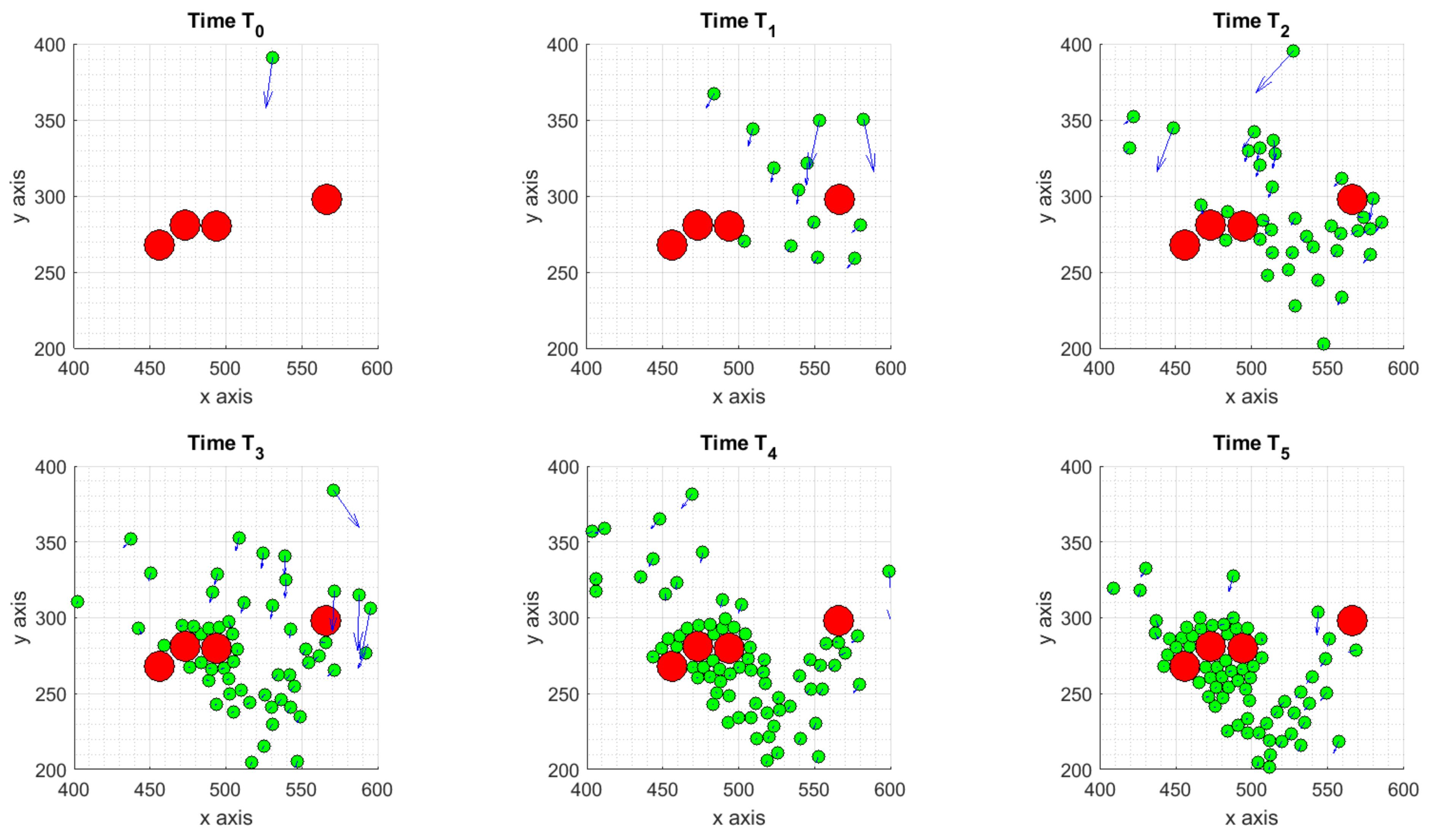
3.1.1. Scenario 1: Deterministic Motion

In Figure 4 we show the final concentration of the chemoattractant, plotted as a 2D surface with a focus on the contour lines (left), and at the boundary of the domain and in correspondence of the centers of the TCs as a function of the longitudinal (center) and transverse distance (right). Cutting the surface this way, the maximum concentrations related to each TC are highlighted.

In Figure 5 the time evolution of the migratory activity of ICs at six different times is depicted. At the initial time, only one IC enters the domain, while at time $T_1$ the number of ICs increases, and they are directed towards the tumor. As the time grows, most of the ICs approach the TCs and stay nearby, accumulating around them; while the others, guided by the inflow of chemical signal, move towards the left-bottom boundaries of the domain.

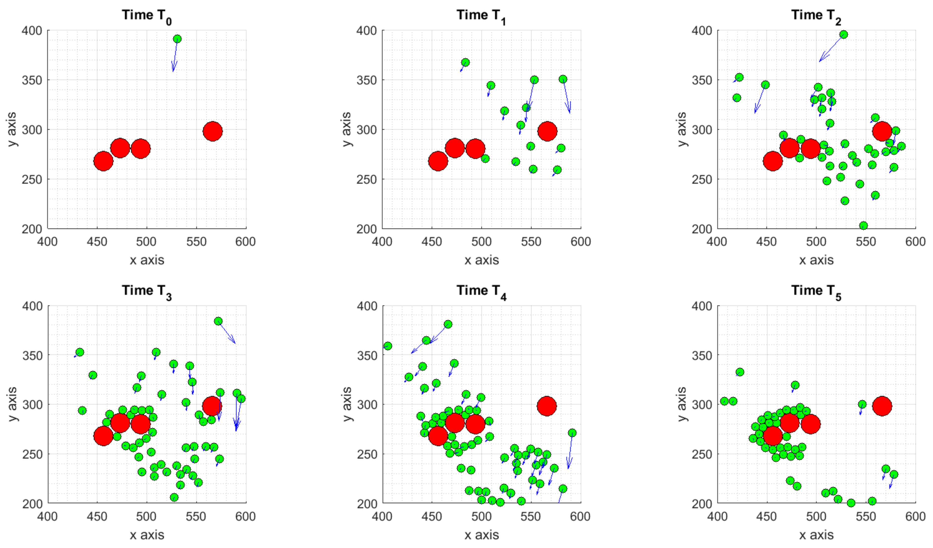
3.1.2. Scenario 2: Deterministic Motion including Cell Death

The biological experiment inspiring our work is related to the phase of immunogenic cell death, during which the TCs, previously treated with a drug, release alarm molecules sensed by the immune system. This latter reacts, attacking the tumor.

In the current scenario we focus on the description of the effects of cell death on the ICs dynamics. We remark that in this preliminary study, we did not insert a specific term in the model to describe the death of TCs due to ICs, but we directly turned off some TCs. Of course, this represents a simplification of what happens in reality, but is here applied for illustrative purposes. However, in the next future we will include in our modeling the death of cancer cells as a consequence of killing activity of ICs, similarly to the modeling proposed in [21].

Please note that in this simplified setting we let dead TCs physically remain in the domain, thus the effects of repulsion with ICs are still effective, but they do not release alarm molecules anymore. This provokes a decrease of the internal concentration due to the absence of previous sources. In the following, we turn off the third TC during the time interval $[T_2,T_3]$, and then we turn off also the fourth TC in the time interval $[T_3,T_4]$. Figure 4 shows the level of the initial concentration (interval $[T_0,T_2]$), while Figure 6 presents the evolution of the concentration after cell death. Comparing Figure 6 with Figure 4, we can observe how the overall concentration decreases after the two cells are killed.

Figure 7 shows the ICs dynamics. At time $T_2$ both the third and the fourth cells are approached by ICs, while at time $T_3$ ICs start moving away from the third cell, which was previously killed and not releasing chemicals anymore. Between time $T_3$ and $T_4$ also the fourth cell is turned off and from time $T_4$ onwards it is not approached anymore. The effect of cell death of some tumor cells (the cells 3 and 4 depicted in Figure 3) on ICs dynamics is depicted in Figure 7. Please note that in the present case a different behavior respect to the one depicted in Figure 5 is observed, since here the accumulation around dead cancer cells does not occur, as expected.

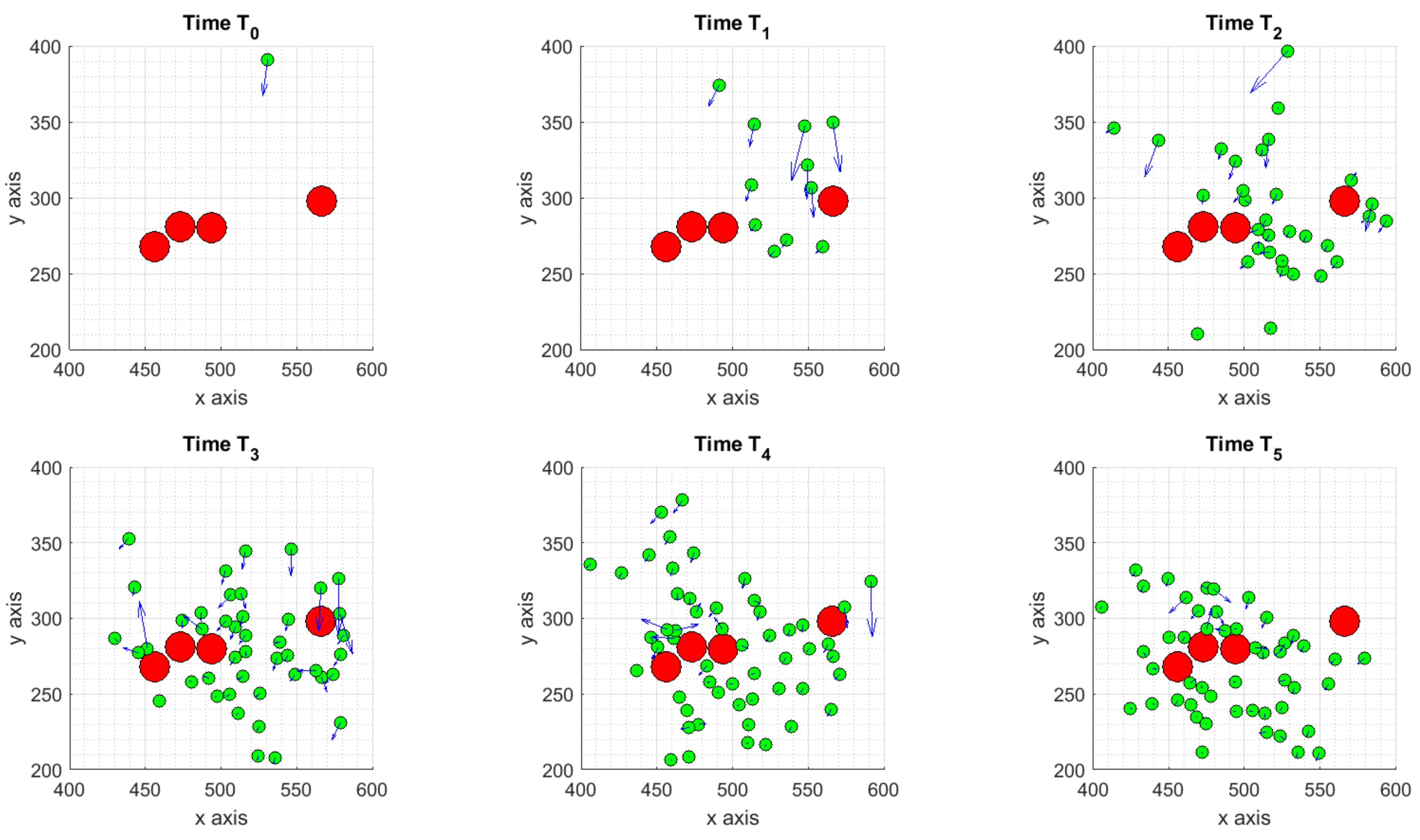
3.1.3. Scenario 3: Stochastic Motion

Several chemical signals are produced at sites of dying TCs and then diffuse into the surrounding environment. ICs sense these chemoattractants and move in the direction where their concentration is greatest, therefore locating the source of the chemoattractants and their associated targets. If on one hand the deterministic model allows us to control the direction of motion of the ICs acting of the concentration of chemicals, on the other hand the complex migratory activity of ICs is better described by a stochastic model, that takes into account the variability of cells, over the preset deterministic mechanisms. For this reason, the features of this last scenario seem to be more suitable to qualitatively describe the real problem.

Estimates of standard deviations. Here we preliminary determine an appropriate value for the standard deviation $\sigma$ in Equation (17). To this end, we consider the trajectory $P_i$ of the i-th IC, for $i=1,\dots ,N_{tot,I}$ and its corresponding smoothing $S_i$, obtained with a moving average (the Matlab © smooth function), and we compute the variance of each IC trajectory:

$${\sigma }_i^2={\displaystyle \frac{1}{T_i}}\sum _{k=1}^{T_i}{(P_i^k-S_i^k)}^2,$$

(18)

where $T_i$ is the number of frames the i-th IC spends on the domain $\Omega$ and we obtain the sequence $\Sigma ={\left\{{\sigma }_i^2\right\}}_{i=1,\dots ,N_{tot,I}}$. Successively, we average the values of $\Sigma$ and divide by $120 \mathrm{s}$, which corresponds to the time interval between two consecutive frames:

$${\sigma }^2=\left({\displaystyle \frac{1}{N_{tot,I}}}\sum _{i=1}^{N_{tot,I}}{\sigma }_i^2\right)/120,$$

(19)

obtaining a variance expressed in seconds. As a last step, we apply the square root to relation (19) and then obtain the standard deviation $\sigma$ of real trajectories. From the analysis conducted on the total number of ICs, we observed cells with variances very far from the average, probably because of the presence of different cell species among the group of ICs. We remark that the immune cell population is heterogeneous, since it is composed by T-lymphocites, monocites, dendritic cells; however, a clear distinction among cell species is not possible currently. For this reason, in order to obtain homogeneous data, we neglect these cell trajectories in the computation of the standard deviation. Indeed, our mathematical model aims at describing an average behavior, and therefore the trajectories whose variance is too far from the average are discarded.

In the presence of more data, we will try to make a classification of cells based on their pathways (length, stops, tortuosity, etc.). This will be the subject of a future study.

The cleaned standard deviations computed from experimental trajectories are reported in Table 1.

ICs dynamics. Figure 8 captures ICs at six different times, while Figure 4 shows the evolution of the chemoattractant. Differences with the deterministic dynamics shown in Figure 5 can be highlighted. In the stochastic case, ICs are more spread.

The computations for this case are performed with a finer time spacing of $\Delta t=10 \mathrm{s}$, with the aim of better describing by the model the complex mechanisms really happening to cells at smaller time scales, and then, the plots are taken every $2\min$, which is the timeframe of video recordings.

As an example, in order to evaluate the effects of the stochastic component on the dynamics and establish a qualitative comparison with the deterministic model, we depict the trajectories of six randomly selected cells. In Figure 9 we assume the starting point of a given experimental cell and show the trajectories obtained with the ODE model (blue) and the SDE model (red), while the corresponding trajectory extracted from the video footage is plotted in black. As can be observed, the deterministic trajectories are smooth and tend, in most cases, to stop in correspondence of the TCs, showing that once the immune cells have fallen in the basin of attraction of the tumor, they tend to be trapped there. The stochastic trajectories, instead, have a more similar behavior to the real ones, showing that after some time spent near the tumor, the immune cells move to the boundary.

So far the Brownian motion yields satisfactory results as shown in Figure 9, but we do not exclude in the next future to deal with more homogeneous and richer dataset to better identify the probability distribution and then apply a general Levý walk.

Table 1. Estimates of physical parameter values.

Parameter	Description	Units	Value	Ref.
$N_{tot,I}$	Number of ICs in $\Omega$ during 24 h		97	Experimental Data
$N_{tot,C}$	Number of TCs in $\Omega$ during 24 h		4	Experimental Data
$L_x$	Horizontal size of $\Omega$	$\mathsf{\mu }\mathrm{m}$	$200$	Experimental Data
$L_y$	Vertical size of $\Omega$	$\mathsf{\mu }\mathrm{m}$	$200$	Experimental Data
$R_I$	IC radius	$\mathsf{\mu }\mathrm{m}$	$4$	[57]
$R_T$	TC radius	$\mathsf{\mu }\mathrm{m}$	$10$	[58,59]
$\overline{R}$	Detection radius of chemicals	$\mathsf{\mu }\mathrm{m}$	$7$	Biological Assumption
$R_3$	Radius of action of repulsion between ICs	$\mathsf{\mu }\mathrm{m}$	$8$	Biological Assumption
$R_4$	Radius of action of adhesion between ICs	$\mathsf{\mu }\mathrm{m}$	$10$	Biological Assumption
$R_1$	Radius of action of Repulsion between ICs and TCs	$\mathsf{\mu }\mathrm{m}$	$14$	Biological Assumption
D	Diffusion Coefficient	$\mathsf{\mu }{\mathrm{m}}^2.{\mathrm{s}}^{-1}$	$2\times {10}^2$	[60]
$\xi$	Growth Rate of f	${\mathrm{s}}^{-1}/\mathrm{cell}$	${10}^{-1}$	[61]
$\eta$	Consumption Rate of f	${\mathrm{s}}^{-1}$	${10}^{-4}$	[61]
${\omega }_{adh}$	Coefficient of Adhesion between ICs	${\mathrm{s}}^{-2}$	${10}^{-7}$	Biological Assumption
${\omega }_{rep}$	Coefficient of Repulsion between ICs	$\mathsf{\mu }{\mathrm{m}}^2.{\mathrm{s}}^{-2}$	$5\times {10}^{-4}$	Biological Assumption
${\omega }_{re{p}_{TI}}$	Coefficient of Repulsion between ICs and TCs	$\mathsf{\mu }{\mathrm{m}}^2.{\mathrm{s}}^{-2}$	$8.5\times {10}^{-3}$	Biological Assumption
$\mu$	Damping Coefficient	${\mathrm{s}}^{-1}$	$2.1\times {10}^{-3}$	Biological Assumption
$k_1$	Cellular Drift Velocity	$\mathrm{mol}.\mathsf{\mu }{\mathrm{m}}^2.{\mathrm{s}}^{-1}$	$0.39$	[60]
$k_2$	Receptor Dissociation Constant	$\mathrm{mol}.\mathsf{\mu }{\mathrm{m}}^{-2}$	$5\times {10}^{-6}$	[60]
a	Rate of exchange of the Chemoattractant with the external environment	$\mathsf{\mu }\mathrm{m}.{\mathrm{s}}^{-1}$	10	Biological Assumption
$\gamma$	Coefficient of Chemotactic Effect. Scenarios 1 and 2	$\mathsf{\mu }{\mathrm{m}}^{-1}$	$5\times {10}^{-3}$	Biological Assumption
$b_1$	Flux condition on $y=0$. Scenarios 1 and 2	$\mathrm{mol}.{\mathrm{s}}^{-1}.\mathsf{\mu }{\mathrm{m}}^{-1}$	$22$	Biological Assumption
$b_2$	Flux condition on $x=L_x$	$\mathrm{mol}.{\mathrm{s}}^{-1}.\mathsf{\mu }{\mathrm{m}}^{-1}$	$12$	Biological Assumption
$b_3$	Flux condition on $y=L_y$	$\mathrm{mol}.{\mathrm{s}}^{-1}.\mathsf{\mu }{\mathrm{m}}^{-1}$	$0$	Biological Assumption
$b_4$	Flux condition on $y=0$. Scenarios 1 and 2	$\mathrm{mol}.{\mathrm{s}}^{-1}.\mathsf{\mu }{\mathrm{m}}^{-1}$	$18$	Biological Assumption
${\sigma }_x$	Standard Deviation of x-trajectories	$\mathsf{\mu }\mathrm{m}.{\mathrm{s}}^{-1/2}.$	$1.49\times {10}^{-1}$	Experimental Data
${\sigma }_y$	Standard Deviation of y-trajectories	$\mathsf{\mu }\mathrm{m}.{\mathrm{s}}^{-1/2}.$	$1.74\times {10}^{-1}$	Experimental Data

Table 1. Estimates of physical parameter values.

Parameter	Description	Units	Value	Ref.
$N_{tot,I}$	Number of ICs in $\Omega$ during 24 h		97	Experimental Data
$N_{tot,C}$	Number of TCs in $\Omega$ during 24 h		4	Experimental Data
$L_x$	Horizontal size of $\Omega$	$\mathsf{\mu }\mathrm{m}$	$200$	Experimental Data
$L_y$	Vertical size of $\Omega$	$\mathsf{\mu }\mathrm{m}$	$200$	Experimental Data
$R_I$	IC radius	$\mathsf{\mu }\mathrm{m}$	$4$	[57]
$R_T$	TC radius	$\mathsf{\mu }\mathrm{m}$	$10$	[58,59]
$\overline{R}$	Detection radius of chemicals	$\mathsf{\mu }\mathrm{m}$	$7$	Biological Assumption
$R_3$	Radius of action of repulsion between ICs	$\mathsf{\mu }\mathrm{m}$	$8$	Biological Assumption
$R_4$	Radius of action of adhesion between ICs	$\mathsf{\mu }\mathrm{m}$	$10$	Biological Assumption
$R_1$	Radius of action of Repulsion between ICs and TCs	$\mathsf{\mu }\mathrm{m}$	$14$	Biological Assumption
D	Diffusion Coefficient	$\mathsf{\mu }{\mathrm{m}}^2.{\mathrm{s}}^{-1}$	$2\times {10}^2$	[60]
$\xi$	Growth Rate of f	${\mathrm{s}}^{-1}/\mathrm{cell}$	${10}^{-1}$	[61]
$\eta$	Consumption Rate of f	${\mathrm{s}}^{-1}$	${10}^{-4}$	[61]
${\omega }_{adh}$	Coefficient of Adhesion between ICs	${\mathrm{s}}^{-2}$	${10}^{-7}$	Biological Assumption
${\omega }_{rep}$	Coefficient of Repulsion between ICs	$\mathsf{\mu }{\mathrm{m}}^2.{\mathrm{s}}^{-2}$	$5\times {10}^{-4}$	Biological Assumption
${\omega }_{re{p}_{TI}}$	Coefficient of Repulsion between ICs and TCs	$\mathsf{\mu }{\mathrm{m}}^2.{\mathrm{s}}^{-2}$	$8.5\times {10}^{-3}$	Biological Assumption
$\mu$	Damping Coefficient	${\mathrm{s}}^{-1}$	$2.1\times {10}^{-3}$	Biological Assumption
$k_1$	Cellular Drift Velocity	$\mathrm{mol}.\mathsf{\mu }{\mathrm{m}}^2.{\mathrm{s}}^{-1}$	$0.39$	[60]
$k_2$	Receptor Dissociation Constant	$\mathrm{mol}.\mathsf{\mu }{\mathrm{m}}^{-2}$	$5\times {10}^{-6}$	[60]
a	Rate of exchange of the Chemoattractant with the external environment	$\mathsf{\mu }\mathrm{m}.{\mathrm{s}}^{-1}$	10	Biological Assumption
$\gamma$	Coefficient of Chemotactic Effect. Scenarios 1 and 2	$\mathsf{\mu }{\mathrm{m}}^{-1}$	$5\times {10}^{-3}$	Biological Assumption
$b_1$	Flux condition on $y=0$. Scenarios 1 and 2	$\mathrm{mol}.{\mathrm{s}}^{-1}.\mathsf{\mu }{\mathrm{m}}^{-1}$	$22$	Biological Assumption
$b_2$	Flux condition on $x=L_x$	$\mathrm{mol}.{\mathrm{s}}^{-1}.\mathsf{\mu }{\mathrm{m}}^{-1}$	$12$	Biological Assumption
$b_3$	Flux condition on $y=L_y$	$\mathrm{mol}.{\mathrm{s}}^{-1}.\mathsf{\mu }{\mathrm{m}}^{-1}$	$0$	Biological Assumption
$b_4$	Flux condition on $y=0$. Scenarios 1 and 2	$\mathrm{mol}.{\mathrm{s}}^{-1}.\mathsf{\mu }{\mathrm{m}}^{-1}$	$18$	Biological Assumption
${\sigma }_x$	Standard Deviation of x-trajectories	$\mathsf{\mu }\mathrm{m}.{\mathrm{s}}^{-1/2}.$	$1.49\times {10}^{-1}$	Experimental Data
${\sigma }_y$	Standard Deviation of y-trajectories	$\mathsf{\mu }\mathrm{m}.{\mathrm{s}}^{-1/2}.$	$1.74\times {10}^{-1}$	Experimental Data

4. Parameters Estimation on Synthetic Data

In this Section we present the calibration algorithm for the estimation of some model parameters and the results obtained with it. All the model parameters are reported in Table 1. We underline that some of them are given from experimentalists since are taken from the laboratory experiment (size of the cropped area, number of TCs and ICs across time, standard deviation of cell pathways). Other parameters, such as for instance, the diffusion coefficient of chemoattractant, cellular drift velocity, receptor dissociation constant or the radii of cells are taken from the literature. For the model parameters whose values still need to be assigned, we assumed fixed most of them, such as the radii of action between cells or adhesion/repulsion coefficients among cells, setting them in a phenomenological way through the observation of their effects on the overall dynamics.

Then, in order to reduce the computational cost of the optimization procedure, we apply our calibration procedure only to 4 model parameters, i.e., the coefficient of chemotactic effect $\gamma$, and the chemical inflow, respectively, at the left, right and bottom boundaries $b_1,b_2,b_4$, since we observed qualitatively a great effect of such parameters on the overall dynamics and, as a simplification of the model, we assume $b_3=0$. In particular, the coefficient $\gamma$ affects the speed of ICs, while $b_1,b_2,b_4$ affect the directionality of immune cells.

We underline that the parameter estimation procedure here described is applied to the deterministic version of the model, i.e., (3) and (4). An extension of this procedure to calibrate the stochastic model (3)–(17) will be included in a future work.

In this methodological study we want to show the feasibility and applicability of such estimation technique for some significant model parameters of the hybrid model describing Cancer-on-Chip experiment. Our final goal is indeed not the exact fitting of model parameters, but is to show that we are able to qualitatively reproduce the dynamics observed experimentally, even if the quantification of the chemical gradients in the environment is currently impossible for biologists in this kind of experiments. In the next future, we will complement this methodology with macroscopic models deriving from them to be able to simulate immunocompetent behavior in organs and tissues, where millions of cells are present. To this aim, we applied the proposed procedure to a synthetic dataset produced by the model itself—but strongly inspired by experimental one—to assess the soundness of this strategy. In the future, we aim at having more data in such a way to apply the proposed strategy to a real biological dataset.

Data preparation.

To succeed in the calibration of model parameters, we need to extract a common behavior from the time-varying trajectories of immune cells located at different points of the observed area. Thus, here we propose a calibration algorithm taking into account this variability constructing a “realistic” synthetic dataset of ICs pathways that can reproduce qualitatively the real trajectories extracted from the video footage of the experiment. In particular, a set of trajectories of cells sharing an average behavior has been produced by suitably tuning model parameters to have an upper and lower bound of cell speeds taken from the experimentally observed ones. Then, ICs velocity field given by 2D surface is computed by the model itself at every observation time of 2 min (as the video footage timeframe). It is worth noting that the application of this strategy implies the assumption to have a single population of immune cells showing an average behavior.

The velocity field is then approximated using a multidimensional spline interpolation technique, described in Section 4.1 to have smoothing in time and space on the dataset to be compared.

Main steps of the calibration algorithm.

The calibration algorithm applied to estimate crucial model parameters can be summarized as follows:

• the dataset representing the target solutions of our procedure computed from synthetic ICs trajectories is obtained by the model with fixed parameters;
• a time-space approximation of the velocity fields is carried out with the spline technique presented in Section 4.1 and used as target solution of the calibration algorithm;
• perturbed model parameters are used as initial guess of a global search algorithm minimizing the norm of the difference between the target velocity fields and the estimated ones, as explained in Section 4.2.

The results obtained with the procedure above are reported in Section 4.3.

4.1. Multidimensional Interpolation

The position and speed of the ICs, variable in time, provide punctual information about the velocity field in which the ICs are immersed. As a consequence, they can be considered to be training points for the calibration of an interpolation algorithm, able to provide information about the full space. Here we are considering time as the third dimension, being x and y the first two. As the interpolation scheme we are using a multidimensional spline, described in [31].

Each training point is supposed to influence the value of the interpolating function over a (limited) portion of the space in proximity of it. The degree of influence of the ith training point ($w_i(x,y,t)$) is a function of time and space, driven by a compact-support function radial basis decaying at zero outside the influence area. Then, the interpolated value is obtained as a weighted sum of the values at the training points:

$$\tilde{v}(x,y,t)=\sum _{i=1}^n{w}_i(x,y,t)h\left(i\right)c\left(i\right),$$

(20)

where $c\left(i\right)$ represents the value of the interpolating function at the ith training point and n is the total data-points available, corresponding to $t_1,\dots ,t_n$ discrete times. Specifically, we have two functions $\tilde{v}$, i.e., ${\tilde{v}}_x(x,y,t)$ and ${\tilde{v}}_y(x,y,t)$. Moreover, the vector $c\left(i\right)$ is different according to the velocities under exam, with training points corresponding alternatively to the x- and y-velocities. Since different influence areas may overlap, the value of $w_i(x,y,t)$ needs to be adjusted to have a correct fit. To this aim, we need to solve a linear system where the n Equations (20) are collocated at the training points, generating an $n\times n$ system. The n coefficients $h\left(i\right)$ are computed only once, and then applied in the interpolation procedure. In this specific case, we are using a linear function for the influence coefficients $w_i(x,y,t)$.

4.2. The Calibration Algorithm

With Formula (20) we have generated a velocity field $\tilde{v}$ that from now on we indicate as $V^e$ to point out that the velocity field is produced with the punctual velocities v the immune cells assume at every time step, coming from experimental data (in this specific case from synthetic data). Later we have used this field to define an appropriate functional to be minimized.

To assess the goodness and soundness of our strategy, the analysis which follows is performed on synthetic data, i.e., numerical data produced by the PDE–ODEs system (3) and (4). Future work will be directed towards the application of this methodology to the experimental outcomes.

As a first step we have interpolated immune cell velocities v obtained from synthetic data to the end of generating a velocity field to use as a target, in correspondence of every frame. Thus, we have produced $T_f=681$ velocity fields $V_x^e$ using the punctual velocities in x and $T_f=681$ velocity fields $V_y^e$ using the velocities in y. In Figure 10 we present an example of the surfaces resulting from the interpolation at a certain time step. Figure 10A shows the interpolation of the x-velocities, while Figure 10B shows the interpolation of the y-velocities. The green points have coordinates $(P_x,P_y,v_x)$ in (A) and $(P_x,P_y,v_y)$ in (B). For more details about the interpolation technique see Section 4.1.

Successively, we have launched the optimization algorithm and at every run we have computed the numerical solutions of the deterministic model with the approximation scheme described in Appendix A. We have then built a routine in which inserting the numerical positions we are able to find the corresponding velocities on the surface $V^e$. The resulting interpolated velocities $V^n$ are then used to construct the objective function:

$$J_V\left(\theta \right)={\left[{\displaystyle \frac{1}{T_f}}\sum _{k=1}^{T_f}\left({\displaystyle \frac{1}{N_{tot,I}^k}}\sum _{i=1}^{N_{tot,I}^k}{\displaystyle \frac{\left|\right|V_i^{e,k}-V_i^{n,k}\left(\theta \right)\left|\right|}{\left|\right|V_i^{e,k}\left|\right|}}\right)\right]}^2.$$

(21)

In (21) we compare at every time step the punctual interpolated velocities with the punctual target velocities, i.e., the velocities used to generate the field. With $\theta$ we indicate the vector whose dimension corresponds to the parameter values we search.

In addition, we have also included a Tikhonov regularization term in the functional, as usually done for the regularization of linear inverse problems. In particular, we consider the following term to be added to the functional to be minimized:

$$P_{\lambda }\left(\theta \right)={\lambda }^2\left|\right|\theta -{\theta }_0{\left|\right|}^2,$$

(22)

where ${\theta }_0$ are the a priori estimate of target parameter values and $\theta$ are the parameter values we are optimizing. The constant $\lambda$ is a regularization parameter that helps the algorithm in the search for optimal values of model parameters by reducing the number of local minima in the functional, see [62]. Tests for different values of $\lambda$ showed better results of the calibration algorithm for ${\lambda }^2=0.1$. Thus, with relation (22) we want to reduce the error between the target values and the searched ones.

With functionals (21) and (22) we can define the minimization problem:

$$\underset{\theta \in \Theta }{min}J\left(\theta \right)=\underset{\theta \in \Theta }{min}(J_V\left(\theta \right)+P_{\lambda }\left(\theta \right)),$$

(23)

where $\Theta$ is the space to explore to search the unknown parameter values. For completeness, we introduce another estimator we have used for our simulations, which is based on the idea of comparing the distances assumed by the tumor and immune cells at every time step. We indicate with $C_j$ the position of the j-th TC (the temporal indicator k is omitted since TC positions do not evolve in time). We call $d_{i,j}^k$ the distance between the i-th IC and the j-th TC at time k:

$$d_{i,j}^k=\left|\right|P_i^k-C_j\left|\right|,$$

(24)

and then, fixed the i-th IC, we compare the distances $d_{i,j}^{n,k}$ obtained from the numerical positions with the distances $d_{i,j}^{e,k}$ obtained from the synthetic positions:

$$D_i^k={\displaystyle \frac{1}{N_{tot,c}}}\sum _{j=1}^{N_{tot,c}}{\displaystyle \frac{\left|\right|d_{i,j}^{e,k}-d_{i,j}^{n,k}\left|\right|}{\left|\right|d_{i,j}^{e,k}\left|\right|}},$$

successively, we sum over all ICs:

$$D^k={\displaystyle \frac{1}{N_{tot,i}^k}}\sum _{i=1}^{N_{tot,i}^k}{D}_i^k,$$

and then we sum over all times. To summarize, we have the functional:

$$J_{D_{TI}}={\left[{\displaystyle \frac{1}{T_f}}\sum _{k=1}^{T_f}\left({\displaystyle \frac{1}{N_{tot,i}^k}}\sum _{j=1}^{N_{tot,i}}\left({\displaystyle \frac{1}{N_{tot,c}}}\sum _{j=1}^{N_{tot,c}}{\displaystyle \frac{\left|\right|d_{i,j}^{e,k}-d_{i,j}^{n,k}\left|\right|}{\left|\right|d_{i,j}^{e,k}\left|\right|}}\right)\right)\right]}^2.$$

(25)

In conclusion, to evaluate the error committed by the optimization with respect to synthetic data, we indicate with ${\theta }_0$ the target value and with ${\theta }^{*}$ the corresponding optimized parameter and we define:

$$RE={\displaystyle \frac{\left|\right|{\theta }^{*}-{\theta }_0\left|\right|}{\left|\right|{\theta }^{*}\left|\right|}}\times 100,$$

(26)

the approximation error of each parameter.

The minimization of the functionals above is performed with Particle Swarm Optimization (PSO) [63] as search method using the Matlab ©toolbox. For the approximation of target and computed velocity fields resulting in a 2D varying in time surface we use a spline multidimensional interpolation described in Section 4.1.

4.3. Results on Parameters Estimation

Tests on the calibration algorithm are performed to assess the goodness and robustness of the methodology shown in Section 4.2. Please note that the total number of parameters to be assigned is 14, since the other parameters are given from the experimentalists or taken from the literature, as reported in Table 1. Of course, it is possible to make a parameter estimation of all of them. However, in the present work, in order to reduce the computational cost, we apply our calibration procedure only to 4 model parameters that we consider very significant since they strongly affect the dynamics of the ICs, i.e., $\gamma ,b_1,b_2$ and $b_4$.

We recall the $\gamma$ is the coefficient which enhances the effect of the chemotactic function (5), while $b_i$, for $i=1,2,4$ are the parameters that control the chemical inflow at the boundaries. In order to perform the tests, we produced synthetic solutions choosing specific values for the listed parameters:

$$\gamma =5·{10}^{-3},b_1=22,b_2=12,b_4=18,$$

(27)

which correspond to those used to create the Scenario 1 (see Section 3.1.1). The synthetic solutions are used to generate the velocity fields $V^e$ to be used as targets.

To assess our strategy, we start testing one parameter and then adding one more at time. The range for the parameter variations is chosen by varying the initial guess by a percentage of $\pm 50\%$. Specifically, we searched $\gamma$ in $I_{50\%}=[3.5\mathrm{e}-3,6.5\mathrm{e}-3]$, $b_1$ in $I_{50\%}=[11,33]$, $b_2$ in $I_{50\%}=[6,18]$ and $b_4$ in $I_{50\%}=[9,27]$. We also choose as initial guess a perturbation of the model parameters by $+30\%$. We tested the algorithm with the following two different functionals:

$$J_1=J_V+P_{\lambda },$$

(28)

and

$$J_2=J_V+J_{D_{TI}}+P_{\lambda }.$$

(29)

Results with the functional $J_1$ are reported in

Table 2. $J_1$. Deterministic Model Calibration. Parameter $\gamma =5\times {10}^{-3}$, parameter $b_1=22$, parameter $b_4=18$ and parameter $b_2=12$ are varied by $+30\%$ and they are optimized in the range $\pm 50\%$.

Functional	RE %	RE %	RE %	RE %	${\mathit{J}}_{\mathit{V}}$	${\mathit{P}}_{\mathit{\lambda }}$	Fval
	$\mathbf{\gamma }$	${\mathit{b}}_{\mathbf{1}}$	${\mathit{b}}_{\mathbf{4}}$	${\mathit{b}}_{\mathbf{2}}$
$J_1$	$4.114\times {10}^{-4}$	-	-	-	$2.076\times {10}^{-7}$	$4.231\times {10}^{-17}$	$2.076\times {10}^{-7}$
	$2.066\times {10}^{-4}$	$5.249\times {10}^{-4}$	-	-	$2.064\times {10}^{-7}$	$1.334\times {10}^{-9}$	$2.078\times {10}^{-7}$
	$7.874\times {10}^{-5}$	$2.397\times {10}^{-4}$	$2.283\times {10}^{-4}$	-	$2.064\times {10}^{-7}$	$2.633\times {10}^{-10}$	$2.067\times {10}^{-7}$
	$1.353\times {10}^{-3}$	$1.869\times {10}^{-3}$	$5.18\times {10}^{-4}$	$7.41\times {10}^{-4}$	$2.09\times {10}^{-7}$	$1.857\times {10}^{-8}$	$2.275\times {10}^{-7}$

, while results with $J_2$ are in

Table 3. $J_2$. Deterministic Model Calibration. Parameter $\gamma =5\times {10}^{-3}$, parameter $b_1=22$, parameter $b_4=18$ and parameter $b_2=12$ are varied by $+30\%$ and they are optimized in the range $\pm 50\%$.

Functional	RE %	RE %	RE %	RE %	${\mathit{J}}_{\mathit{V}}$	${\mathit{P}}_{\mathit{\lambda }}$	Fval
	$\mathbf{\gamma }$	${\mathit{b}}_{\mathbf{1}}$	${\mathit{b}}_{\mathbf{4}}$	${\mathit{b}}_{\mathbf{2}}$
$J_2$	$2.915\times {10}^{-6}$	-	-	-	$2.064\times {10}^{-7}$	$2.833\times {10}^{-14}$	$2.134\times {10}^{-21}$	$2.064\times {10}^{-7}$
	$2.798\times {10}^{-5}$	$4.558\times {10}^{-4}$	-	-	$2.068\times {10}^{-7}$	$2.037\times {10}^{-8}$	$1.006\times {10}^{-9}$	$2.281\times {10}^{-7}$
	$2.93\times {10}^{-4}$	$4.335\times {10}^{-4}$	$7.67\times {10}^{-4}$	-	$2.066\times {10}^{-7}$	$6.273\times {10}^{-10}$	$2.816\times {10}^{-9}$	$2.1\times {10}^{-7}$
	$1.102\times {10}^{-4}$	$5.503\times {10}^{-4}$	$1.63\times {10}^{-4}$	$2.65\times {10}^{-4}$	$2.064\times {10}^{-7}$	$4.662\times {10}^{-10}$	$1.653\times {10}^{-9}$	$2.085\times {10}^{-7}$

. In each row of Table 2 and Table 3 errors obtained with the parameter estimation algorithm are reported. Please note that errors are reported in increasing order respect to the number of parameters involved in the parameter estimation procedure, from the top to the bottom. We can notice that in both cases the errors in parameters estimation are quite low since their order of magnitude is around ${10}^{-3}$ in the worst case, meaning the calibration was successful. We also underline that the norm of the total error of the functional is low, around ${10}^{-7}$, given by the $J_V$ component.

In conclusion, as a way to quantify the goodness of our reconstruction, we compute the percentage of cells passing through the cropped area of the chip representing the computational domain. In particular, we depict with histograms the statistics obtained from the trajectories reconstructed by the calibrated model and the statistics computed from the trajectories of the synthetic dataset, i.e., the target solutions of the calibration algorithm. The percentage of outgoing cells $N_o^k$ over the number of cells $N_p^k$ present in the domain $\Omega$, is computed by the formula:

$$N^k={\displaystyle \frac{N_o^k}{N_p^k}}\times 100,$$

(30)

for each timeframe $k=1,\dots ,680$ with a time spacing of 2 min. Then, the optimized parameters (27) obtained with the calibration procedure described in Section 4.2 are used as the model parameters to be given in input to both the ODE model (3) and (4) and the SDE model (3)–(17) for the computation of the statistics on cell trajectories. More precisely, we perform this computation for the target case, i.e., the synthetic trajectories obtained by the PDE–ODEs system (yellow bars in Figure 11). Then, assuming randomly placed initial positions of ICs, we compute the same statistics for the PDE–ODEs system (red bars in Figure 11) and for the PDE-SDEs system (blue bars in Figure 11). In particular, the initial positions $P_i^k$, for $i=1,\dots ,N_{tot,I}$ are randomly perturbed in a range of (0, 5] $\mathsf{\mu }$m. As can be seen in Figure 11, the statistics of target trajectories (ODE-target) and reconstructed trajectories (ODE-modified and SDE-modified) are quite similar in terms order of magnitude. Please note that the ODE-modified shows the ability to reproduce well also the timing of the exits from the domain, while a slight variability, as expected, can be observed in the SDE-modified case in terms of time occurrence of exits from the domain.

5. Conclusions and Future Work

In the present work we have developed a mathematical model to describe the interactions between ICs and treated TCs in microfluidic chip, together with a strategy to estimate unknown parameter values.

Regarding the modeling part, we have introduced a hybrid model, composed of a reaction-diffusion equation to describe the evolution of chemicals released by TCs, coupled with an equation for the motion of each IC, driven by the chemical gradient. The deterministic system represents a first microscopic model of ICs dynamics in a subarea of the chip.

First, we qualitatively analyzed the overall dynamics of ICs, varying important parameters of the system, such as the chemotactic coefficient $\gamma$ and the boundary parameters. Indeed, according to their magnitude, the direction of the motion can be controlled and decided a priori. Then, in order to reproduce some interesting features characterizing cell behavior, we adjusted suitably the model parameters and we presented three different scenarios that can occur in the chip:

• the deterministic scenario, with some ICs attracted by the tumor and others moving towards to the boundaries of the considered domain;
• the cell death scenario, as a subcase of the previous one, obtained assuming two TCs have died after their interaction with ICs, causing changes in the internal concentration of chemicals thus affecting ICs dynamics;
• the stochastic scenario, obtained adding to the equation of the motion a Brownian walk to mimic the randomness on ICs trajectories.

Regarding the stochastic scenario, it is important to highlight that the Brownian motion is not the most appropriate to describe ICs movement, but in the future we aim at substituting it by the Lévy walk. In recent works [64,65], it has indeed emerged that a heavy-tailed process is more efficient and realistic than Brownian motion. However, in the present work, the shortage of data at our disposal did not provide us information on the nature of the different ICs involved in the experiment. To this end, we are working on a classification strategy in a forthcoming paper to be able to identify the different categories of ICs and then differentiate the model parameters according to the corresponding cell type.

In addition to the pure modeling part, we have developed a model calibration procedure based on the comparison of the velocity fields related to ICs at every time step.

The calibration procedure with synthetic data revealed to be successful, thus representing a first step towards the model calibration on experimental data.

Finally, the main achievements of the present work are represented by:

• the development of a simulation algorithm mimicking short-range dynamics of ICs in the neighborhood of TCs, as observed in Cancer-on-Chip experiment;
• the introduction of an ad-hoc methodology for the calibration of model parameters based on the time-space approximation of synthetic velocity fields computed from immune cell trajectories.

Future perspectives.

Our future aim is to extend this framework to validate our model against the experimental velocity fields computed from the real IC trajectories extracted from the video footage of the experiment.

To face the problem of calibrating the model parameters against real data, we first must produce an interpolation model able to take into account the non-deterministic nature of the cell motions. A possible strategy is to produce a stochastic interpolator, able to determine the expected value and variance of the local speed: the final interpolated value will be then obtained adding a stochastic part, computed using the interpolated variance and the same probability density function of the experimental data, to the interpolated expected value. Using this approach, we have a non-deterministic interpolated value with the same statistical qualities of the interpolating dataset. Implicitly, we are considering as deterministic the local values of the expected value and of the variance of our experimental dataset, and we are also assuming to be able to compute the statistical distribution of the real data (otherwise, we can adopt a prescribed distribution. i.e., Gaussian). It is now evident that the comparison cannot be produced on a single path, but we need to observe the trajectories from a statistical standpoint, i.e., comparing the average path over many simulations, whose output is now non-deterministic. At the same time, in order to derive the statistical properties of the real IC trajectories and speed, a large number of experiments is needed, with a time resolution of the same order of magnitude of the time scale of the physical phenomenon under investigation. This implies a huge experimental and numerical effort, one or two order of magnitude larger than the present work.

References

1. Businaro, L.; de Ninno, A.; Schiavoni, G.; Lucarini, V.; Ciasca, G.; Gerardino, A.; Belardelli, F.; Gabriele, L.; Mattei, F. Cross talk between cancer and immune cells: Exploring complex dynamics in a microfluidic environment. Lab Chip 2013, 13, 229–239. [Google Scholar] [CrossRef]
2. Gori, M.; Simonelli, M.C.; Giannitelli, S.M.; Businaro, L.; Trombetta, M.; Rainer, A. Investigating Nonalcoholic Fatty Liver Disease in a Liver-on-a-Chip Microfluidic Device. PLoS ONE 2016, 11, e0159729. [Google Scholar] [CrossRef] [PubMed]
3. Huh, D.; Matthews, B.D.; Mammoto, A.; Montoya-Zavala, M.; Hsin, H.Y.; Ingber, D.E. Reconstituting Organ-Level Lung Functions on a Chip. Science 2010, 328, 1662–1668. [Google Scholar] [CrossRef] [PubMed] [Green Version]
4. Graney, P.L.; Tavakol, D.N.; Chramiec, A.; Ronaldson-Bouchard, K.; Vunjak-Novakovic, G. Engineered models of tumor metastasis with immune cell contributions. iScience 2021, 24, 102179. [Google Scholar] [CrossRef]
5. Mattei, F.; Andreone, S.; Mencattini, A.; De Ninno, A.; Businaro, L.; Martinelli, E.; Schiavoni, G. Oncoimmunology Meets Organs-on-Chip. Front. Mol. Biosci. 2021, 8, 627454. [Google Scholar] [CrossRef]
6. Maulana, T.I.; Kromidas, E.; Wallstabe, L.; Cipriano, M.; Alb, M.; Zaupa, C.; Hudecek, M.; Fogal, B.; Loskill, P. Immunocompetent cancer-on-chip models to assess immuno-oncology therapy. Adv. Drug Deliv. Rev. 2021, 173, 281–305. [Google Scholar] [CrossRef] [PubMed]
7. Vacchelli, E.; Ma, Y.; Baracco, E.E.; Sistigu, A.; Enot, D.P.; Pietrocola, F.; Yang, H.; Adjemian, S.; Chaba, K.; Semeraro, M.; et al. Chemotherapy-induced antitumor immunity requires formyl peptide receptor 1. Science 2015, 350, 972–978. [Google Scholar] [CrossRef]
8. Parlato, S.; Grisanti, G.; Sinibaldi, G.; Peruzzi, G.; Casciola, C.M.; Gabriele, L. Tumor-on-a-chip platforms to study cancer–immune system crosstalk in the era of immunotherapy. Lab Chip 2020, 21, 234–253. [Google Scholar] [CrossRef]
9. Montanez-Sauri, S.I.; Sung, K.E.; Berthier, E.; Beebe, D.J. Enabling screening in 3D microenvironments: Probing matrix and stromal effects on the morphology and proliferation of T47D breast carcinoma cells. Integr. Biol. 2013, 5, 631–640. [Google Scholar] [CrossRef] [Green Version]
10. Hassell, B.; Goyal, G.; Lee, E.; Sontheimer-Phelps, A.; Levy, O.; Chen, C.; Ingber, D.E. Human Organ Chip Models Recapitulate Orthotopic Lung Cancer Growth, Therapeutic Responses, and Tumor Dormancy In Vitro. Cell Rep. 2017, 21, 508–516. [Google Scholar] [CrossRef] [Green Version]
11. Baker, B.; Trappmann, B.; Stapleton, S.C.; Toro, E.; Chen, C. Microfluidics embedded within extracellular matrix to define vascular architectures and pattern diffusive gradients. Lab Chip 2013, 13, 3246–3252. [Google Scholar] [CrossRef] [Green Version]
12. Bischel, L.L.; Young, E.W.; Mader, B.R.; Beebe, D.J. Tubeless microfluidic angiogenesis assay with three-dimensional endothelial-lined microvessels. Biomaterials 2012, 34, 1471–1477. [Google Scholar] [CrossRef] [Green Version]
13. Chen, M.B.; Whisler, J.A.; Jeon, J.; Kamm, R.D. Mechanisms of tumor cell extravasation in an in vitro microvascular network platform. Integr. Biol. 2013, 5, 1262–1271. [Google Scholar] [CrossRef] [Green Version]
14. Moya, M.L.; Hsu, Y.-H.; Lee, A.; Hughes, C.C.; George, S.C. In Vitro Perfused Human Capillary Networks. Tissue Eng. Part C Methods 2013, 19, 730–737. [Google Scholar] [CrossRef] [Green Version]
15. Nguyen, D.-H.T.; Stapleton, S.C.; Yang, M.T.; Cha, S.S.; Choi, C.K.; Galie, P.; Chen, C.S. Biomimetic model to reconstitute angiogenic sprouting morphogenesis in vitro. Proc. Natl. Acad. Sci. USA 2013, 110, 6712–6717. [Google Scholar] [CrossRef] [PubMed] [Green Version]
16. Wang, X.; Phan, D.T.T.; Sobrino, A.; George, S.C.; Hughes, C.C.W.; Lee, A.P. Engineering anastomosis between living capillary networks and endothelial cell-lined microfluidic channels. Lab Chip 2015, 16, 282–290. [Google Scholar] [CrossRef]
17. Jeong, S.-Y.; Lee, J.-H.; Shin, Y.; Chung, S.; Kuh, H.-J. Co-Culture of Tumor Spheroids and Fibroblasts in a Collagen Matrix-Incorporated Microfluidic Chip Mimics Reciprocal Activation in Solid Tumor Microenvironment. PLoS ONE 2016, 11, e0159013. [Google Scholar] [CrossRef] [PubMed] [Green Version]
18. Lee, J.-H.; Kim, S.-K.; Khawar, I.A.; Jeong, S.-Y.; Chung, S.; Kuh, H.-J. Microfluidic co-culture of pancreatic tumor spheroids with stellate cells as a novel 3D model for investigation of stroma-mediated cell motility and drug resistance. J. Exp. Clin. Cancer Res. 2018, 37, 1–12. [Google Scholar] [CrossRef] [PubMed] [Green Version]
19. Ramaswamy, S.; Ross, K.N.; Lander, E.S.; Golub, T.R. A molecular signature of metastasis in primary solid tumors. Nat. Genet. 2002, 33, 49–54. [Google Scholar] [CrossRef] [PubMed]
20. Zervantonakis, I.; Hughes, S.; Charest, J.L.; Condeelis, J.S.; Gertler, F.B.; Kamm, R.D. Three-dimensional microfluidic model for tumor cell intravasation and endothelial barrier function. Proc. Natl. Acad. Sci. USA 2012, 109, 13515–13520. [Google Scholar] [CrossRef] [Green Version]
21. Braun, E.; Bretti, G.; Natalini, R. Mass-Preserving Approximation of a Chemotaxis Multi-Domain Transmission Model for Microfluidic Chips. Mathematics 2021, 9, 688. [Google Scholar] [CrossRef]
22. Natalini, R.; Paul, T. On the Mean Field limit for Cucker-Smale models. Discret. Contin. Dyn.-Syst. B 2021. [Google Scholar] [CrossRef]
23. Agliari, E.; Biselli, E.; De Ninno, A.; Schiavoni, G.; Gabriele, L.; Gerardino, A.; Mattei, F.; Barra, A.; Businaro, L. Cancer-driven dynamics of immune cells in a microfluidic environment. Sci. Rep. 2014, 4, 6639. [Google Scholar] [CrossRef] [PubMed]
24. Zhong, R.X.; Fu, K.Y.; Sumalee, A.; Ngoduy, D.; Lam, W.H. A cross-entropy method and probabilistic sensitivity analysis framework for calibrating microscopic traffic models. Transp. Res. Part C Emerg. Technol. 2016, 63, 147–169. [Google Scholar] [CrossRef]
25. Kirschner, D.; Panetta, J.C. Modeling immunotherapy of the tumor-immune interaction. J. Math. Biol. 1998, 37, 235–252. [Google Scholar] [CrossRef] [PubMed] [Green Version]
26. Lee, S.W.L.; Seager, R.J.; Litvak, F.; Spill, F.; Sieow, J.L.; Leong, P.H.; Kumar, D.; Tan, A.S.M.; Wong, S.C.; Adriani, G.; et al. Integrated in silico and 3D in vitro model of macrophage migration in response to physical and chemical factors in the tumor microenvironment. Integr. Biol. 2020, 12, 90–108. [Google Scholar] [CrossRef]
27. Yang, T.D.; Park, J.-S.; Choi, Y.; Choi, W.; Ko, T.-W.; Lee, K.J. Zigzag Turning Preference of Freely Crawling Cells. PLoS ONE 2011, 6, e20255. [Google Scholar] [CrossRef] [Green Version]
28. Checcoli, A.; Pol, J.G.; Naldi, A.; Noel, V.; Barillot, E.; Kroemer, G.; Thieffry, D.; Calzone, L.; Stoll, G. Dynamical Boolean Modeling of Immunogenic Cell Death. Front. Physiol. 2020, 11, 1320. [Google Scholar] [CrossRef]
29. Braun, E.C. Organs-On-Chips: Mathematical Modelling and Parameter Estimation. Ph.D. Thesis, Universitá degli Studi di Roma Tre, Roma, Italy, 2021. [Google Scholar]
30. Di Costanzo, E.; Natalini, R.; Preziosi, L. A hybrid mathematical model for self-organizing cell migration in the zebrafish lateral line. J. Math. Biol. 2014, 71, 171–214. [Google Scholar] [CrossRef] [Green Version]
31. Peri, D. Easy-to-implement multidimensional spline interpolation with application to ship design optimisation. Ship Technol. Res. 2017, 65, 32–46. [Google Scholar] [CrossRef]
32. Stevens, A.; Othmer, H.G. Aggregation, Blowup, and Collapse: The ABC’s of Taxis in Reinforced Random Walks. SIAM J. Appl. Math. 1997, 57, 1044–1081. [Google Scholar] [CrossRef]
33. Pomeau, Y.; Piasecki, J. The Langevin equation. C. R. Phys. 2017, 18, 570–582. [Google Scholar] [CrossRef]
34. Bai, J.; Tu, T.-Y.; Kim, C.; Thiery, J.P.; Kamm, R.D. Identification of drugs as single agents or in combination to prevent carcinoma dissemination in a microfluidic 3D environment. Oncotarget 2015, 6, 36603–36614. [Google Scholar] [CrossRef] [PubMed] [Green Version]
35. Xu, Z.; Gao, Y.; Hao, Y.; Li, E.; Wang, Y.; Zhang, J.; Wang, W.; Gao, Z.; Wang, Q. Application of a microfluidic chip-based 3D co-culture to test drug sensitivity for individualized treatment of lung cancer. Biomaterials 2013, 34, 4109–4117. [Google Scholar] [CrossRef] [PubMed]
36. De Ninno, A.; Bertani, F.R.; Gerardino, A.; Schiavoni, G.; Musella, M.; Galassi, C.; Mattei, F.; Sistigu, A.; Businaro, L. Microfluidic Co-Culture Models for Dissecting the Immune Response in in vitro Tumor Microenvironments. J. Vis. Exp. 2021, 170, e61895. [Google Scholar] [CrossRef]
37. Kroemer, G.; Galluzzi, L.; Kepp, O.; Zitvogel, L. Immunogenic Cell Death in Cancer Therapy. Annu. Rev. Immunol. 2013, 31, 51–72. [Google Scholar] [CrossRef]
38. Greenberg, J.M.; Alt, W. Stability results for a diffusion equation with functional drift approximating a chemotaxis model. Trans. Am. Math. Soc. 1987, 300, 235. [Google Scholar] [CrossRef]
39. Keller, E.F.; Segel, L.A. Initiation of slime mold aggregation viewed as an instability. J. Theor. Biol. 1970, 26, 399–415. [Google Scholar] [CrossRef]
40. Péré, M.; Chaves, M.; Roux, J. Core Models of Receptor Reactions to Evaluate Basic Pathway Designs Enabling Heterogeneous Commitments to Apoptosis. In Proceedings of the International Conference on Computational Methods in Systems Biology, Konstanz, Germany, 23–25 September 2020; pp. 298–320. [Google Scholar] [CrossRef]
41. Edalgo, Y.T.N.; Zornes, A.L.; Versypt, A.N.F. A hybrid discrete–continuous model of metastatic cancer cell migration through a remodeling extracellular matrix. AIChE J. 2019, 65, e16671. [Google Scholar] [CrossRef]
42. Othmer, H.G.; Kim, Y. Hybrid models of cell and tissue dynamics in tumor growth. Math. Biosci. Eng. 2015, 12, 1141–1156. [Google Scholar] [CrossRef]
43. Perfahl, H.; Hughes, B.; Alarcon, T.; Maini, P.K.; Lloyd, M.C.; Reuss, M.; Byrne, H.M. 3D hybrid modelling of vascular network formation. J. Theor. Biol. 2017, 414, 254–268. [Google Scholar] [CrossRef]
44. Rousset, M.; Samaey, G. Simulating individual-based models of bacterial chemotaxis with asymptotic variance reduction. Math. Model. Methods Appl. Sci. 2013, 23, 2155–2191. [Google Scholar] [CrossRef] [Green Version]
45. Macfarlane, F.R.; Chaplain, M.A.J.; Lorenzi, T. A hybrid discrete-continuum approach to model Turing pattern formation. Math. Biosci. Eng. 2017, 17, 7442–7479. [Google Scholar] [CrossRef]
46. Othmer, H.G. Cell-Based, Continuum and Hybrid Models of Tissue Dynamics. In Mathematical Models and Methods for Living Systems Book Series: Lecture Notes in Mathematics; Springer International Publishing Switzerland: Cham, Switzerland, 2016; pp. 1–72. [Google Scholar] [CrossRef]
47. Mertz, A.F.; Che, Y.; Banerjee, S.; Goldstein, J.M.; Rosowski, K.A.; Revilla, S.F.; Niessen, C.M.; Marchetti, M.C.; Dufresne, E.R.; Horsley, V. Cadherin-based intercellular adhesions organize epithelial cell-matrix traction forces. Proc. Natl. Acad. Sci. USA 2012, 110, 842–847. [Google Scholar] [CrossRef] [Green Version]
48. D’Orsogna, M.R.; Chuang, Y.L.; Bertozzi, A.L.; Chayes, L.S. Self-Propelled Particles with Soft-Core Interactions: Patterns, Stability, and Collapse. Phys. Rev. Lett. 2006, 96, 104302. [Google Scholar] [CrossRef] [PubMed] [Green Version]
49. Bayly, P.V.; Taber, L.A.; Carlsson, A.E. Damped and persistent oscillations in a simple model of cell crawling. J. R. Soc. Interface 2011, 9, 1241–1253. [Google Scholar] [CrossRef] [PubMed]
50. Fournier, M.F.; Sauser, R.; Ambrosi, D.; Meister, J.-J.; Verkhovsky, A. Force transmission in migrating cells. J. Cell Biol. 2010, 188, 287–297. [Google Scholar] [CrossRef] [PubMed] [Green Version]
51. Rubinstein, B.; Fournier, M.F.; Jacobson, K.; Verkhovsky, A.; Mogilner, A. Actin-Myosin Viscoelastic Flow in the Keratocyte Lamellipod. Biophys. J. 2009, 97, 1853–1863. [Google Scholar] [CrossRef] [Green Version]
52. Lapidus, I.; Schiller, R. Model for the chemotactic response of a bacterial population. Biophys. J. 1976, 16, 779–789. [Google Scholar] [CrossRef] [Green Version]
53. Cristiani, E.; Piccoli, B.; Tosin, A. Multiscale Modeling of Granular Flows with Application to Crowd Dynamics. Multiscale Model. Simul. 2011, 9, 155–182. [Google Scholar] [CrossRef] [Green Version]
54. Scianna, M.; Tosin, A.; Preziosi, L. From discrete to continuous models of cell colonies: A measure-theoretic approach. arXiv 2011, arXiv:1108.1212. [Google Scholar]
55. Weninger, W.; Biro, M.; Jain, R. Leukocyte migration in the interstitial space of non-lymphoid organs. Nat. Rev. Immunol. 2014, 14, 232–246. [Google Scholar] [CrossRef] [PubMed]
56. Miller, M.J.; Wei, S.H.; Parker, I.; Cahalan, M.D. Two-Photon Imaging of Lymphocyte Motility and Antigen Response in Intact Lymph Node. Science 2002, 296, 1869–1873. [Google Scholar] [CrossRef] [PubMed] [Green Version]
57. Wiśniewski, J.R.; Hein, M.; Cox, J.; Mann, M. A “Proteomic Ruler” for Protein Copy Number and Concentration Estimation without Spike-in Standards. Mol. Cell. Proteom. 2014, 13, 3497–3506. [Google Scholar] [CrossRef] [Green Version]
58. Boulter, E.; Grall, D.; Cagnol, S.; Van Obberghen-Schilling, E. Regulation of cell-matrix adhesion dynamics and Rac-1 by integrin linked kinase. FASEB J. 2006, 20, 1489–1491. [Google Scholar] [CrossRef]
59. Puck, T.T.; Marcus, P.I.; Cieciura, S.J. Clonal growth of mammalian cells in vitro. J. Exp. Med. 1956, 103, 273–284. [Google Scholar] [CrossRef] [PubMed]
60. Murray, J.D. Mathematical Biology. II: Spatial Models and Biomedical Applications, 3rd ed.; Springer: Berlin, Germany, 2002. [Google Scholar]
61. Curk, T.; Marenduzzo, D.; Dobnikar, J. Chemotactic Sensing towards Ambient and Secreted Attractant Drives Collective Behaviour of E. coli. PLoS ONE 2013, 8, e74878. [Google Scholar] [CrossRef] [PubMed] [Green Version]
62. Engl, H.W.; Hanke, M.; Neubauer, A. Regularization of Inverse Problems; Springer: Dordrecht, The Netherlands, 2000; Volume 375. [Google Scholar]
63. Kennedy, J.; Eberhart, R. Particle swarm optimization. In Proceedings of the ICNN’95–International Conference on Neural Networks, Perth, WA, Australia, 27 November–1 December 1995; Volume 4, pp. 1942–1948. [Google Scholar] [CrossRef]
64. Harris, T.; Banigan, E.; Christian, D.A.; Konradt, C.; Wojno, E.T.; Norose, K.; Wilson, E.H.; John, B.; Weninger, W.; Luster, A.D.; et al. Generalized Lévy walks and the role of chemokines in migration of effector CD8+ T cells. Nature 2012, 486, 545–548. [Google Scholar] [CrossRef] [PubMed] [Green Version]
65. Li, H.; Qi, S.; Jin, H.; Qi, Z.; Zhang, Z.; Fu, L.; Luo, Q. Zigzag Generalized Lévy Walk: The In Vivo Search Strategy of Immunocytes. Theranostics 2015, 5, 1275–1290. [Google Scholar] [CrossRef] [Green Version]
66. Strikwerda, J.C. Finite Difference Schemes and Partial Differential Equations, 2nd ed.; Society for Industrial & Applied Mathematics: Philadelphia, PA, USA, 2004. [Google Scholar] [CrossRef] [Green Version]
67. Hundsdorfer, W.; Verwer, J.G. Numerical solution of time-dependent advection–diffusion–reaction equations. In Computational Mathematics; Springer: Berlin, Germany, 2003. [Google Scholar]
68. Higham, D.J. An Algorithmic Introduction to Numerical Simulation of Stochastic Differential Equations. SIAM Rev. 2001, 43, 525–546. [Google Scholar] [CrossRef]
Figure 1. Microfluidic chip environment. On the (left): real microphotograph of microfluidic devices filled with food dye and schematics of the 2D layout with three main culture chambers connected by arrays of microchannels. On the (right): Timelapse video frame with detected immune cells in the left and intermediate chambers surrounded, respectively, by red and green circles. Credit: Vacchelli et al. (2015) edited by AAAS.
Axioms 10 00243 g001
Figure 2. Timelapse pre-processed image of microfluidic chip environment at time t = 24 h. (A) Full chip, in red the domain Ω ; (B) Focus on the area Ω .
Axioms 10 00243 g002
Figure 3. TCs locations (left) and TCs chemoattractant (right) at time t = 0 . The grid dimensions are in μ m.
Axioms 10 00243 g003
Figure 4. Final Concentration. (Left) Concentration plotted in 2D, with contour lines. (Center) Concentration profiles as a function of the longitudinal distance. (Right) Concentration profiles as a function of the transverse distance. The grid dimensions are in μ m .
Axioms 10 00243 g004
Figure 5. ICs dynamics photographed at six consecutive times. ICs meet all TCs and move towards the left and the right sides of Ω . The grid dimensions are in μ m .
Axioms 10 00243 g005
Figure 6. Chemoattractant concentration in the time interval [ T 2 , T 3 ] (Top) and at the final time (Bottom). (A1,A2) Concentration plotted in 2D, concentration profiles as a function of the longitudinal distance (A2,B2) and transverse (A3,B3) distance.
Axioms 10 00243 g006
Figure 7. ICs dynamics photographed at six consecutive times. Cell 3 dies during the interval [ T 2 , T 3 ] , while cell 4 dies during the interval [ T 3 , T 4 ] . The grid dimensions are in μ m .
Axioms 10 00243 g007
Figure 8. Brownian motion. ICs dynamics photographed at six consecutive times. ICs meet all TCs and move towards the left and the right sides of Ω . The grid dimensions are in μ m .
Axioms 10 00243 g008
Figure 9. ICs Dynamics. (Blue) Deterministic Motion. (Red) Brownian Motion. (Black) Experimentally observed motion.
Axioms 10 00243 g009
Figure 10. Interpolated surfaces V x e (A) and V y e (B) at fixed time. The green points indicate the values of the velocities in the corresponding positions. (A) Velocities in the x-direction, (B) Velocities in the y-direction.
Axioms 10 00243 g010
Figure 11. Percentage of outgoing cells over the number of cells present in the domain. The plot shows results starting from frame 150, since no relevant information emerged in the previous frames.
Axioms 10 00243 g011