Abstract
In this paper, we study a reliability system subject to occasional random shocks hitting an underlying device in accordance with a general marked point process with position dependent marking. In addition, the system ages according to a linear path that eventually fails even without any external shocks that accelerate the total failure. The approach for obtaining the distribution of the failure time falls into the area of random walk analysis. The results obtained are in closed form. A special case of a marked Poisson process with exponentially distributed marks is discussed that supports our claim of analytical tractability. The example is further confirmed by simulation. We also provide a classification of the literature pertaining to various reliability systems with degradation and shocks.
1. Introduction
1.1. Background
Most infrastructures, industrial systems, electronic devices, and manufactured products, experience multiple failures in their life times. Not only do they all deteriorate (as an inevitable wear) but they are also subject to random shocks of various natures. Through deterioration alone, sooner or later they die. The shocks further accelerate the decay, while regular maintenance prolongs their lives. A typical modeling of a basic system includes a formalism of deterioration, also referred to as degradation or fatigue, and the presence of shocks which are almost exclusively marked Poisson. A threshold is also set so that if underlying system’s operational capacity crosses that threshold when going downhill, the system fails, and a key target is the prediction of the failure time.
The literature on reliability with degradation and shocks is very rich with myriads of very interesting and practical models. To the best of our knowledge, they establish formulas (most often of total probability type) for the distribution of the failure time that can be computed numerically. The degradation process is commonly with stationary and independent increments, such as the gamma process (almost exclusively used reliability), reverse Gaussian process, and even Brownian motion with drift (called there a Wiener process).
The combination of a continuous (internal) deterioration, say , with abrupt (external) shocks cause a so-called soft failure of the system, meaning that the cumulative wear and a series of instantaneous damages exceed the sustainability of the system and make it non-operational at some point of time. The sustainability threshold M of the system will be crossed or exceeded dependent on whether it happens by gradual wear or upon one of the shocks occurring at . These shocks, say , are accumulated over the time, so that at one point in time , the sum exceeds M (unless it happens earlier upon continuous crossing of M).
In addition, the same shocks that accelerate the wear of the system can knock down one of the internal components (such as a capacitor) and make the system instantaneously non-operational. This phenomenon is referred to as a hard failure of the system. A hard failure can take place upon and it is specified by another control threshold D and a sequence of single damages such as at , so that a single one of them, say exceeds D at time . With the presence of such additional damages, the global failure of the system occurs if at some point when exceeds M or exceeds D or for , whichever of the three comes first.
1.2. Pertinent Literature
Among most pertinent work related to our reliability systems are those with shocks and degradation. There are models entirely based on degradation (as in Tsai et al. [1]) and on shocks and both.
1.2.1. Shock Models
Most shock models fall into one of the five classes: cumulative shock models, extreme shock models, -shock models, run shock models, and mixed shock models. A mixed shock model must be a combination of at least two of the first four types.
1.2.2. Cumulative Shock Models
A cumulative shock model can be specified by a marked point process , where the marks represent magnitude of shocks. generally uses position dependent marking. The random index inf gives the total number of shocks until the failure. The failure time is . Gut [2] showed that a.s. and in where and See also the work of Gut and Hüsler [3] and Sumita and Shanthikumar [4].
Abolnikov and Dshalalow [5] studied marked point process with position dependent marking (that is, when depends on but not on any other components) we assume a delay at . More specifically, the sequence is a delayed renewal process. Additionally, .
With assuming of interest is the time and position of upon its escape from that is the failure time and the total damage to the system upon the failure. Thus, we have: giving the number of shocks that cause the system to fail, —the failure time, —the total amount of damage to the system on (or excess value of M).
The transform
with , Re, and Re, is the joint probability-generating function (PGF) of and and Laplace Stieltjes Transform of , and includes two more useful pre-failure quantities and (pre-failure time), representing the damage to the system and time the total damage seen in set A before the failure. was expressed in a closed form through the means of the -operator, defined as follows
for and Re. Here, is a function, analytic at zero in the first variable. Suppose the joint transforms
assuming and Re, are known.
Theorem 1.
The following formula holds:
where (the open unit ball in ) and the rest of domains are specified as in (1).
In the work of Dshalalow and Huang [6] and Dshalalow and Robinson [7], the authors studied the above marked point process with position dependent marking, but now with real-valued. With assuming define
as the total number of shocks that knock down the system, —the failure time, , the total damage to the system the failure time at (or excess value of L). Additionally, is the time of the st shock preceding the failure time and is the total damage to the system at time .
The transform
assuming , Re, Re, Re, and Re, is the joint PGF of and LST of , , and two more useful pre-failure quantities and .
Theorem 2
(Dshalalow and Huang [6]). The functional satisfies the formula
where
In the work of Dshalalow and Robinson [7], under the special assumptions made on , such as and (the initial damage) a constant, with position independent marking, , , the marginal joint transform of the damage to the system on the failure and the failure time satisfies the formula
that further implies that the marginal pdf of is
and the marginal pdf of is
where is the modified Bessel function of order zero.
Furthermore, the PDF of the pre-failure time is
1.2.3. Extreme Shock Models
Gut and Hüsler [3,8] studied a shock model with the input of extreme shocks represented by a marked point process with position independent marking. Under , set inf with being the hard failure time. Obviously, where . Furthermore, the authors established and the asymptotic behavior , as sup.
1.2.4. -Shock Models
Li and Kong [9] studied a system that fails when the time lag between two consecutive shocks decreases than some positive . The -shock policy is often implemented whenever shock damages are hard to observe. Here, external shocks arrive according to a Poisson point process of rate . Let , be the associated Poisson counting process, and min . Furthermore, the first M shocks are not fatal and the th shock is fatal if . In other words, the system is considered with regard to the confined -algebra
Let inf. Then, . The authors give the PDF of on and the asymptotic behavior of as .
Eryilmaz and Bayramoglu [10] studied a -shock system where external shocks arrive according to a renewal process with interrenewal times uniformly distributed. Earlier, Eryılmaz [11] considered a system with shocks arriving according to a marked Poisson process with position independent marking, under the generalized model proposed by Eryilmaz in which the failure occurs when the respective lengths of k consecutive interarrival times of the shocks is less than . That is, the system’s failure occurs at where
The authors found explicit distributions of (geometric distribution of order k) and of failure time .
Eryilmaz further embellished this model by introducing
and setting , so that the system’s failure occurs at time . In the combination of two types of failures (mixed model), the formulas for and failure time are not of closed form except for special asymptotic cases.
1.2.5. Run Shock Models
Input of shocks is specified by a marked point process , with being interarrival times of the shocks. Such a system was introduced and studied by [12,13], with the failure of the system defined as follows. Given a critical region let and
being a critical run in a string of k critical shocks that cause the failure of the system, with the failure time . The authors studied asymptotic behavior of and , showing that
Furthermore, [14] studied asymptotics in a mixed run and cumulative shock model.
Ozkut and Eryilmaz [15] studied a so-called Marshall–Olkin run shock model that stemmed from Marshall and Olkin [16,17]. This system consists of two components that are subject to shocks from three different sources such that the shocks from the first and second source damage the first and second component, respectively, while the shocks from the third source affect either component. The produced shocks are classified as critical or non-critical. A component fails if it is subject to k consecutive critical shocks from the same source. The authors assume that interarrival times of the shocks follow a phase-type distribution and derive explicitly the distribution of the survival function of the two components.
1.2.6. Mixed Shock Models
Eryilmaz and Tekin [18] considered a system with input of shocks being a marked point process with and without position dependence. They introduce two thresholds, , such that
The failure time is . No assumption is made on the nature of that point process. They found a closed formula for the probability distribution for having a phase type distribution, and for the special case of being of the phase type and the point process with position independent marking, the failure time was proved to be of a phase type.
Zhao et al. [19] dealt with a system where shocks arrive according to a Poisson process of rate . Each shock can be one of the two types, valid (with probability p) or invalid (with probability ). A valid shock causes some random damage to the system, while invalid shock does not. An invalid shock is called -invalid if the time elapsed from the preceding shock is greater than . A so-called self-healing mechanism kicks in when i valid shocks are followed by k invalid shocks, one after another. In this case, the last of the i damages is healed. If the total number of valid shocks hits then a self-healing ability is discontinued (end of stage 1), after which all valid shocks are accumulated until its number reaches and this is when the system fails (end of stage 2). The reliability of this system is analyzed by a finite Markov chain. gives the total number of shocks that end stage 1, is the total number of shocks until the system fails. The authors provide computational formulas for both. However, they used a simulation to derive the probability distribution of the failure .
1.2.7. Shock and Degradation Models
In the above models, the interest was more on shocks, with very little to no attention paid to the degradation process. There are numerous articles on reliability systems entirely focused on soft failures merely due to degradation and no shocks. Additionally, there are some notable works with the failures due to both degradation and shocks and, in addition, mixed shocks.
Peng et al. [20] studied a system under the following assumptions.
- (a)
- Soft failures are caused by continuous wear degradation and vocational non-fatal and extreme shocks that arrive in accordance with a marked Poisson process of rate for its support counting measure with position independent marking and with marks ’s and ’s independent of each other. A soft failure occurs when the cumulative degradation process (due to wear and periodic shocks ’s) crosses a fixed threshold Additionally, ;
- (b)
- Hard failures caused by extreme shocks (also referred to as shock loads) affect a different unit of the system and that causes a catastrophic failure. Only in this case does the system fail if any such shock exceeds some level D.
So, it is a mixed shock model of cumulative and extreme shocks—whichever comes first on top of a continuous degradation process being affine with , where the initial value is a.s. a constant and the degradation rate . The non-fatal shocks are Gaussian with parameters . As usual, no assumption is needed on the distribution of extreme shocks .
The total degradation accrued by the system, , is the sum of the degradation due to continual wear and the instantaneous damages due to non-fatal and extreme shocks. The cumulative damage size due to non-fatal shocks alone until time t, , is given by . This implies a cumulative shock model. The overall degradation of the system, considering both wear degradation and non-fatal shock damages (but excluding the extreme shocks), is .
Therefore, the system reliability at time t is
that presents a simple computational formula
with a rightly truncating series.
Hao et al. [21] considered a similar system with the degradation process, with being Brownian motion with drift. Non-fatal shocks arrive according to a marked Poisson process of rate for its support counting measure with position independent marking and with the absence of extreme shocks. The non-fatal shock damages are Gaussian with parameters . The reliability obeys a similar formula as in the work of Peng et al. [20].
In another mixed shock model with degradation, Rafiee et al. [22] proposed a system where the degradation process is affine . All (non-fatal and extreme) shocks arrive according to a marked Poisson process of rate for its support counting measure with position independent marking and with the marks and being independent of each other. Non-fatal shocks not only accelerate degradation but now make the slopes (degradation rate) vary as to . Extreme shocks form and they become fatal single shocks according to variable thresholds . Furthermore, ( are iid r.v.’s) while ( are iid r.v.). The model also involves the -shock policy. The total failure occurs when one of the three conditions are met: (a) a W-shock is above a fixed , (b) a time lag between two consecutive shocks is less than , or (c) the degradation process and non-fatal shocks combined cross H.
In the work of Hao et al. [23], the authors propose a mixed model under the degradation process , a linear gamma process, that is , and non-fatal and fatal shocks arrive according to a marked Poisson process of rate for its support counting measure with position independent marking, with each . A soft failure occurs when and a hard failure occurs when . Note that a stochastic process is Gamma with shape parameter and scale parameter if has independent and stationary increments and its single-dimensional pdf is . Thus, in this case, the shape parameter is linear.
Yousefi et al. [24] studied a series system with n components, each subject to degradation and periodic external shocks. The magnitudes of shocks exerted on each particular component are iid Gaussian r.v. The shocks arrive simultaneously at all components according to a marked Poisson process of rate for its support counting measure with position independent marking. The system ages according to the gamma process with shape parameter and scale parameter .
Cao et al. [25] studied a system with the degradation process being gamma with shape parameter and scale parameter . Shocks arrive in accordance with a marked Poisson process of rate , with position independent marking, and the marks with truncated Gaussian distributions. A soft failure occurs whenever the overall degradation level exceeds a fixed threshold H.
Oliveira et al. [26] studied a run shock two-component series system with two Marshall–Olkin shock structures [16,17]. According to Marshall and Olkin [17], there are three independent shock sources. A fatal shock from source 1 destroys component 1, which occurs at time ; a shock from source 2 destroys component 2, which occurs at time ; a shock from source 3 destroys both components, which occurs at time . In this case, the random lifetime of component 1 is , while the random lifetime of component 2 is .
In the other variant of Marshall and Olkin of [16], each component is subjected to independent stresses, say and , and the system has overall stress independently transmitted equally to both components. The observed shocks to either of the two components are and . In both structures, the authors assumed uniparametric Lindley distributions for and (, 2) with parameters ; for the latent random variables ( or ), they assumed two probability distributions: an exponential distribution and a Lindley distribution, both with parameter . Moreover, the dependence structure for the random variables and is related to the common source of shock or stress 3. Lifetime for component i is . The reliability function of the system is . Note that a r.v. X is said to have a Lindley distribution with parameter if its pdf is
for .
1.3. Our Model
In the present paper, our degradation process is linear or affine with a constant slope (referred to as degradation rate), albeit under no assumptions upon the nature of shocks other than being represented by a general marked random measure with position dependent marking. (Of course, any marked Poisson process with position independent marking fits into this category.) Additionally, we are after a closed form expression for the failure time distribution and the overall damage upon the failure. From this context, with our focus on an analytical solution, the reliability model is very different from the mainstream literature. Our claim for analytical (rather than computational) tractability is due to a unique approach that we believe offers further embellishments and modifications applied to more general reliability systems such as those with multiple components (in series or parallel).
So, our system is driven by a deterministic degradation real-valued process with a constant slope a that describes the well-being of the system. Under no further assumption on the system, the process crosses a given threshold M at time . However, under random shocks occurring at random times, the crossing of M will happen at a random and possibly earlier time.
To be more specific, consider a piece of equipment that ages as it wears, meaning that it eventually deteriorates and becomes useless when its operating power crosses some positive sustainability threshold M. However, in a real-world system, the equipment deteriorates much faster due to occasional shocks occurring at random times of random magnitudes that altogether form a marked point process ( is the point mass) with position dependent marking.
Without aging, the crossing would be a more familiar task previously analyzed by the authors of [6,7], but along with aging it becomes a more challenging problem. The question is when the (soft) failure takes place and to what detriment. The latter may be of independent interest if the condition of an underlying device is beyond any repair or if it can still be fixed.
Denote
and
The time dependent degradation of the system can be formalized by the marked random measure
where is the associated continuous time parameter process. No assumption is made on the nature of the point process and marks ’s and ’s except that they are all mutually dependent.
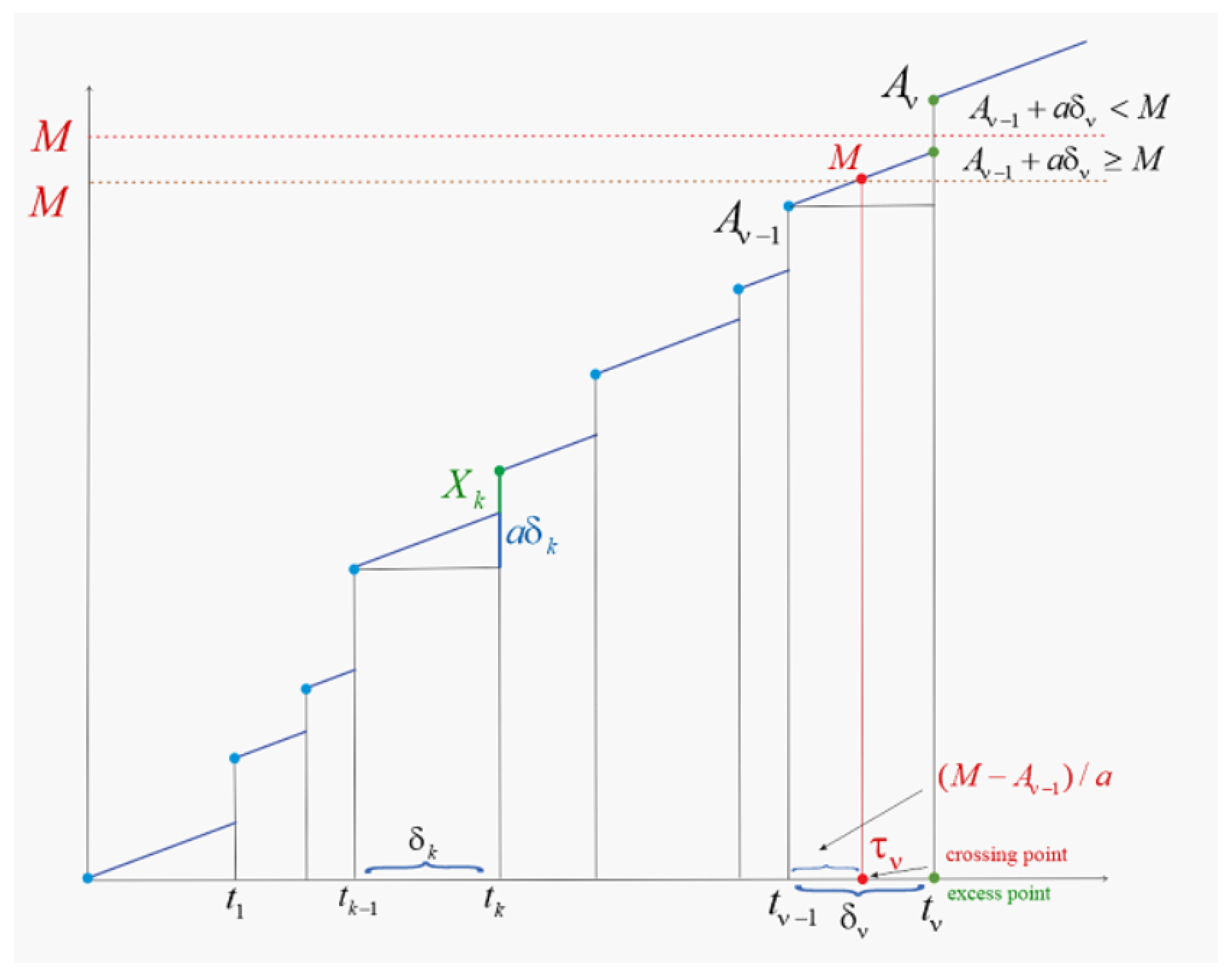
From the Figure 1, the failure can take place at the crossing of M or by an excess.

Figure 1.
The linear degradation process with shocks.
Namely, if , then the crossing takes place in interval with crossing at time , so that sharp. If , then the crossing of the horizontal line of height M takes place exactly at time (the th shock) exceeding M and valued at . Thus, is the excess level of cumulative damage above threshold M. The location of can be arbitrarily higher than M (in reality, process runs downhill and it can hit zero at worst).
1.3.1. Our Methodology
Our techniques fall into the category of fluctuation theory in the context of random walk processes. However, our model is far from a classical random walk where a generic particle or walker moves along a d-dimensional rectangular deterministic integer grid (also known as a lattice). The walker moves along all possible directions with equal probability and only one step at the time. It is placed in a bounded closed subset B of and the associated problem is to find its escape location from that set B. In our present model, the walker moves along a randomly generated grid that is not even rectangular. (See more on different variants of random walks in Dshalalow and White [27].) Here, the walker moves in within a random rectangular set and it escapes at the random point or . (See the walker’s path in Figure 1).
The model as set is not very common in the context of random walks, although as far as grids, some walks allow looser configurations. Yet, this is a new identification of reliability models as random walks. Secondly, we apply and embellish the theory of fluctuations to arrive at analytically closed formulas and establish the main functional for the joint probability distribution of the first passage time (called so in fluctuation theory) and the position of walker or escape location associated with the failure time and the extent of the overall damage, respectively.
Our approach allows further generalizations by including other types of shocks. We earlier worked on multidimensional walks (cf. Dshalalow and White [27]), only this time the walker’s movements are not rectangular. The present paper points to ways of their modifications.
1.3.2. Paper’s Layout
The paper is organized as follows. In Section 2, we formalize the system with a linear degradation process combined with cumulative shock model of non-fatal shocks arriving according to a general marked point process with position dependent marking that we introduced in the beginning of this section. We use an approach previously developed by the authors in [5,6,7] for a pure cumulative shock model but then expressed in terms of a random walk using fluctuation analysis. In this case, the model embellished by the presence of a degradation process required a quite different analysis, but still within the framework of the theory of fluctuations. We obtained a closed form functional of the joint distribution of the time failure and the detriment of the damage to the system, among other useful characteristics, like the status of the system on the shock preceding the fatal one or before the real crossing of the critical threshold. In Section 3, we support our claim of analytical tractability of the results by discussing a special case of the of a marked Poisson process with exponentially distributed marks. The results are confirmed through a comparison with simulation in Section 4.
2. Fluctuation Analysis of the Linear Degradation Process with Shocks
Consider a piece of equipment that ages and degrades at a deterministic rate a of damage per unit time, eventually degrading to a point that it becomes unuseful when its accumulated damage crosses a positive threshold M. In this idealized scenario, this occurs precisely at time . Practically, however, the piece of equipment deteriorates much faster due to occasional irreversible shocks of random magnitudes occurring at random times , which together form a marked point process. Estimating the crossing time of M and excess level of a marked point process crossing M by a piecewise constant jump process is a familiar task in the literature, but combining this with deterministic degradation poses a more challenging problem. The question is when the failure takes place and to what detriment. The latter may be of interest if the condition of the device is degraded beyond any repair.
In the context of the shock random measure (introduced in subsection Our Model of Section 1), we assume that the support counting measure represents a renewal process. That is, the times between consecutive shocks
are i.i.d. for and assuming . Then, the cumulative damage due to continual degradation and periodic shocks is
with being the associated continuous time parameter counting process describing the status of damage at any time t. Note that is not assumed to be with position independent marking, implying that the marks and are not independent for any fixed k but the vectors , are i.i.d. with a common joint Laplace–Stieltjes transform (LST)
which is assumed to be known or at least not difficult to estimate. With
define
the minimum number of shocks that along with degradation leads to the failure.
The failure time is and it can be one of the two values. It either equals if there no failure in interval or it is if the failure takes place in . Thus,
We denote by the failure damage of upon the failure time . It obviously is
We target the joint LST of the joint distribution of the failure time , the total damage to the system upon its failure (that is the crossing level), the pre-failure time (the time of the st shock preceding the failure), and the total damage to the system brought by the th shock. Note that is not the biggest damage prior to the failure unless . The last two parameters can be of independent interest. Thus,
Theorem 3.
The joint LST of the degradation upon the shock before the failure, the damage upon failure, the time of the shock before the failure, and the failure time satisfies
where
Proof.
First, we introduce a set of failure indices so that , which creates a set of functionals . We will derive an expression for and then use operational calculus to find a formula for .
The functional can be computed as a convenient partition of the sample space. The partition includes two subsets. First is the set of events where and is given, i.e., the failure occurs between the th and jth shocks as a result of the constant degradation, which we call a degradation failure. Formally,
Second is the set of events where and is given, i.e., the failure occurs upon the jth shock, which we call a shock failure. Formally,
Therefore, we have
The first expression, corresponding to the degradation failure, simplifies to
Next, we apply a modified Laplace transform to acting on variable p, which bypasses all terms except those that depend on p,
Therefore, we have
Then,
which completes the proof for Formula (43).
The second expression, corresponding to the shock failure, simplifies as
Next, we apply a different modified Laplace transform to acting on variable p, which bypasses all terms except those that depend on p,
Therefore, we have
Then,
as a geometric series, which establishes Formula (44).
Therefore, applying the inverse operators evaluated at the true threshold M yields
as required. □
In the following section, we will make some assumptions about the deterioration process to demonstrate the previous theorem can be applied to realistic special cases to find explicit probabilistic results about the deterioration.
3. Results for a Dual-Exponential Shock Process
To justify our claim for analytical tractability, we consider a special case under the following assumptions. Suppose the times between each shock are exponentially distributed with parameter and damage due to each shock being independent of each other. Using the terminology of random measures, the marked point process is with position independent marking. Then,
Suppose further that the times are exponentially distributed with parameter and the damage due to the shocks are exponentially distributed with parameter . Then,
In this special case, we establish an explicit formula for .
Proposition 1.
For the marked point process of the evolution of deterioration, let have position independent marking. Furthermore, if the times between shocks are exponentially distributed with parameter λ and the impacts of the shocks ’s are exponentially distributed with parameter μ, then the joint LST of the deterioration upon the shock before the failure, the deterioration upon failure, the time of the shock before the failure, and the failure time satisfies
where
and
under the notation
where and are the roots of the polynomial and is the discriminant of the polynomial, with
and
Proof.
For the first term from Theorem 3, notice
As we see, this is simply a rational function with degree 2 (in x) in the numerator and degree 3 in the denominator, which means the inverse Laplace transform can be computed easily with a partial fraction decomposition to find
Similarly,
This is, again, a rational expression—this time with degree 4 in the denominator, so its inverse Laplace transform can be computed easily with a partial fraction decomposition to find
The result above is a very information-rich functional in this special case and can give us expressions for many interesting probabilistic results. We outline a few such results below. First, the probability of failure occurring between shocks and probability of failure upon a shock.
Corollary 1.
Under the assumptions of Proposition 1, the probabilities of degradation failure and shock failure are
and
Proof.
For the probability of a degradation failure, simply let in to find
For the probability of shock failure, simply let in to find
□
Interestingly, as the threshold M grows, the probabilities approach constants and . Of course, the sum of the probabilities is 1 since exactly one of these disjoint events will almost surely occur.
Corollary 2.
Under the assumptions of Proposition 1, the marginal LST of the failure time is
This LST can easily yield means and moments, as we see below.
Proposition 2.
Under the assumptions of Proposition 1, the mean and variance of the failure time are
and
Proof.
The first two moments of can readily be found by taking the first two derivatives of , managing the signs appropriately and taking limits, yielding the results above. □
Let us now consider the failure damage of the process.
Corollary 3.
Under the assumptions of Proposition 1, the marginal LST of the failure damage is
Proof.
Let , then
The first term simplifies to
and the second term simplifies to
Next, we use the LST of to find simple explicit formulas of its mean and variance.
Corollary 4.
Under the assumptions of Proposition 1, the mean and variance of the failure damage are
and
Proof.
The first two moments of can readily be found by taking the first two derivatives of , managing the sign appropriately and taking limits, yielding the results above. □
These results reveal a number of intuitive facts. The mean of makes clear the obvious fact that the failure damage will always be at least M, but more interestingly shows that the excess of the failure damage is precisely (shock failure), the mean time between shocks multiplied by the probability of a shock failure, meaning it cannot surpass the mean time between shocks. In addition, as M grows, the mean approaches M as shocks become small relative to M and the variance approaches the constant .
4. Comparison with Stochastic Simulation
In this section, predictions from the formulas for probabilities, means, and variances derived for the exponential special case in the previous section will be shown to agree with Monte Carlo simulation of the process under numerical assumptions on the parameters: the degradation rate a, the parameter of the exponentially distributed time between shocks , the parameter of the exponentially distributed shock damage , and the threshold M.
Simulation code is written in the Python language with the NumPy library for numerical computation. The code for simulating paths of the process has been included in Appendix A along with diagrams and a description of the code. The experiments run in this section have been made available publicly by the authors online: see the Data Availability Statement of this article.
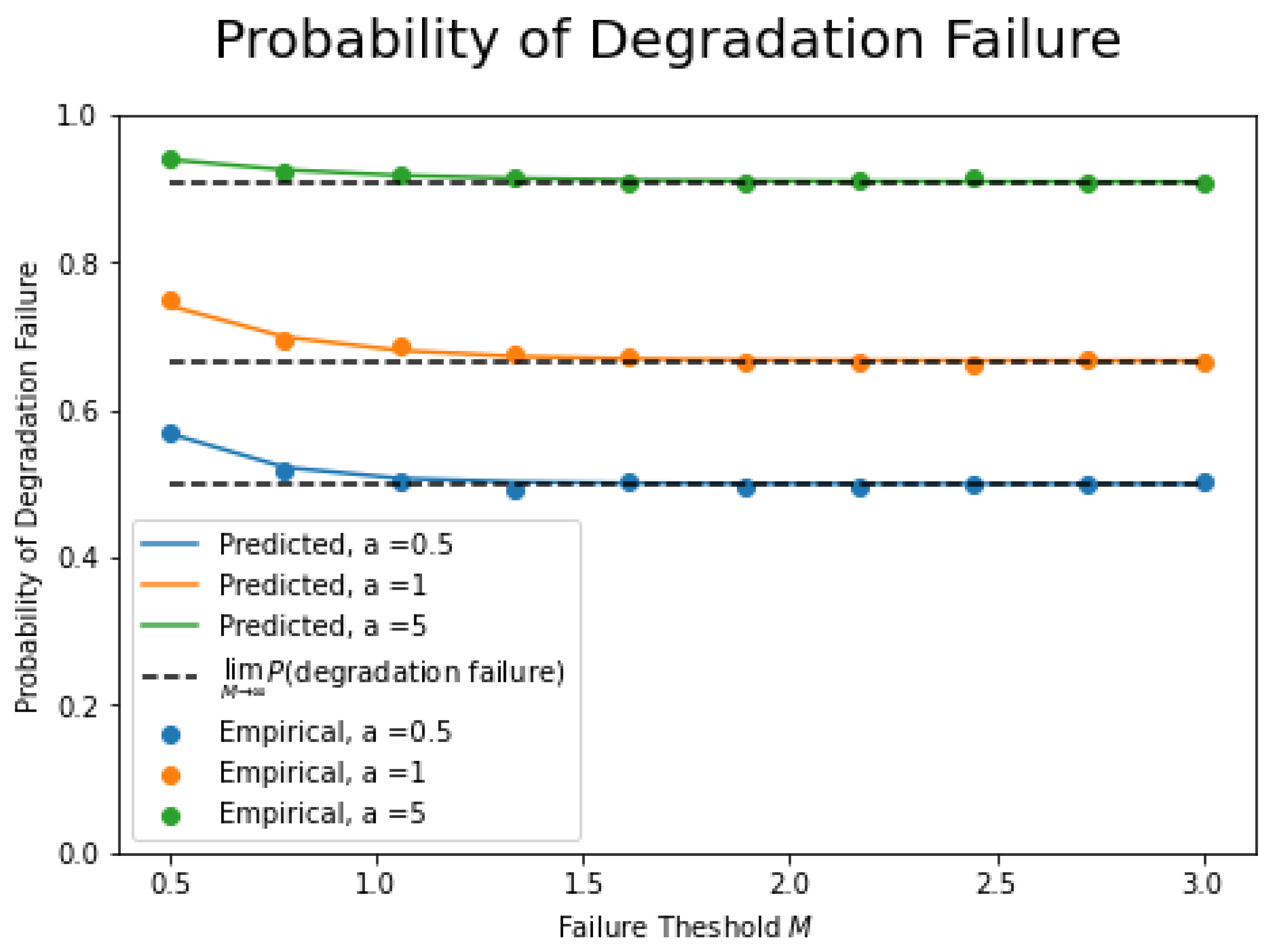
Suppose and . Figure 2 below focuses on the probability of a degradation failure (rather than a shock failure). The curves correspond to the predictions for probability of degradation failure from Corollary 1, while the dots represent empirical probabilities corresponding to simulations of 10,000 paths of the process for each pair of parameters .
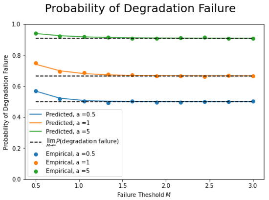
Figure 2.
Predicted and empirical probabilities of degradation failures with limiting probabilities.
Notice the degradation failure probabilities have an inverse relationship with the threshold M as a quick degradation failure become less probable and shocks become increasingly probable causes of failures. Further, we plotted the limiting probabilities as dotted horizontal lines of height and note the probabilities all approach these, as predicted. Further, probabilities are inversely related the degradation rate a. Clearly, this confirms the intuitive fact that a higher degradation rate should result in more degradation failures.
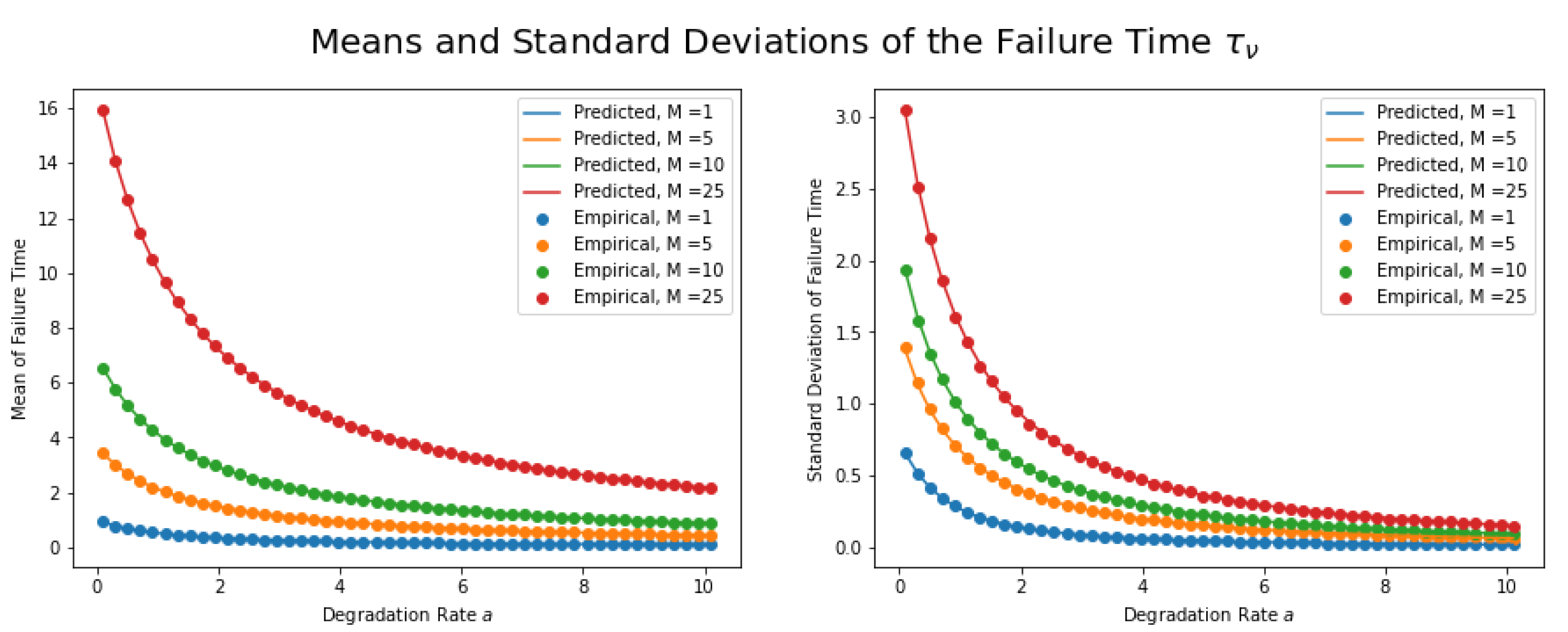
Suppose and . Figure 3 below focuses on the mean and variance of the failure time . The curves correspond to the predictions for the mean and standard deviation from Proposition 2, while the dots represent empirical means and standard deviations corresponding to simulations of 10,000 paths of the process for each pair of parameters .
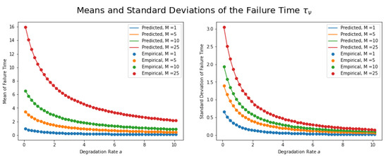
Figure 3.
Predicted and empirical values for the mean and standard deviation of the failure time.
Note that the mean failure time shrinks as the degradation rate a grows and failures occur more quickly while the threshold M and mean failure time have a positive relationship as failures occur more slowly. We see similar trends with the standard deviation: variability decreases as the degradation rate grows and the deterministic part of the degradation is more influential while variability grows as the threshold grows and more shocks will typically occur in paths.
Suppose that and . Figure 4 below focuses on the failure damage . The curves correspond to the predictions for the mean and standard deviation from Proposition 4, while the dots represent empirical means and standard deviations corresponding to simulations of 1,000,000 paths of the process for each pair of parameters . (Note we generated more paths in this case because the empirical standard deviations took longer to converge to the true predicted values.)
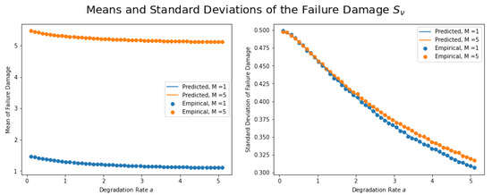
Figure 4.
Predicted and empirical values for the mean and standard deviation of the failure damage.
Here, as degradation rate grows, we saw that shock failures become less probable previously, which causes the mean failure damage to decrease toward M, as degradation failures with positions equal to M sharp are more likely. The standard deviation of failure damage has an inverse relationship with a and a positive relationship with M for reasons analogous to the same trends in the mean failure time.
5. Conclusions
In this paper, we studied a reliability system with linear degradation and external shocks (cumulative shocks model with degradation) that further accelerate its deterioration and lead to an inevitable failure (soft failure) when the overall degradation crosses or exceeds an M, its sustainability threshold. The gradual degradation and random damages to the system can be modeled by a random walk type process, although not in the classical sense where a walker moves along a rectangular grid. In a more recent work, random walk is considered on a variety of configurations, more general than rectangular, cf. Dshalalow and White [27]. Now the random walk modeling is not just an interpretation, but it suggested fluctuation analysis as a primary tool for dealing with this class of models, with the benefit of obtaining a closed form distribution of targeted parameters such as the failure time of the system and the total damage to the system at the failure time. The latter is noteworthy information in the event the targeted component can be repaired or completely discarded.
The time dependent status of degradation of the system can be formalized by the marked point random measure with position dependent marking. Here, is the arrival process of non-fatal shocks of respective magnitudes . The degradation is further enhanced by the random increment in interval where a is the constant degradation rate and is the length of the time interval . We allow to depend on as well, although in some special cases we can lift this assumption. No assumption is made about the nature of , and thus . Note that position dependent marking refers to the sequence which is comprised of independent vectors but with mutually dependent components. The system fails at some random time when the continuous time parameter degradation process crosses or exceeds some M. Note that the crossing of M can occur upon one of the arriving shocks at , say at or within the interval that we associate with a time . The overall damage to the system upon its failure is measured by the quantity being M sharp or dependent on whether or .
We targeted the joint transform that carries two more quantities, and , giving us information about the system upon a shock preceding the time of failure. We arrived (Section 2) at the formula
where
is the joint transform of and , which is supposed to be known once we specify the and , and is the inverse Laplace transform in variable x.
To support our claim that the above formula is closed form, we considered in Section 3 a special case of position independent marking and the assumptions on and as being exponential. Under these assumptions, the respective transforms were inverted in a rather compact formula, further extended by marginal distributions of the failure time and the failure damage , and their means and variances. In Section 4, we presented numerical results for several concrete numbers and compared them with simulated results which all agreed.
The overall results are explicit, general, and use fluctuation techniques different from the mainstream literature. The approach allows us to further embellish the current system making it a series system of two or more components applying and embellishing previously developed techniques of stochastic games (Dshalalow [28]).
Author Contributions
Conceptualization, J.H.D.; methodology, J.H.D. and R.T.W.; validation, R.T.W.; formal analysis, J.H.D. and R.T.W.; investigation, J.H.D. and R.T.W.; writing—original draft preparation, J.H.D. and R.T.W.; writing—review and editing, J.H.D. and R.T.W.; visualization, J.H.D. and R.T.W. Both authors have read and agreed to the published version of the manuscript.
Funding
This research received no external funding.
Data Availability Statement
The authors have made all code and simulated datasets used in the paper can be found in the the GitHub repository https://github.com/rtwhite1546/ShockDegradationModel, accessed on 18 August 2021.
Acknowledgments
The authors are indebted to anonymous referees whose insightful comments and suggestions contributed a great deal of improvement to the clarity and presentation of our work.
Conflicts of Interest
The authors declare no conflict of interest.
Abbreviations
The following abbreviations are used in this manuscript:
| General Acronyms | |
| i.i.d. | independent and identically distributed |
| LST | Laplace-Stieltjes transform |
| probability distribution function | |
| probability density function | |
| PGF | probability-generating function |
| r.v. | random variable |
| Notation in the Literature Review | |
| soft shocks marked point process in cumulative shock model | |
| associated support counting measure of shocks’ arrivals | |
| the number of shocks in time interval | |
| Dirac point mass (unity measure) | |
| magnitudes of soft shocks | |
| the time of the nth shock | |
| pure degradation process | |
| magnitudes of hard shocks | |
| marked point measure of hard shocks | |
| lower threshold in -shock policy models | |
| x | failure threshold |
| M | soft failure threshold |
| D | hard failure threshold |
| number of soft shocks until soft failure with respect to threshold x | |
| number of hard shocks until hard failure with respect to threshold x | |
| A | the set that process escapes |
| Notation in Our Model | |
| number of the first shock where degradation exceeds M | |
| pre-failure time | |
| soft failure time (the escape from set A) | |
| pre-failure cumulative damage | |
| cumulative damage to the system at the failure | |
| operator | |
| modified Bessel function of order zero | |
| soft shocks and degradation marked point process | |
| cumulative degradation process including shocks | |
| M | failure threshold |
| failure time if it occurs upon constant degradation | |
| failure time if it occurs upon a shock | |
| Laplace transform | |
| inverse Laplace transform | |
| p | failure threshold |
| standard Gaussian PDF | |
| equivalence class of all exponential distributions with parameter | |
| equivalence classs of all geometric random variables with parameter | |
| equivalence class of all gamma distributions with parameters | |
| equivalence class of all Gaussian distributions with parameters | |
Appendix A
Appendix A.1. Simulation Code
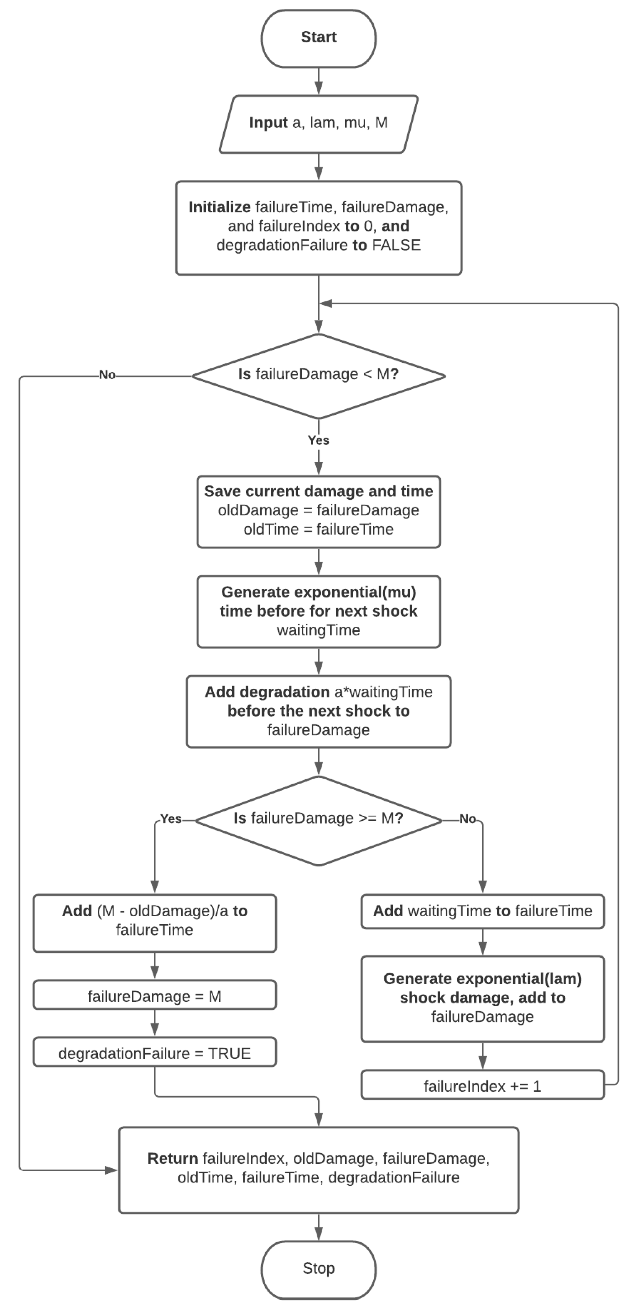
Simulation code was written in Python using the NumPy library. First, we created a function simulatePath that takes the parameters of the process as inputs, simulates the process until a failure occurs, and returns the four terms in the functional , i.e., the failure index , damage upon the shock before the failure , the failure damage , the time of the shock before the failure , and the failure time as well as a Boolean flag indicating a degradation failure (if TRUE) or shock failure (if FALSE).
Figure A1 is a flow chart describing how the simulation proceeds.
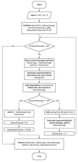
Figure A1.
The simulatePath function accepts numerical inputs for each parameter of the process: a, , , and M. It then simulates one path of the process and returns sampled values of , , , and along with a flag indicating whether a degradation failure or shock failure occurred.
Figure A1.
The simulatePath function accepts numerical inputs for each parameter of the process: a, , , and M. It then simulates one path of the process and returns sampled values of , , , and along with a flag indicating whether a degradation failure or shock failure occurred.
Next is the full Python code for the simulatePath function.
- import numpy as~np
- def simulatePath(a, lam, mu, M):
- # initialize outputs
- failureTime = 0
- failureDamage = 0
- failureIndex = 0
- degradationFailure = False
- # simulate the process
- while failureDamage < M:
- # save A_j-1
- oldDamage = failureDamage
- # save t_j-1
- oldTime = failureTime
- # compute waiting time before the next shock
- waitingTime = np.random.exponential(1/mu)
- # add degradation between shocks
- failureDamage += a ∗ waitingTime
- # if degradation causes damage to reach M...
- if failureDamage >= M:
- # compute tau_nu
- failureTime += (M - oldDamage)/a
- # set S_nu (total damage) to M
- failureDamage = M
- # mark degradation as the cause of the failure
- degradationFailure = True
- # exit the loop
- break
- # else, add the shock
- else:
- # add the waiting time
- failureTime += waitingTime
- # add the shock damage
- failureDamage += np.random.exponential(1/lam)
- # add 1 to the shock counter
- failureIndex += 1
- # gather the output values into a tuple
- outputs = (failureIndex, oldDamage, failureDamage,
- oldTime, failureTime, degradationFailure)
- # return values nu, A_nu-1, S_nu, t_nu-1, tau_nu, flag for
- # failure type
- return outputs
Then, a single path of the process can be simulated with the command
- simulatePath(a, lam, mu, M)
for any parameters one chooses. All empirical results in Section 4 are created by generating many paths of the deterioration process with this function and finding means and variances of the outputs across generated paths.
The formulas derived in Corollary 1, Proposition 2, and Proposition 4 were implemented as the following Python functions to compute predicted results.
- def degradationProbability(a, lam, mu, M):
- term = a ∗ lam + mu ∗ np.exp(-(lam + mu / a) ∗ M)
- return term / (a ∗ lam + mu)
- def failureTimeMean(a, lam, mu, M):
- term = lam ∗ M + 1 - degradationProbability(a, lam, mu, M)
- return term / (a ∗ lam + mu)
- def failureTimeVariance(a, lam, mu, M):
- dTerm = a ∗ lam + mu
- eTerm = np.exp(-(lam + mu / a) ∗ M)
- term1 = 2 ∗ lam ∗ mu ∗ M / dTerm ∗∗ 3
- term2 = mu ∗ (mu - 4 ∗ a ∗ lam) / dTerm ∗∗ 4
- term3 = 2 ∗ mu
- term3 ∗= 2 ∗ a ∗∗ 2 ∗ lam + (a ∗ lam) ∗∗ 2 ∗ M - 2 ∗ mu ∗∗ 2 ∗ M
- term3 ∗= eTerm / (a ∗ dTerm ∗∗ 4)
- term4 = 2 ∗ mu ∗∗ 2 ∗ eTerm ∗∗ 2 / dTerm ∗∗ 4
- return term1 + term2 + term3 - term4
- def failureDamageMean(a, lam, mu, M):
- return M + (1 - degradationProbability(a, lam, mu, M)) / lam
- def failureDamageVariance(a, lam, mu, M):
- dTerm = a ∗ lam + mu
- eTerm = np.exp(-(lam + mu / a) ∗ M)
- term1 = 2 ∗ a ∗ mu ∗ (1 - eTerm) / (lam ∗ dTerm ∗∗ 2)
- term2 = mu ∗∗ 2 ∗ (1 - eTerm ∗∗ 2) / (lam ∗ dTerm) ∗∗ 2
- return term1 + term2
References
- Tsai, C.C.; Tseng, S.T.; Balakrishnan, N. Mis-specification analyses of gamma and Wiener degradation processes. J. Stat. Plan. Inference 2011, 141, 3725–3735. [Google Scholar] [CrossRef]
- Gut, A. Cumulative shock models. Adv. Appl. Probab. 1990, 22, 504–507. [Google Scholar] [CrossRef] [Green Version]
- Gut, A.; Hüsler, J. Shock models. In Advances in Degradation Modeling: Applications to Reliability, Survival Analysis, and Finance; Nikulin, M.S., Limnios, N., Balakrishnan, N., Kahle, W., Huber-Carol, C., Eds.; Springer: Berlin/Heidelberg, Germany, 2010; Chapter 5; pp. 56–124. [Google Scholar]
- Sumita, U.; Shanthikumar, J.G. A class of correlated cumulative shock models. Adv. Appl. Probab. 1985, 17, 347–366. [Google Scholar] [CrossRef]
- Abolnikov, L.; Dshalalow, J.H. A first passage problem and its applications to the analysis of a class of stochastic models. J. Appl. Math. Stoch. Anal. 1992, 5, 83–97. [Google Scholar] [CrossRef] [Green Version]
- Dshalalow, J.H.; Huang, W. On noncooperative hybrid stochastic games. Nonlinear Anal. Hybrid Syst. 2008, 2, 803–811. [Google Scholar] [CrossRef]
- Dshalalow, J.H.; Robinson, R. On one-sided stochastic games and their applications to finance. Stoch. Model. 2012, 28, 1–14. [Google Scholar] [CrossRef]
- Gut, A.; Hüsler, J. Extreme shock models. Extremes 1999, 2, 295–307. [Google Scholar] [CrossRef]
- Li, Z.; Kong, X. Life behavior of δ-shock model. Stat. Probab. Lett. 2007, 77, 577–587. [Google Scholar] [CrossRef]
- Eryilmaz, S.; Bayramoglu, K. Life behavior of δ-shock models for uniformly distributed interarrival times. Stat. Pap. 2013, 55, 841–852. [Google Scholar] [CrossRef]
- Eryılmaz, S. Generalized δ-shock model via runs. Stat. Probab. Lett. 2012, 82, 326–331. [Google Scholar] [CrossRef]
- Mallor, F.; Omey, E. Shocks, runs and random sums. J. Appl. Probab. 2001, 38, 438–448. [Google Scholar] [CrossRef]
- Mallor, F.; Santos, J. Reliability of systems subject to shocks with a stochastic dependence for the damages. Test 2003, 12, 427–444. [Google Scholar] [CrossRef]
- Mallor, F.; Omey, E.; Santos, J. Asymptotic results for a run and cumulative mixed shock model. J. Math. Sci. 2006, 138, 5410–5414. [Google Scholar] [CrossRef]
- Ozkut, M.; Eryilmaz, S. Reliability analysis under Marshall–Olkin run shock model. J. Comput. Appl. Math. 2019, 349, 52–59. [Google Scholar] [CrossRef]
- Marshall, A.W.; Olkin, I. A multivariate exponential distribution. J. Am. Stat. Assoc. 1967, 62, 30–44. [Google Scholar] [CrossRef]
- Marshall, A.W.; Olkin, I. A generalized bivariate exponential distribution. J. Appl. Probab. 1967, 4, 291–302. [Google Scholar] [CrossRef]
- Eryilmaz, S.; Tekin, M. Reliability evaluation of a system under a mixed shock model. J. Comput. Appl. Math. 2019, 352, 255–261. [Google Scholar] [CrossRef]
- Zhao, X.; Guo, X.; Wang, X. Reliability and maintenance policies for a two-stage shock model with self-healing mechanism. Reliab. Eng. Syst. Saf. 2018, 172, 185–194. [Google Scholar] [CrossRef]
- Peng, H.; Feng, Q.; Coit, D.W. Reliability and maintenance modeling for systems subject to multiple dependent competing failure processes. IIE Trans. 2010, 43, 12–22. [Google Scholar] [CrossRef]
- Hao, H.; Su, C.; Qu, Z. Reliability analysis for mechanical components subject to degradation process and random shock with Wiener process. In The 19th International Conference on Industrial Engineering and Engineering Management; Springer: Berlin/Heidelberg, Germany, 2013; pp. 531–543. [Google Scholar] [CrossRef]
- Rafiee, K.; Feng, Q.; Coit, D.W. Reliability assessment of competing risks with generalized mixed shock models. Reliab. Eng. Syst. Saf. 2017, 159, 1–11. [Google Scholar] [CrossRef] [Green Version]
- Hao, S.; Yang, J.; Ma, X.; Zhao, Y. Reliability modeling for mutually dependent competing failure processes due to degradation and random shocks. Appl. Math. Model. 2017, 51, 232–249. [Google Scholar] [CrossRef]
- Yousefi, N.; Coit, D.W.; Song, S.; Feng, Q. Optimization of on-condition thresholds for a system of degrading components with competing dependent failure processes. Reliab. Eng. Syst. Saf. 2019, 192, 106547. [Google Scholar] [CrossRef] [Green Version]
- Cao, Y.; Liu, S.; Fang, Z.; Dong, W. Modeling ageing effects in the context of continuous degradation and random shock. Comput. Ind. Eng. 2020, 145, 106539. [Google Scholar] [CrossRef]
- Oliveira, R.P.; Achcar, J.A.; Mazucheli, J.; Bertoli, W. A new class of bivariate Lindley distributions based on stress and shock models and some of their reliability properties. Reliab. Eng. Syst. Saf. 2021, 211, 107528. [Google Scholar] [CrossRef]
- Dshalalow, J.H.; White, R.T. Current trends in random walks on random lattices. Mathematics 2021, 9, 1148. [Google Scholar] [CrossRef]
- Dshalalow, J.H. On the level crossing of multi-dimensional delayed renewal processes. J. Appl. Math. Stoch. Anal. 1997, 10, 355–361. [Google Scholar] [CrossRef] [Green Version]

Publisher’s Note: MDPI stays neutral with regard to jurisdictional claims in published maps and institutional affiliations. |
© 2021 by the authors. Licensee MDPI, Basel, Switzerland. This article is an open access article distributed under the terms and conditions of the Creative Commons Attribution (CC BY) license (https://creativecommons.org/licenses/by/4.0/).