Abstract
In the field of education, the assessment of a student’s learning performance is based on his final course scores. Few people care about what is behind the numbers. Most of the time, the final scores represent the end of the course because students have already passed the subject. Low-level students especially, still have a lot of misconceptions, but they do not know how to make up for their poor grasp of the subject in preparation for future study. Instead of just giving students their scores, teachers are encouraged to provide remedial instruction to students for their future learning. This study aims to establish an effective method using rough set theory and grey structural modeling to determine which attributes affect students’ final scores and to cluster students accordingly. A rough set algorithm generates a set of attributes for an assessment list. Grey structural modeling (GSM) is then used to cluster students who have the same weaknesses in English. GSM changes from one dimension to two dimensions, and calculates the relative distance, so that cluster analysis can be performed. Targeted remedial instruction can then be given to each similar ability student grouping. The results revealed that through integrating the two theories, teachers could more effectively sort students into groups. Students benefit by coming to understand their weaknesses in English instead of just receiving a single score at the end of the semester, and they can learn with their peers as well. Teachers can adjust their teaching strategies and syllabus design based on the analytical results to target the students’ needs.
MSC:
20D05
1. Introduction
In the basic mode of teaching, the teaching process is divided into four parts: teaching goals, pre-assessment, teaching activities, and assessment. Assessment is often regarded as the last stage in the process; however, it does not mean the end of the teaching or learning. Assessment is a process of collecting information, forming judgments and then making decisions [1,2]. Throughout the teaching process, assessment has the function of undertaking transformation and providing feedback [3]. That is, the results of assessment can provide feedback to both teachers and students. Effective students monitor themselves and form internal feedback while less effective ones depend on their teachers for feedback [3]. In other words, the main purpose of assessment is to analyze whether teaching goals have been attained and to diagnose learning difficulties. Moreover, remedial instruction can be implemented based on the assessment results. However, this might be a problem because there are individual differences in students’ learning. How then can the teacher give the students the same remedial instruction based solely on their final scores rather than addressing their real weaknesses?
Traditional test assessments include many uncertain factors, and the item response theory (IRT), due to its basic assumptions, requires large sample sizes for test analysis [4]. However, in actuality, it is difficult to obtain large sample sizes, so the application range of IRT has its limitations. In view of this, the current study chose to use grey system theory because it needs only a small sample size to reach a considerable degree of assessment accuracy [5,6,7]. Grey system theory, put forward by Deng Julong in 1982, has as its theoretical basis the need to conduct correlation analysis for ambiguous or incomplete systems [6,7]. In order to cluster students with the same misconceptions, grey structural modeling (GSM) from grey system theory was used to carry out the matrix arrangement of student assessments, and then to perform cluster analysis [8,9]. There are two main reasons for adopting GSM in clustering in this research study, the first being that the number of samples is small. The second is because a key characteristic of grey system theory is its ability to analyze the known minimum amount of information despite small samples lacking in information and having other issues of uncertainty. This is different from traditional statistical analysis methods that require large samples.
In addition, the study also used rough set theory to discover the weighting of the attributes affecting students’ final scores. Rough set theory, proposed by Pawlak, has advantage of being able to obtain the same knowledge as the original decision–making system without losing any information, and without obeying any assumptions [10,11,12]. The main purpose of rough set theory is to extract rules from an information system composed of an object and its corresponding attribute factors that are sufficient to describe under which attribute conditions an object should be classified [10,11,12].
The study is based on a sample of 29 students enrolled in the same freshman English class for two semesters in one academic year. All of them are low-level students whose English ability is considered to be at the CEFR A2 level. They need to do the assigned tasks in and after class. The midterm and final exams are comprised of similar tasks as those assigned. Hence, the better students can perform the assigned tasks, the higher the scores they will attain on their midterm and final exams. If the teacher can find the attribute weighting of these assigned tasks that affects students’ learning outcomes and provide remedial instruction in time, students will be able to learn English more effectively. Remedial instruction in this study refers to 15-min group remedial learning that lasts for 10 weeks during the second semester.
The purpose of the study is to integrate rough set theory and GSM to establish effective remedial instruction. Students usually receive their final scores at the end of the semester; however, the final scores should not mean the end of learning. Knowing what is behind the numbers how it can be used to benefit students in their future learning is more important than the final scores. However, if the students are divided into groups based on the teacher’s observations, they will sometimes ask, “Why should I belong to this group?” Therefore, the study integrated rough set theory and GSM to determine which attributes influence students’ final scores most, and then cluster students into different groups for remedial instruction. Different sets of remedial instruction can be designed to fit each group. Students will also benefit from social learning made possible by being grouped with their true peers as they learn to collaborate, respect, learn, accept, and support each other during the cooperative learning process. With the purpose of providing effective remedial instruction to different student groups, the study aims to answer the following research questions:
- (1)
- What tasks attribute influences students most in their overall English performance?
- (2)
- How can students be clustered into same level groups and given effective remedial instruction?
2. Methodology
In this section, cluster analysis methods, rough set theory and grey structural modeling are introduced.
2.1. Cluster Analysis Methods
Cluster analysis, proposed by Sokal and Sneath in 1963, is another kind of multivariate analysis which aims to divide data objects into several groups based on how closely associated they are [13]. When the objects are not all homogeneous, cluster analysis is a very useful technique in data analysis. After cluster analysis and grouping, the objects within a group will be consistent for certain characteristics while the objects belonging to different groups will be significantly different for the same characteristics [14,15]. Based on the definition above, cluster analysis can be applied to many fields such as finance, marketing, politics, and education. Based on the concept of cluster analysis, the students in this study were clustered according to their English learning performance for the purpose of facilitating remedial teaching.
The commonly used clustering indicators are distance and similarity coefficients [16]. In research, data having the shortest distance and greatest similarity are generally lumped into the same group. In structural clustering, choosing the distance to be measured is the most critical step. A simple method of determining this measurement to use is Manhattan distance, which is equivalent to the sum of the absolute differences between two vectors. It is the distance a taxi cab would have to travel on a grid of city streets to travel from Point A to Point B. Euclidean distance is the shortest distance between two points as the crow flies. In this study, Minkowski distance, a generalization of Euclidean distance and Manhattan distance, is used in grey structural modeling.
There are basically three cluster analysis methods [17]. The first is hierarchical clustering, which uses a hierarchical structure or a tree structure to describe the clustering process. The second is the non-hierarchical clustering, also known as stepwise clustering or K-means clustering. The remaining alternative is two-stage clustering, a combination of the first two methods of hierarchical clustering and non-hierarchical clustering. In two-stage clustering, first, Ward’s method or other hierarchical clustering method is used for grouping. After determining the number of cluster groups, K-means clustering is used to move individuals within groups. If the number of observations is large or the data file is very large (more than 200), it is more appropriate to use K-means clustering. Otherwise, a hierarchical cluster analysis method is more appropriate for grouping. Since this research had only a small sample, the grey structural modeling hierarchical analysis method for clustering students’ performance was used.
2.2. Rough Set Theory
Pawlak formed rough sets by assigning objects related to the confirmation of ideas that fell within the boundary line region, which is defined as the difference set between the upper and lower approximation sets [10,11,12]. Because rough sets can be described by explicit mathematical formulas, the number of fuzzy set elements can be calculated (i.e., the fuzziness between 0 and 1 can be determined through calculation) [10,11,12]. This feature offers an effective means of dealing with the routine nature of unclear problems and managing uncertainty with incomplete information or knowledge.
In mathematical terms, rough sets use lower and upper approximation sets to classify data based on imprecise results, both observed and measured, without any prior assumptions or additional relevant data information (a key problem in reasoning, learning, and decision making) [18,19,20,21,22]. Rough set theory has a wide range of applications including medical engineering, process management, and financial engineering, and is currently used in three major domains: corporate bankruptcy forecasting, database marketing, and financial investment forecasting [20,21,22]. The main feature of rough set theory is that it can use historical databases (knowledge bases) to mine information for hidden models from which to predict the future, where historical databases of the aforementioned three domains are built from multiple attribute information tables and share similar predictive characteristics [20,21,22]. This study uses the characteristics of rough set theory to analyze the weights of the various attributes influencing the English final score as the theory can not only consider the methods of expressing, learning, and generalizing precise knowledge but also discover information from large amounts of data, infer knowledge, and discern systems.
2.3. Object of Study by Rough Sets
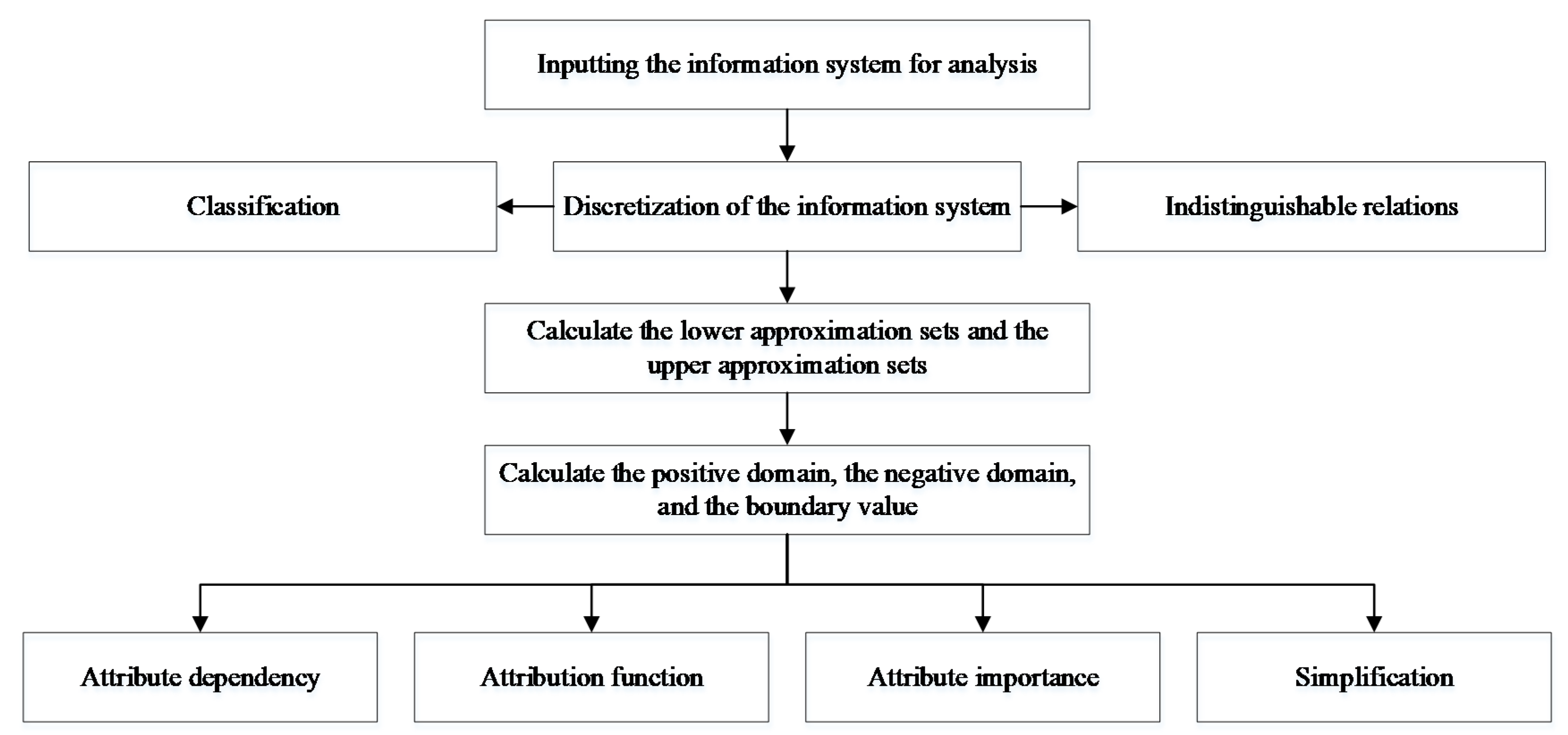
Because the starting point of problem solving using rough set theory is the indistinguishability of knowledge in information systems, the focus is on the roughness of a set [23,24,25]. Accordingly, rough set theory defines the set of equivalence classes of various equivalence relations as the rough set (also called the upper and lower approximation sets of a certain set of objects), and the main computational output is the expression and simplification of knowledge [21,22,23,24,25]. According to this description, we see that the object of study by rough sets is quite simple. In Figure 1, the object of study by rough sets is represented in the simplest graphical manner.
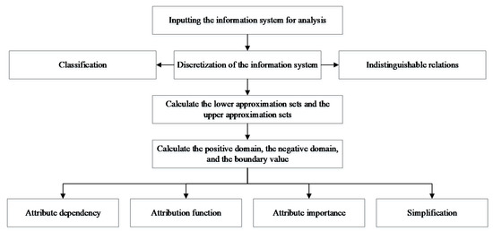
Figure 1.
Flow of the object of study on rough sets.
The mathematical model of the rough set used in this study consists of the following [23,24,25].
- (1)
- Information system (IS):where is a finite set of objects, and is the attribute set.
- (2)
- Information function:where is the set of values occurring in the attribute or in the domain of attribute . In simplest terms, is the correspondent value of the object in in terms of the attribute .
- (3)
- Discretization:
In decision-making problems, the attributes of internal information are often continuous. To use rough sets to analyze them, they must be transformed into discrete forms. Therefore, discretization of continuous attributes is the main premise of using rough sets [23,24,25].
Discretization is the mathematical transformation of continuous attributes into discrete forms. Essentially, this entails using subjectively selected breakpoints to divide the space constituted by conditional attributes, forming a finite number of regions, and ensuring the decision values of the objects in each region are the same [23,24,25]. To date, many methods are used for discretization of continuous attributes, and different discretization methods will produce different results. However, regardless of the method used, the following two requirements must be met [23,24,25]:
- (a)
- The spatial dimension following discretization should be reduced as much as possible (i.e., each attribute after discretization should be reduced to the minimum).
- (b)
- The amount of information lost after the discretization of attributes must be minimized.
Although many different discretization methods exist, the method of equal interval width discretization was used in this study.
Equal interval width discretization mainly divides the continuous attribute into k equally spaced regions subjectively. The mathematical model is:
where and are the maximum and minimum values of continuous attributes, respectively. In other words, the domain of the attribute values is .
After normalizing the discretization of the continuous attributes, a region for the attribute values can be obtained as:
where is the representative value after normalized discretization, and k is the grade of normalized discretization.
- (4)
- Upper and lower approximation sets
In a rough set, according to the definable set of attributes , for each set , the case of their indistinguishable equivalence classes can be examined. Let us assume the knowledge base is given. For each subset and a relationship of equivalence , set can be divided according to the description of basic set [24,25]. This definition of a rough set approximated by two exact sets is referred to as the upper and lower approximation sets [10,11], where the mathematical model of the lower approximation set is given as:
and the mathematical model of the upper approximation set is:
In simplest terms, use of attribute set R involves:
- (a)
- The lower approximation set, which represents the set of elements that are “fully (definitively)” classified as equal under all y decisions.
- (b)
- The upper approximation set, which represents the set of elements that are “possibly (any one of them)” classified as equal under all y decisions.
- (5)
- Positive, negative, and boundary under and [22,23,24,25]:
- (a)
- The positive domain of : the positive domain or the lower approximation set of , that is, , is the set of elements in that can be fully classified into set according to .
- (b)
- The negative domain of : the negative domain is the set of elements in that, according to , cannot be fully identified as belonging to the set , and it is the complement of .
- (c)
- Boundary: boundary is the set of elements that, according to knowledge and , cannot be fully identified as belonging to set nor to set , expressed in the following equation.
If , then X is called the boundary of the rough set; otherwise, no boundary exists. In addition, in terms of form, the upper approximation set is the union set of the positive and boundary domains. Therefore, it can be expressed as:
- (6)
- Attribute dependency
In the decision system, when it is assumed that C and D denote conditional and decision attributes, respectively, then the positive region of decision attributes under conditional attributes can be defined as [23,24,25]:
where is the set of objects that can be fully classified into the category under the division () according to knowledge C. “Attribute dependency ” represents the ratio of objects that can be fully classified in the decision under the condition of attribute C to the total number of objects in the set. In other words, this represents the degree of dependency of the decision attribute on the conditional attribute.
In a rough set, the dependency of decisional attribute D on conditional attribute C is defined as:
- (7)
- Significance of attributes
According to the dependency formula, the attribute importance is also defined in the rough set (i.e., in the decision system) [22,23,24]. Specifically, the attribute importance of is defined as:
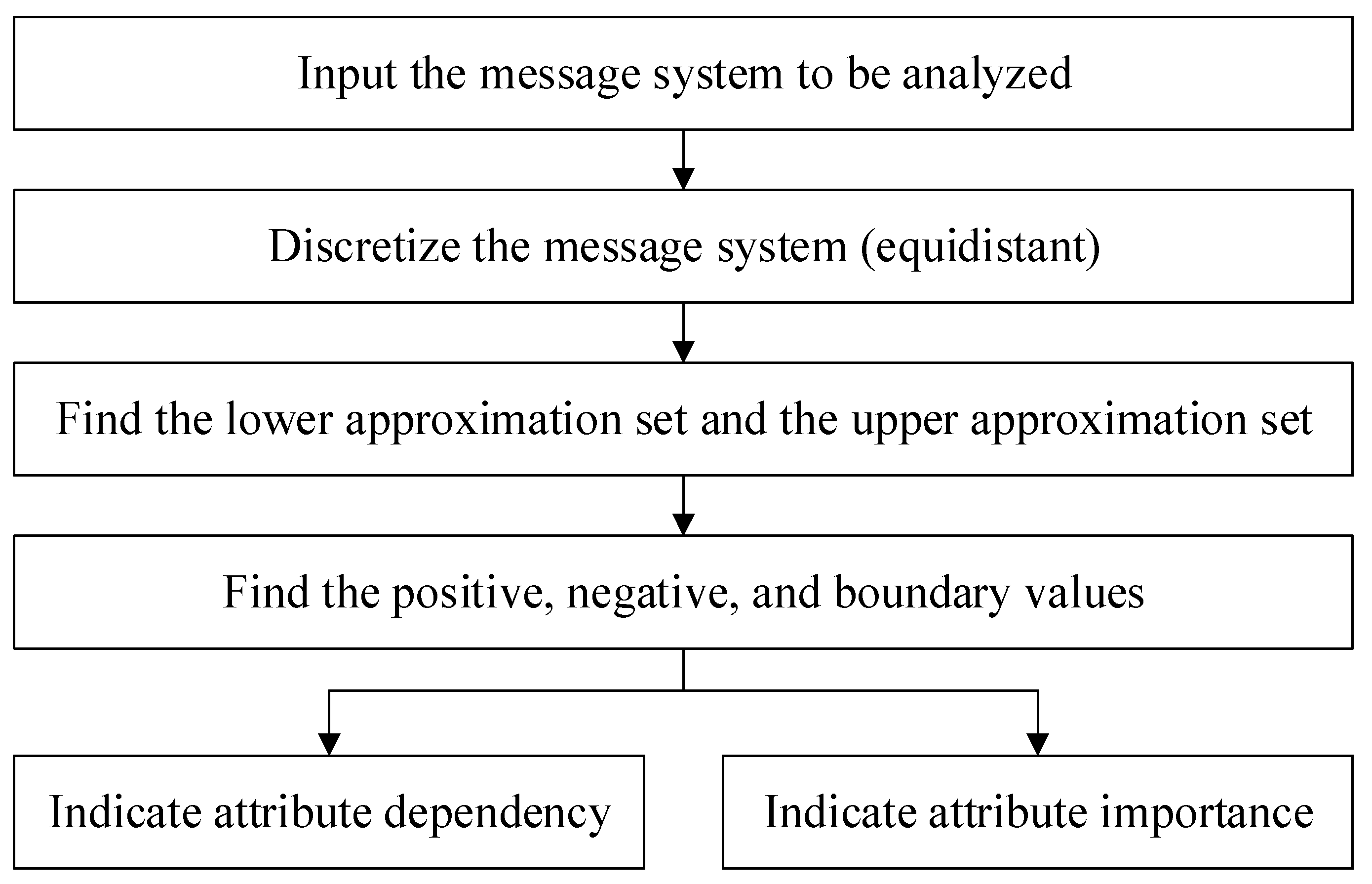
Therefore, we know that γc(D) represents the dependency between decisional attribute D and conditional attribute C. In other words, C can be used to describe the degree of approximation of . Therefore, the importance of the attribute can be measured by the change in value γc(D) when is removed from C. These analytical steps are shown in Figure 2 [25].
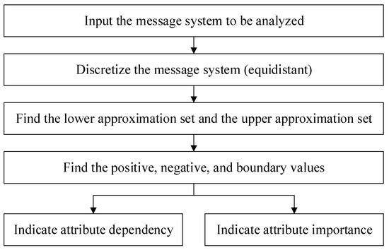
Figure 2.
Block of the analytical steps used in the rough set employed in this study.
2.4. The Grey Relational Grade and Grey Structural Modeling
The grey relational grade plays a crucial role in relational analysis, and its main function is the measurement between two discrete sequences [25,26]. There are two types of model construction: localization grey relational grade (LGRG) and globalization grey relational grade (GGRG) [20,21]. LGRG refers to a given sequence, which can be ranked. In GGRG, the individual sequence can represent the reference sequence, and not only can the sequence be ranked, but also the optimal sequence can be found [25,26,27].
Cluster analysis is the aggregation of similar samples to form clusters. Cluster analysis uses distance as the basis for classification [28,29,30,31,32]. The closer the distance between samples, the higher is their degree of similarity, and they can thus be classified into the same group. Cluster analysis can be divided into hierarchical and non-hierarchical methods. In this study, the proposed matrix arrangement with grey structural modeling (GSM) theory uses the Minkowski distance of the hierarchical method to calculate grey correlation and ranking, thus yielding the cluster status of the overall research results [8,9,32,33,34,35].
Let be the test subject (student) and the test question. The original matrix can then be defined as [28,29,30,31]:
where . Then, apply ranking using the grey correlation, where the range is .
Thus, the LGRG equation is derived as [25,26]:
where is the resolution coefficient, and .
In addition, the GGRG equation can be expressed as [25,26]:
After these calculations of the local and overall grey correlations have been crunched, the GSM structure can be obtained, the ranking of the results can be analyzed, and cluster analysis can be performed to identify the hierarchical relationship of the graphs [32,33,34,35]. The following steps are used to analyze and process the GSM hierarchical structure [25,26,32,33,34,35]:
- (1)
- When represents a hierarchical structure, this hierarchy is composed of a group of structural elements, and the formula is:where and is the class coefficient in which its range is . The matrix formed is as shown below.
For sets and , a multi-level hierarchical set is defined as . Its error value is , with its range defined as and .
- (2)
- Elements in set have mutual homogenous relationships. The principles of formation are described as follows:
- (a)
- For each random , the least number of elements is selected to form the set , , where .
- (b)
- For all , , and .
The hierarchy of GSM structural diagrams is yielded by the clustering of several related elements together using the following equation:
where is a common coefficient with a range of . It can have a common relationship and can be expressed as . Note that can also be formed by the relationship between the upper and lower approximation sets.
3. Analysis of a Practical Example
The participants of the study were 29 freshman students (non-English majors) who had enrolled in a two-semester Freshman English class. The course already included remedial instruction in order to enhance these students’ learning. However, knowing how to increase students’ remedial learning outcomes during limited class time was still a problem. Furthermore, there was no guarantee that students having the same scores actually had the same weaknesses in English. Therefore, in this study, the researcher used rough set theory to discover the dominant attribute influencing students’ final scores. The GSM was then used to cluster students into different groups, and finally customized remedial instruction could be established for each group.
3.1. Calculation of the Attributes Using the Rough Set Theory
Table 1 presents the original data of the study, including the 29 students, and the following five attributes that were influencing students’ final scores:

Table 1.
The original data.
- (1)
- Online discussion board (): students had to finish the assigned writing homework online weekly.
- (2)
- Grammar exercises (): students did the grammar exercises during class time to check their understanding.
- (3)
- Listening exercises (): students did the listening exercises in the textbook during class time.
- (4)
- Vocabulary tests (): students took the NGSL vocabulary quiz at the beginning of the class weekly.
- (5)
- Oral interview (): a structured oral interview was given to each student after the midterm exam.
In addition, the final exam was weighted the same as the mid-term exam, so the arithmetic average of the two scores are used as the scores shown in Table 1.
The calculation steps are described as follows.
- (1)
- Discrete the data into three grades, and they are shown in Table 2
Table 2. The discrete of three grades.
- (2)
- Then, reach condition attributes and decision attributes , the positive posc(D) can be found, and substitute into Equation (11) to obtain the dependent = 0.6207.
- (3)
- Omit the attributes of a1, and by using Equation (12), the significance of σ(a1) = 0.1111.
- (4)
- Then, omit , respectively, the significant of others attribute are:σ(a2) = 0.3333, σ(a3) = 0.1667, σ(a4) = 0.2222 and σ(a5) = 0.0556, respectively.
After defining the attributes, the weighting of each attribute can be calculated through the rough set equation.
3.2. GSM Clustering Generation
To establish the GSM figure, the study first defined the weighting of each attribute. Since the attributes were equally important, the evaluated weighting of each attribute was 100 in this study. Next, the evaluation matrix could be established [25,26].
- (1)
- LGRG calculation
The calculation process is as follows:
- (a)
- Establish the standard sequence.
Through Table 1, the total score is the standard sequence:
x0 = (100, 100, 100, 100, 100, 100, 100)
- (b)
- According to Table 1, each sequence is as shown below:
x1 = (74, 85, 76, 76, 82, 32), x2 = (78, 64, 74, 39, 62, 64), x3 = (92, 88, 85, 66, 53, 89),
x4 = (84, 73, 85, 71, 44, 42), x5 = (60, 64, 79, 48, 45, 72), x6 = (88, 95, 94, 82, 53, 68),
x7 = (86, 91, 91, 40, 62, 79), x8 = (94, 85, 88, 82, 83, 60), x9 = (76, 97, 91, 96, 94, 94),
x10 = (90, 91, 85, 91, 92, 90), x11 = (88, 94, 94, 91, 93, 82), x12 = (68, 74, 66, 84, 89, 51),
x13 = (88, 82, 68, 24, 30, 41), x14 = (88, 85, 88, 78, 84, 95), x15 = (94, 88, 94, 44, 44, 78),
x16 = (90, 97, 86, 87, 90, 73), x17 = (82, 76, 91, 84, 81, 56), x18 = (92, 85, 79, 50, 34, 56),
x19 = (94, 88, 91, 93, 96, 73), x20 = (74, 82, 76, 74, 80, 79), x21 = (88, 82, 91, 57, 71, 57),
x22 = (80, 73, 82, 77, 93, 60), x23 = (78, 82, 88, 29, 38, 83), x24 = (73, 79, 79, 27, 41, 64),
x25 = (86, 94, 88, 69, 57, 96), x26 = (74, 82, 78, 83, 82, 68), x27 = (72, 82, 76, 88, 78, 72),
x28 = (84, 82, 86, 80, 76, 87), x29 = (76, 82, 60, 50, 44, 72)
- (c)
- Calculate the difference sequence.
= (26.0000, 15.0000, 24.0000, 24.0000, 18.0000, 68.0000), = 29.1667
= (22.0000, 36.0000, 26.0000, 61.0000, 38.0000, 36.0000), = 36.5000
= (8.0000, 12.0000, 15.0000, 34.0000, 47.0000, 11.0000), = 21.1667
------------------------------------------------------------------
= (28.0000, 18.0000, 24.0000, 12.0000, 22.0000, 28.0000), = 22.0000
= (16.0000, 18.0000, 14.0000, 20.0000, 24.0000, 13.0000), = 17.5000
= (24.0000, 18.0000, 40.0000, 50.0000, 56.0000, 28.0000), = 36.0000
and Δmax. = 76.0000, Δmin. = 3.0000.
- (d)
- Substitute the data mentioned above into Equation (14), then the LGRG value can be obtained.[0.7171, 0.6897, 0.7779, 0.6945, 0.6780, 0.7819, 0.7369, 0.8154, 0.9059, 0.9142, 0.9126, 0.7408, 0.6217, 0.8720, 0.7176, 0.8707, 0.7879, 0.6820, 0.8851, 0.8004, 0.7515, 0.7853, 0.6747, 0.6573, 0.7972, 0.7995, 0.8003, 0.8414, 0.6896]
- (2)
- GGRG calculation
The calculation process is as follows:
- (a)
- According to Table 1, each sequence is as shown below:
x1 = (74, 85, 76, 76, 82, 32), x2 = (78, 64, 74, 39, 62, 64), x3 = (92, 88, 85, 66, 53, 89),
x4 = (84, 73, 85, 71, 44, 42), x5 = (60, 64, 79, 48, 45, 72), x6 = (88, 95, 94, 82, 53, 68),
x7 = (86, 91, 91, 40, 62, 79), x8 = (94, 85, 88, 82, 83, 60), x9 = (76, 97, 91, 96, 94, 94),
x10 = (90, 91, 85, 91, 92, 90), x11 = (88, 94, 94, 91, 93, 82), x12 = (68, 74, 66, 84, 89, 51),
x13 = (88, 82, 68, 24, 30, 41), x14 = (88, 85, 88, 78, 84, 95), x15 = (94, 88, 94, 44, 44, 78),
x16 = (90, 97, 86, 87, 90, 73), x17 = (82, 76, 91, 84, 81, 56), x18 = (92, 85, 79, 50, 34, 56),
x19 = (94, 88, 91, 93, 96, 73), x20 = (74, 82, 76, 74, 80, 79), x21 = (88, 82, 91, 57, 71, 57),
x22 = (80, 73, 82, 77, 93, 60), x23 = (78, 82, 88, 29, 38, 83), x24 = (73, 79, 79, 27, 41, 64),
x25 = (86, 94, 88, 69, 57, 96), x26 = (74, 82, 78, 83, 82, 68), x27 = (72, 82, 76, 88, 78, 72),
x28 = (84, 82, 86, 80, 76, 87), x29 = (76, 82, 60, 50, 44, 72)
Each sequence can be the standard sequence, and the others are inspected sequences.
- (b)
- Calculate the difference sequences to obtain Δmax. and Δmin.
- (c)
- Calculate the grey relational matrix.The maximum lambda is 16.9732, and corresponding eigenvector are GGRG values: [0.1683, 0.1755, 0.1978, 0.1721, 0.1646, 0.1968, 0.1864, 0.2061, 0.1696, 0.1878, 0.1898, 0.1768, 0.1102, 0.1980, 0.1753, 0.1994, 0.2034, 0.1665, 0.1873, 0.2132, 0.2048, 0.1991, 0.1491, 0.1503, 0.1923, 0.2122, 0.2073, 0.2120, 0.1733]
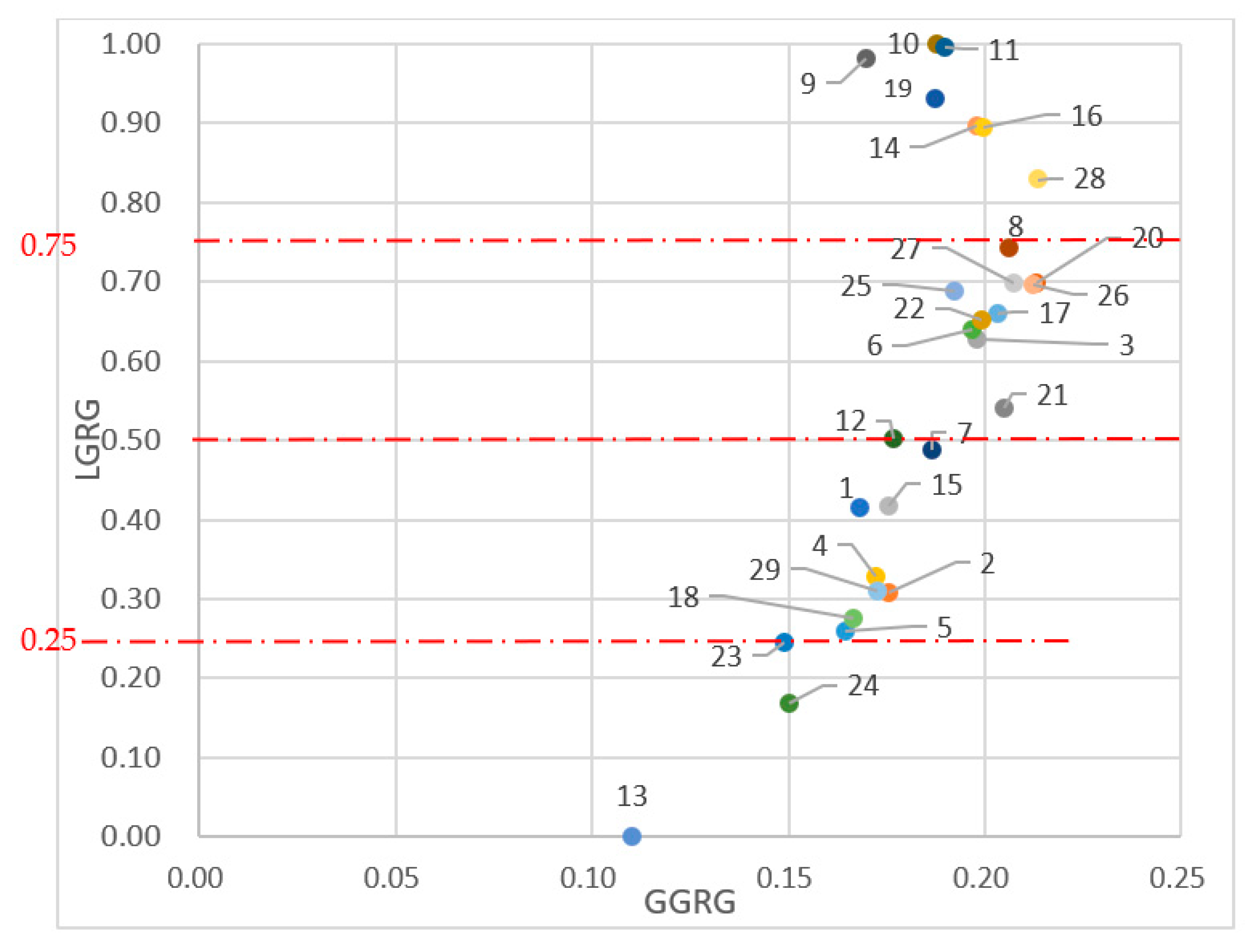
After the whole calculation, the whole answer can be calculated. Based on the GGRG and LGRG values of the students, the GSM figure can be generated, which is shown in Figure 3. Due to there being only 29 students in this study, the researcher decided to divide them into only four groups.
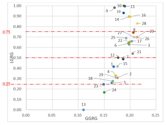
Figure 3.
GSM student clustering.
4. Results and Discussion
The weighting of the five attributes are shown in Table 3.
Table 3.
The weighting of the attributes.
The attributes were then sorted from the most to the least weighty: . According to rough set theory, this means the attribute having the largest impact on students’ final scores was (grammar exercises), and the attribute having the smallest impact on students’ final scores was (oral interview). Therefore, a teacher of this course wanting to enhance students’ performance in English should spend more time teaching or reviewing grammar exercises. The study also revealed that the attribute influencing students’ final scores second most was (vocabulary tests). Whereas grammar is the learning of word forms (morphology) and sentence structure (syntax), vocabulary learning refers to the usage of word order in a particular field with a specific purpose. Thus, it is suggested that the teacher adjust the curriculum design by adding more grammar and vocabulary tasks in class. For example, teachers can design tasks such as multiple choice, true/false, or chronological sequencing (putting a short story into the correct order). In this way, students would not only learn the rules, but they could also improve their language communication. In addition, students would understand their weaknesses in English and through targeted remedial instruction, have a better chance at obtaining higher scores in the second semester. Moreover, students would be learning with a variety of grammar and vocabulary tasks provided by the teacher. These tasks should be well scaffolded; that is, they need to be more controlled, and less cognitive. Gradually, these ways of learning should become habits among the students; even after class, these students will still know “how to learn” on their own.
Once the teacher knew the key points that the students needed to strengthen, another issue needing attention was how to ensure the students learn these key points in the classroom effectively. Ideally, each student would need to focus on strengthening his or her weakest area. In this study, the GSM was used to cluster students (see Figure 3). In Figure 3, the vertical axis is the LGRG value; the horizontal axis is GGRG value. The 29 red dots on the graph represent the 29 students in this study. The value of LGRG ranges from 0 to 1, meaning that the value of the teacher’s expectation of student achievement is up to 100, which is 1 on the graph. The value of GGRG represents the actual performance of each student. If the students (the dots) were closer to each other, it would mean that their actual performance was similar. Due to there being only 29 students in this study, the researcher divided the value of LGRG into four equal categories, as shown in Table 4.
Table 4.
Clustering students into groups.
It would be easier for the teacher to provide appropriate remedial instruction to each group shown in Table 4 individually. The students, grouped with other students of the same level, would be able to support one another. The teacher would need only to prepare four remedial instruction packages, one for each of the four groups, thus lowering his or her workload. When the groups are working on the assigned grammar and vocabulary tasks, the teacher can circulate and participate in group discussions. Due to the students in the group struggling with the same point at the same level, the teacher can effectively explain the key points in detail to each group. In the process of doing so, the teacher can trace student performance and shift students to other groups as they gain mastery.
In Figure 3, although there were only three students in Group 4 (the lowest level), the distance between Student No. 23 and Student No. 24 is close whereas Student No. 13 is far below them. Based on GGRG, this shows that the real ability of No. 23 and No. 24 was similar; however, the ability of No. 13 was lagging far behind the other two students. When the teacher gave remedial instruction, he or she would need to pay more attention to Student No. 13. Figure 3 also shows that Group 1 has the best English proficiency with the LGRG value ranging from 0.75–1. In Group 1, Student No. 10, having the best performance, is at the top of the graph. Therefore, the teacher should give Group 1 more challenging grammar and vocabulary tasks. In Table 3, the researcher noticed one thing, that is, the majority of the students belonged to Group 2 and Group 3. Hence, when designing the curriculum, the content should be moderately difficult. Therefore, most of the students in the class should be able to absorb the information. Gradually, they can improve their English ability and may have the opportunity to shift to higher levels.
5. Conclusions and Implications
The major findings of this study, which integrated rough set theory and GSM to establish remedial instruction for students in an effective way, are:
- (1)
- Using rough set theory and GSM, a teacher can calculate the weighting of attributes and identify students’ learning problems. This insight allows him or her to adjust the curriculum design and teaching strategies to fit students’ needs. Before final grades are sealed at the end of the semester, students can follow their teacher’s remedial instruction to strengthen their weak points and achieve higher scores at the end of semester.
- (2)
- In previous studies, determining who needs remedial instruction has basically been based on whether a student passes or fails the subject. Students who had scored below 60 would be asked to take the remedial instruction class. Usually, the remedial class would be offered after school, and the teacher would ask the students to do many exercises. The problem with that approach is that the students would have to do exercises in every section instead of just doing the section that they really did not understand. Basically, it is a waste of time. However, through GSM, a teacher can easily cluster students who are all struggling with the same point at the same level. Then the teacher can provide customized remedial instruction to each group in class. Due to them being low-level students, it is very important for the teacher to guide them in “how to learn.” Besides, letting them learn with their peers is also crucial to their learning experience.
- (3)
- In this study, GSM objectively presents the distribution of students’ actual English performance. With LGRG showing the teacher’s expectation score on the vertical axis and GGRG showing the students’ actual performance on the horizontal axis. The results can conveniently be presented visually.
- (4)
- Together, the rough set and GSM can analyze small samples objectively. With only 29 students in the example analyzed in this study, it would have been difficult to find objective research tools to cluster such small samples. However, due to the characteristics of grey theory, small samples can be analyzed easily.
A limitation of this study is that there were only five attributes affecting the final scores. In future research, using more attributes should result in the ability to provide more precise remedial instruction for students. In the discretization of rough set, this study chose to use three grades because the data resolution of four grades and five grades is not enough. In addition, the implications for future research include doing research in different fields, and applying other soft methods, such as fuzzy theory, of analyzing small samples to find the best solution. Moreover, the computer toolbox of rough set and GSM, which is convenient for users to download and use in various fields for clustering, will be developed in the future.
Funding
The research was funded by MOE grant number PED1080111.
Institutional Review Board Statement
Not applicable.
Informed Consent Statement
Not applicable.
Conflicts of Interest
The author declares no conflict of interest.
References
- Tai, J.; Ajjawi, R.; Boud, D.; Dawson, P.; Panadero, E. Developing evaluative judgement: Enabling students to make decisions about the quality of work. High. Educ. 2017, 76, 467–481. [Google Scholar] [CrossRef] [Green Version]
- Schrader, D.E.; Erwin, T.D. Assessing Student Learning and Development: A Guide to the Principles, Goals, and Methods of Determining College Outcomes. J. High. Educ. 1992, 63, 463. [Google Scholar] [CrossRef]
- Hatti, J.; Timperley, H. The power of feedback. Rev. Educ. Res. 2007, 77, 81–112. [Google Scholar] [CrossRef]
- Jiang, S.; Wang, C.; Weiss, D.J. Sample Size Requirements for Estimation of Item Parameters in the Multidimensional Graded Response Model. Front. Psychol. 2016, 7, 109. [Google Scholar] [CrossRef] [PubMed] [Green Version]
- Liu, S.; Forrest, J. The current developing status on grey system theory. J. Grey Syst. 2007, 2, 111–123. [Google Scholar]
- Deng, J.L. Grey control system. J. Huazhong Univ. Sci. Technol. 1982, 3, 9–18. [Google Scholar]
- Deng, J.L. Theory of Grey System; Huazhong University of Science and Technology Press: Wuhan, China, 1990. [Google Scholar]
- Masatake, N.; Chen, T.L.; Tsai, C.P.; Chiang, H.J.; Sheu, T.W. Rough structural modeling and its application. In Proceedings of the 2013 International Conference on Grey System Theory and Kansei Engineering Conferences, Taichung, Taiwan, 30 November–2 December 2013; pp. 113–122. [Google Scholar]
- Yamaguchi, D.; Li, G.D.; Masatake, N. Verification of effectiveness for grey relational analysis models. J. Grey Syst. 2007, 10, 169–181. [Google Scholar]
- Pawlak, Z. Rough Sets. Int. J. Comput. Inf. Sci. 1982, 11, 341–356. [Google Scholar] [CrossRef]
- Pawlak, Z. Rough set theory and its applications. J. Telecommun. Inf. Technol. 2002, 3, 7–10. [Google Scholar]
- Dai, S. Rough Approximation Operators on a Complete Orthomodular Lattice. Axioms 2021, 10, 164. [Google Scholar] [CrossRef]
- Sokal, R.R.; Sneath, P.H.A. Principals of Numerical Taxonomy; W.H. Freeman: San Francisco, CA, USA, 1963. [Google Scholar]
- Fonseca, J.R. Clustering in the field of social sciences: That is your choice. Int. J. Soc. Res. Methodol. 2012, 16, 403–428. [Google Scholar] [CrossRef]
- Rai, P.; Singh, S. A survey of cluster techniques. Int. J. Comput. Appl. 2010, 7, 1–5. [Google Scholar]
- Xu, D.; Tian, Y. A Comprehensive Survey of Clustering Algorithms. Ann. Data Sci. 2015, 2, 165–193. [Google Scholar] [CrossRef] [Green Version]
- Kaufman, L.; Rousseeuw, P.J. Finding Groups in Data: An Introduction to Cluster Analysis; Wiley-Interscience: Hoboken, NJ, USA, 1990. [Google Scholar]
- Hassanien, A.E.; Ali, J.M. Rough Set Approach for Generation of Classification Rules of Breast Cancer Data. Informatica 2004, 15, 23–38. [Google Scholar] [CrossRef]
- Tabakov, M.; Chlopowiec, A.; Chlopowiec, A.; Dlubak, A. Classification with Fuzzification Optimization Combining Fuzzy Information Systems and Type-2 Fuzzy Inference. Appl. Sci. 2021, 11, 3484. [Google Scholar] [CrossRef]
- Wu, W.; Mi, J.; Zhang, W. Generalized fuzzy rough sets. Inf. Sci. 2003, 151, 263–282. [Google Scholar] [CrossRef]
- Yeung, D.; Chen, D.; Tsang, E.; Lee, J.; Xizhao, W. On the generalization of fuzzy rough sets. IEEE Trans. Fuzzy Syst. 2005, 13, 343–361. [Google Scholar] [CrossRef]
- You, M.L.; Wei, M.C.; Fang, W.H.; Wen, K.L. Study on the student test score weighting by integrating grey relational grade and rough set. J. Grey Syst. 2013, 16, 113–120. [Google Scholar]
- Wen, K.L.; Lee, Y.T. Applying rough set theory in the function group analysis for phenolic amide compounds. Comput. Electr. Eng. 2012, 38, 11–18. [Google Scholar] [CrossRef]
- Wen, K.-L.; Changchien, S.-K. The Weighting Analysis of Influence Factors in Gas Breakdown via Rough Set and GM(h,N). J. Comput. 2008, 3, 17–24. [Google Scholar] [CrossRef]
- Wang, B.T.; Wang, J.R.; Wen, K.L.; Masatake, N.; Liang, J.C. Kansei Engineering Fundamentals; Taiwan Kansei Information Association: Taichung, Taiwan, 2011. [Google Scholar]
- Nguyen, P.T.; Nguyen, P.H.; Pham, D.H.; Tsai, C.P.; Masatake, N. The proposal for application of several grey methods in evaluating and improving the academic achievement of students. J. Taiwan Kansei Inf. 2013, 4, 179–190. [Google Scholar]
- Stanujkíc, D.; Karabaševíc, D.; Popovíc, G.; Stanimirovíc, P.S.; Smarandache, F.; Sarӑcevíc, M.; Ulutąs, A.; Katsikis, V.N. An innovative grey approach for group multi-criteria decision analysis based on the median of ratings by using python. Axioms 2021, 10, 124. [Google Scholar] [CrossRef]
- Silva, E.C.; Correia, A.; Borges, A. Unveiling the Dynamics of the European Entrepreneurial Framework Conditions over the Last Two Decades: A Cluster Analysis. Axioms 2021, 10, 149. [Google Scholar] [CrossRef]
- Biswas, S.; Pamucar, D. Facility Location Selection for B-Schools in Indian Context: A Multi-Criteria Group Decision Based Analysis. Axioms 2020, 9, 77. [Google Scholar] [CrossRef]
- Trebuňa, P.; Halčinová, J. Mathematical Tools of Cluster Analysis. Appl. Math. 2013, 4, 814–816. [Google Scholar] [CrossRef] [Green Version]
- Battaglia, O.R.; Di Paola, B.; Fazio, C. A New Approach to Investigate Students’ Behavior by Using Cluster Analysis as an Unsupervised Methodology in the Field of Education. Appl. Math. 2016, 7, 1649–1673. [Google Scholar] [CrossRef] [Green Version]
- Wang, B.T.; Sheu, T.W.; Liang, J.C.; Tzeng, J.W.; Masatake, N. Clustering the English reading performances by using GSP and GSM. J. Grey Syst. 2012, 15, 87–93. [Google Scholar]
- Wang, B.T.; Chen, H.T.; Chang, H.Y. Using GRA and GSM methods to identify the learning strategies of good language learners. Int. J. e-Educ. e-Bus. e-Manag. e-Learn. 2013, 3, 397–401. [Google Scholar] [CrossRef]
- Wang, B.T.; Sheu, T.W.; Liang, J.C.; Tzeng, J.W.; Masatake, N. The integrated methods of GSP and GSM in concept diagnosis for English grammar. J. Taiwan Kansei Inf. 2011, 2, 87–100. [Google Scholar]
- Sheu, P.H. Applying Student-Problem Chart, Grey Student-Problem Chart and Grey Structure Modeling to Analyze the Effect of an Elementary School English Remedial Instruction. Int. J. Engl. Linguist. 2019, 9, 49. [Google Scholar] [CrossRef]
Publisher’s Note: MDPI stays neutral with regard to jurisdictional claims in published maps and institutional affiliations. |
© 2021 by the author. Licensee MDPI, Basel, Switzerland. This article is an open access article distributed under the terms and conditions of the Creative Commons Attribution (CC BY) license (https://creativecommons.org/licenses/by/4.0/).