Article

Advanced Proportional-Integral-Derivative Control Compensation Based on a Grey Estimated Model in Dynamic Balance of Single-Wheeled Robot

1
College of Information and Mechanical & Electrical Engineering, Ningde Normal University, Ningde 352100, China
2
Department of Mechanical Engineering, National Chin-Yi University of Technology, Taichung 41170, Taiwan
3
Transway Plastic Co., Ltd., Taichung 41280, Taiwan
4
Department of Mechanical Engineering, National Cheng Kung University, Tainan 70101, Taiwan
*
Author to whom correspondence should be addressed.
Axioms 2021, 10(4), 326; https://doi.org/10.3390/axioms10040326
Submission received: 24 September 2021 / Revised: 19 November 2021 / Accepted: 25 November 2021 / Published: 30 November 2021
(This article belongs to the Special Issue Grey System Theory and Applications in Mathematics)

Abstract

:
This paper aims to design a one-wheeled robot as regards its pitch freedom and balance control on the one hand and to assess the application feasibility of the GM (1,1) swing estimation controller on the other. System control focuses mainly on one-wheeled robot stability, body swings in position, and speed control. Mathematical modeling and GM (1,1) prediction control are under investigation. The mathematical modeling is firstly conducted through referencing to the Newtonian mechanics and the Lagrange equation, from which the robot transfer function and state-space differential equation are derived. Next, the linear quadratic regulator is applied as the control rule at the balance point. Applying GM (1,1) to assess the robot gyro signal at a dynamic state is a discussion. Next, model reference estimation control is processed, and a mathematical model of the balance control method is completed. Finally, a simulation is conducted to verify the feasibility of the GM (1,1) estimation reference model. The linear quadratic regulator, which is credited with tenacity, can provide pitch swing and balance control of the one-wheeled robot.

1. Introduction

A one-wheeled robot is a system that is dynamically stable yet statically unstable. It is regarded as a completely new robot concept. One-wheeled robots have become a research focus among international scholars. They are characterized by insensitiveness to external interference, high maneuverability, and low rolling friction. They can stand up from the ground phase with ease. Their swing phase of walking is quite similar to the inverted pendulum. One-wheeled robots are typically mobile devices for studying control theory. With low cost and simple structure, their physical parameters are easy to adjust. An unstable system is characterized by a higher order, instability, multiple variables, nonlinearity and robust coupling. One-wheeled robots can effectively reflect key problems during the control process, including stability, swing position walking speed, tracking, etc. They can also be used to examine different theories of control. Therefore, the potential application and market prospects of one-wheeled robots are enormous. One-wheeled robots can, indeed, generate tremendous economic benefits.
There has, over the past few years, been a lot of research dealing with one-wheeled robots. In 1997, scholars from Carnegie Melon University and Hong Kong University conducted research on “gyro stability” one-wheeled robots [1,2]. The intelligence lab of the University of Tsukuba proposed a new one-wheeled robot design based on the principle of an inverted pendulum. This design controlled the wheel’s forward and backward movement and acceleration to maintain the balance control of the robot’s pitch freedom and straight walking. This design also controlled the left–right direction and the center of gravity’s movement. The body tilted left and right, thus enabling the robot to turn [3,4]. In 2005, Carnegie Melon University and Hong Kong University designed, on the basis of the principle of an inverted pendulum, a system controlling robot state balance in two vertical directions [5,6]. In 2006, the University of California, utilizing a gyroscope and acceleration meter, collected robot state signals. “Unibot”, an entirely new robot, could walk with small-angle oscillation while maintaining body stability [7]. So far, various inverted pendulum systems have been established, applying traditional control theory and modern control theory.
The control methods of the inverted pendulum can be categorized into three types, namely linear control methods [8,9,10,11,12,13,14], prediction control and structure-changing control methods [13,15], and intelligence control [16,17,18,19].
Linear control method: The system conducts quasi-linear processing of the nonlinear model of the inverted pendulum system to obtain a linearized model around the stable point. Various linear system controllers are used to attain an expected controller [8,9,10]. For example, in 1976, Mori linearized the inverted pendulum near the stable point, then applied mind space to design a proportional differential controller. In 1980, Furuta completed second-order inverted pendulum control based on linearization. In 1984, Furuta first succeeded in dual motor third-order inverted pendulum physical object control. Wattes (1984) used a linear quadratic regulator to control the inverted pendulum. This method caused a slight linearization error. In addition, this simple model is easy to control. It could solve stability control problems with an inverted pendulum [11,12,13,14].
Prediction control and structure-changing control method: Linear control theory and the inverted pendulum system are multi-variable and nonlinear. Therefore, studying them in terms of prediction control, structure-changing control, and self-adjustment control is necessary. As a method of optimization, prediction control has a greater emphasis on model function than on structure. Structure-changing control is nonlinear. It can control an object by pulling it from any location to the gliding curve while maintaining stability and tenacity. The system, however, may continue to shake. Such a method, theoretically, has a better control effect. However, control complexity and high cost cannot instantly be applied to a fast-changing system. This is the main point facing prediction control [13,15].
Intelligence control: Intelligence control methods, including mainly nerve control, fuzzy control, and simulation intelligence control, have been applied to the inverted pendulum system [16,17,18,19]. Nerve control is characterized by self-adjustment, parallel processing, high tenacity, faster speed, and adjustment. However, nerve control lacks a dynamic nerve net for controlling problems appropriately. In addition, the number of multi-layer nets, the number of hidden neurons, and the selection of activation functions are short of a guiding principle. The fuzzy control system requires a large knowledge database and a corresponding inference mechanism. Such a control method, therefore, cannot meet the needs of instant control.
Economic prosperity has led to more and more vehicles entering our daily life. Cars are a fast, convenient, and time-saving means of transportation. A variety of personalized cars have been designed to satisfy different needs. Cars, however, can cause air pollution and noise. Car production requires complex technology. With traffic jams, safety, and parking problems becoming serious, car driving is getting less and less efficient.
In contrast, one-wheeled robots are, without a doubt, an economical and practical means of transportation. Indeed, one-wheeled robots are free from geographical restrictions. They can move around with ease. They are used for rescue, transportation, and mineral surveys. Indeed, they can generate tremendous economic value. Therefore, this paper aims at mathematical modeling of the one-wheeled robot [13,15]. The GM (1,1) prediction algorithm is employed to implement control, complete body motion stability, and self-balance [20,21].
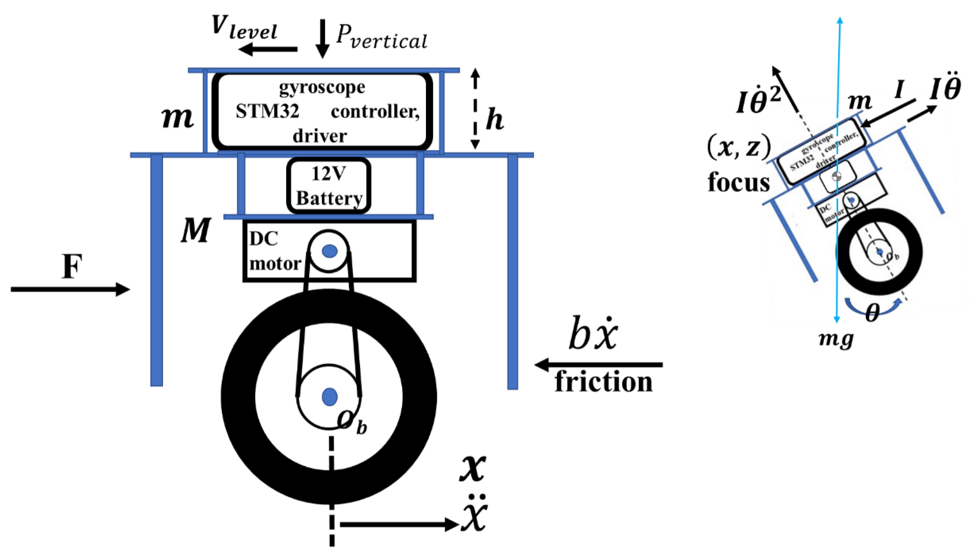
Meanwhile, it also takes into consideration the quickness and stability of the system response. This study shows that grey GM (1,1) prediction applies to robot mathematical modeling. Overall, the single-wheel robot motion system in this study is shown in Figure 1.
According to the mathematical model of the single-wheeled robot, it belongs to a kind of inverted pendulum robot with a single contact point. This robot is typically a statically indeterminate system because its force balance is based on a single contact point. Once it achieves dynamical balance, including pitch and roll stability, the robot requires a complex process to drive the wheel mechanism to provide pitch and roll stability. Generally, there are two methods for providing these two kinds of stability. One is controlling accelerating or decelerating to obtain the torque of the robot to provide the dynamical balance by using the robot’s inertia [1,2,3,4,22]. The other uses an external centrifugal force to maintain stability, such as a spinning flywheel [23,24,25,26]. However, these two methods are both based on inertia control systems. Their stability ability still depends on self-torque or external centrifugal force, which makes the process of stability complex and challenging.
Generally, studies about the balance of the single-wheel robot are based on the proportional–integral–derivative (PID) controller, because of the advantages provided by the PID control method [1,9,27,28,29]. The PID control mothed is feasible to implement quickly into an embedded system. Moreover, the PID control method can also precisely estimate the system response according to its gain [30]. This gain can track errors and treat the system even when the control parameters are unknown. Overall, the PID control method is based on feedback to control the system using integral and derivative relations between input and output signals.
The performance of the PID control method is related to all three gains, which impact transient responses such as settling time, overshoots, oscillations. In other words, while the state space cannot be estimated, the PID gains struggle to resist the uncertainties and disturbances. However, the PID control method cannot provide optimal control or stability for the system. In addition, the common problem of PID control is that the system experiences an excessive delay or uncertainty, which leads the system to respond without enough time [30]. Thus, this study develops the single-wheeled robot’s balance control by using PID combined with GM (1,1). The GM (1,1) can estimate the dynamic state-space of motion on the single-wheel robot, compensating for the time delay effect rapidly from PID control.
This study aims to design a one-wheeled robot as regards its pitch freedom and balance control on the one hand and to assess the application feasibility of the GM (1,1) swing estimation controller on the other. System control focuses mainly on one-wheeled robot stability, body swings in position, and speed control, which provide dynamical balance by using the robot’s inertia.
According to the balance principle of the single-wheeled robot (Figure 2), GM (1,1), through the relation between inclination angle and wheel rotation velocity, is used to estimate the gyroscope signal when the robot is dynamic. Finally, GM (1,1) is verified by simulation—the feasibility of the reference model and controlling the robot wheel’s acceleration to eliminate the robot’s inclination is estimated. Thus, the robot can balance as soon as possible under any conditions.
This paper organizes the study as follows: Section 2 describes the mathematical model of the one-wheeled robot. Section 3 describes the concept of the grey prediction model. Section 4 verifies the effectiveness of GM (1,1) combined with PID control for the dynamic balance of the one-wheeled robot system. Section 5 provides the discussions and conclusions of this study.

2. Mathematical Model of the One-Wheeled Robot

This section deals with the mathematical model in relation to the robot.

2.1. Analysis of Robot Load-Carrying Capability

The single-wheel robot system force analysis diagram is shown in Figure 2. The symbols of the balance algorithms are shown in Table 1. The control system was established by using the proportional differential negative ratio to control the wheel rotation velocity and then feedback the velocity to adjust the situation of the robot. According to the control system, the control process was a closed-loop to maintain the robot’s stability.
According to Newton’s laws of motion, an external force produces an angular acceleration x(t) of the single-wheel car. While the single wheel robot becomes stable, the force along the direction perpendicular to the ground can be estimated by the model inclination angle and the acceleration of the wheel movement [15,17,18].

2.2. Equation of Robot System Dynamics

First, the following dynamic equation is obtained by adding hand thrust and the force in the horizontal direction of the robot [10,11].
M x ¨   +   b x ˙ + V level   = F
The body equation of robot horizontal direction is
V level   = m x ¨ + mh θ ¨ cos θ     mh θ ˙ 2 sin θ
Substituting Equation (2) into Equation (1), we can obtain the motion equation
( M + m ) x ¨ + b x   ˙ + mh θ ¨ cos θ   mh θ ˙ 2 sin θ = F
The combined horizontal and vertical force [8,17] is
P vertical sin θ + V level cos θ     mgsin θ = mh θ ¨ + m x ¨ cos θ
Dividing Equation (4) by the vertical and horizontal force, we can obtain equation of body barycenter torque
P vertical Isin θ     V level Icos θ = I θ ¨
Additionally, combining Equation (4) with Equation (5), the dynamic equation is
( I + mh 2 ) θ ¨ + mghsin θ = mh x ¨ cos θ
( M + m ) x ¨ + b x   ˙   mh θ ¨ = u i
After system linearization, we proceed with the Laplace transform to generate the system equation:
( I + mh ) θ ( s ) s 2   mgh θ ( s ) = mhX ( s ) s 2
( M + m ) X ( s ) s 2 + bX ( s )   mh θ ( s ) s 2 = U i ( s )
Assuming the initial condition is 0, the transfer function is calculated, and we can obtain the relation between X ( s ) and pendulum angle θ .
X ( s ) = [ ( I + mh 2 ) mh g s 2 ] θ ( s )
Additionally, substituting Equation (10) into Equation (9), we can obtain the linearized dynamic equation of the robot in the straight-up-stable state:
( M + m ) [ ( I + mh 2 ) mh + g s ] θ ( s ) s 2 + b [ ( I + mh 2 ) mh + g s ] θ ( s ) s     mh θ ( s ) s 2 = U i ( s )
thus,
θ ( s ) U i ( s ) = mh [ ( M   +   m ) ( I   +   mh 2 )     ( mh ) 2 ] s 2 s 4   +   b ( I   +   mh 2 ) [ ( M   +   m ) ( I   +   mh 2 )     ( mh ) 2 ] s 3 ( M   +   m ) mgh   [ ( M   +   m ) ( I   +   mh 2 )     ( mh ) 2 ] s 2 bmgh [ ( M   +   m ) ( I   +   mh 2 )     ( mh ) 2 ] s
Additionally, the linearized state-space motion equation of Equation (12) becomes Equations (13) and (14).
[ x ˙ x ¨ θ ˙ θ ¨ ] = [ 0 1 0     ( I   +   mh 2 ) b I ( M   +   m )   +   Mmh 2 0 0 m 2 gh 2 I ( M   +   m )   +   Mmh 2 0 0 0 0     mhb I ( M   +   m )   +   Mmh 2 0 1 mgh ( M   +   m ) I ( M   +   m )   +   Mmh 2 0 ] [ x x ˙ θ θ ˙ ]   +   [ 0 I   +   mh 2 I ( M   +   m )   +   Mmh 2 0 mh I ( M   +   m )   +   Mmh 2 ] u i
y = [ 1 0 0 0 0 0 1 0 ] [ x x ˙ θ θ ˙ ] + [ 0 0 ] u i

3. Grey Prediction Model

In grey system theory, the prediction of the system of non-deterministic information is called the grey prediction model, which is explained as follows. Professor Deng Julong proposed the grey system theory in 1981. It is a method of predicting systems with uncertain factors. By identifying system factors and generating and processing the original data, it searches for changes in the system and generates regular data sequences. Then, it establishes the corresponding differential equation model to predict the future development trend and future state of things [19,21,31,32].

3.1. The Establishment of the GM (1,1) Model

Assuming that the time series X ( 0 ) has an observation value X ( 0 ) = { x ( 0 ) ( 1 ) , x ( 0 ) ( 2 ) , , x ( 0 ) ( n ) } , in order to be able to become regular time series data, a first accumulate generation operation [21,32,33] is performed, and to obtain
X ( 1 ) ( t ) = n = 1 t X ( 0 ) ( n )
and to attain the newly generated sequence X ( 1 ) , X ( 1 ) = { x ( 1 ) ( 1 ) , x ( 1 ) ( 2 ) , , x ( 1 ) ( n ) } . The newly generated sequence X ( 1 ) obeys the exponential law, then the generated differential
dx dt + ax = u
Equation (16) indicates that the variable is continuous with respect to the first-order differential equation of time. Therefore, by solving the differential equation of Equation (16), we can obtain
x ( t ) = ce a ( t 1 ) + u a
When t = 1 , x ( t ) = x ( 1 ) , and c = x ( 1 ) u a , according to Equation (17), it can obtain the discrete form differential equation, as shown in Equation (18).
x ( t ) = ( x ( 1 ) u a ) e a ( t 1 ) + u a
where
  • x is the background value of dx dt , also called the initial value.
  • a and u are the grey parameters to be calculated, where a is the development coefficient, reflecting the development trend of x
  • u is the grey effect value, which reflects the changing relationship among the data.
According to the definition of the whiteness derivative, dx dt is generated by first accumulating, so Equation (18) can be rewritten as
dx dt = x ( 1 ) ( t + 1 )   x ( 1 ) ( t )
when t is small enough, there will be no abrupt change in the variable x from x ( t ) to x ( t + t ) ; hence, the average of x ( t ) and x ( t + t ) is taken as the background value, and shown in Equation (20)
x ( 1 ) = 1 2 [ x ( 1 ) ( t ) + x ( 1 ) ( t + 1 ) ]
Equation (20) is substituted into Equation (19) to obtain
x ( 0 ) ( t + 1 ) = 1 2 a [ x ( 1 ) ( t )   +   x ( 1 ) ( t + 1 ) ] + u
Based on Equation (21), thus
[ x ( 0 ) ( 2 ) x ( 0 ) ( 3 ) x ( 0 ) ( n ) ] = a [ 1 2 ( x ( 1 ) ( 1 )   +   x ( 1 ) ( 2 ) ) 1 2 ( x ( 1 ) ( 2 )   +   x ( 1 ) ( 3 ) ) 1 2 ( x ( 1 ) ( n - 1 )   +   x ( 1 ) ( n ) ) ] + u
Organizing Equation (22) by using the new assuming parameter,
{ Y = [ x ( 0 ) ( 2 ) x ( 0 ) ( 3 ) x ( 0 ) ( n ) ] T B = [ 1 2 ( x ( 1 ) ( 1 )   +   x ( 1 ) ( 2 ) ) 1 2 ( x ( 1 ) ( n - 1 ) + x ( 1 ) ( n ) ) ] α = ( a u ) T
where Y is the data vector, B is the data matrix, and α is the parameter vector.
Equation (22) can reduce into
Y = B α
Using the least square method in α ^ = ( a u ) T = ( B T B ) 1 B T Y , we can obtain these values and then substitute them into the differential equation,
x ^ ( 1 ) ( t ) = ( x ( 1 ) u a ) e a ( t     1 ) + u a
Equation (25) is the time response function of the GM (1,1) model, and to inverse accumulate it into the x ^ ( 1 ) ( t ) sequence, and to achieve the prediction of x ^ ( 0 ) ( t ) ,
x ^ ( 0 ) ( t ) =   x ^ ( 1 ) ( t ) x ^ ( 1 ) ( t     1 ) = ( x ( 0 ) ( 1 ) u a ) ( 1     e a ) e a ( t     1 )
Hence, Equation (26) is the calculated form of the GM (1,1) prediction model. To sum up, the GM (1,1) modeling steps are as follows:
  • Calculating an accumulation sequence x ( 1 ) from the original data sequence x ( 0 ) ;
  • Establishing a data vector, Y, and a data matrix, B;
  • Calculating the inverse matrix ( B T B ) 1 for the least square method;
  • Estimating a ^ and x ^ , according to U ^ = ( B T B ) 1 B T Y
  • Calculating the fitting value x ^ ( 1 ) ( t ) with the time response equation, and then restoring it with the post subtraction operation, that is: x ^ ( 0 ) ( i ) = x ^ ( 1 ) ( i ) x ^ ( 1 ) ( i 1 )   ( i = 2 , 3 , 4 , , N )
  • Following the accuracy test, prediction is corrected until the error becomes minimal.

3.2. The Checking of GM (1,1) and Residual

The GM (1,1) model [21,32,33] includes three forms: residual checking, correlation checking, and posterior error checking. When the GM (1,1) model established by the original data sequence is not accurate enough, the GM (1,1) residual model is used to modify and improve the accuracy. In the established GM (1,1) model of x ( 0 ) , the predicted value of the generated sequence is obtained, and the residual sequence is defined as e ( 0 ) ( k ) = x ( 1 ) ( k ) x ^ ( 1 ) ( k ) . If k = t, t + 1, t + 2…, n, then the corresponding residual sequence is
e ( 0 ) ( k ) = [ e ( 0 ) ( 1 ) e ( 0 ) ( n ) ]
We calculate the generating sequence e ( 0 ) ( k ) in Equation (27), and build up the corresponding GM (1,1) model as Equation (28).
e ^ ( 1 ) ( t + 1 ) = ( e ( 0 ) ( 1 ) u e a e ) e a e k + u e a e
Then, we can obtain the modified model, as shown in Equation (29)
x ( 1 ) ( t + 1 ) = ( x ( 0 ) ( 1 ) u a ) e - ak + u a + δ ( k t ) ( a e ) ( e ( 0 ) ( 1 ) u e a e ) e - a e k
where δ ( k t ) { 1 k t 0 k t is the modified parameters.
Overall, the checking steps of GM (1,1) and residual are as follows:
  • Residual test, calculated separately:
    Residual: E ( k ) = x ( 0 ) ( k ) x ^ ( 0 ) ( k ) ,   k = 2 , 3 , , N ;
    Relative residual: e ( k ) = [ x ( 0 ) ( k ) x ^ ( 0 ) ( k ) ] x ( 0 ) ( k ) ,   k = 2 , 3 , , N .
  • A posteriori error test, calculated separately:
    x ( 0 ) mean value: X ¯ = 1 N k = 1 N x ( 0 ) ( k ) ;
    x ( 0 ) variance: S 1 = 1 N k = 1 N ( x ( 0 ) ( k ) x ¯ ) 2 ;
    Mean value of residuals: E ¯ = 1 N 1 k = 2 N E ( k ) ;
    The variance of residuals: S 2 = 1 N k = 2 N ( E ( k ) E ¯ ) 2 ;
    Posterior error ratio: C = S 2 S 1 ;
    Small error probability: S 2 = Probe { | E ( k ) E ¯ | < 0.6745 S 1 } .
  • The comparison table of prediction accuracy grades is shown in Table 2.

4. Simulation and Verification

This paper employs an STM32 controller and a 12 V Servomotor; a time-belt ratio of 1/4 is used to move the single wheel for balance control. The PWM serves for main capacity control. Feedback capacity includes the gyroscope and motor encoder capacity. Figure 3 shows the system framework.
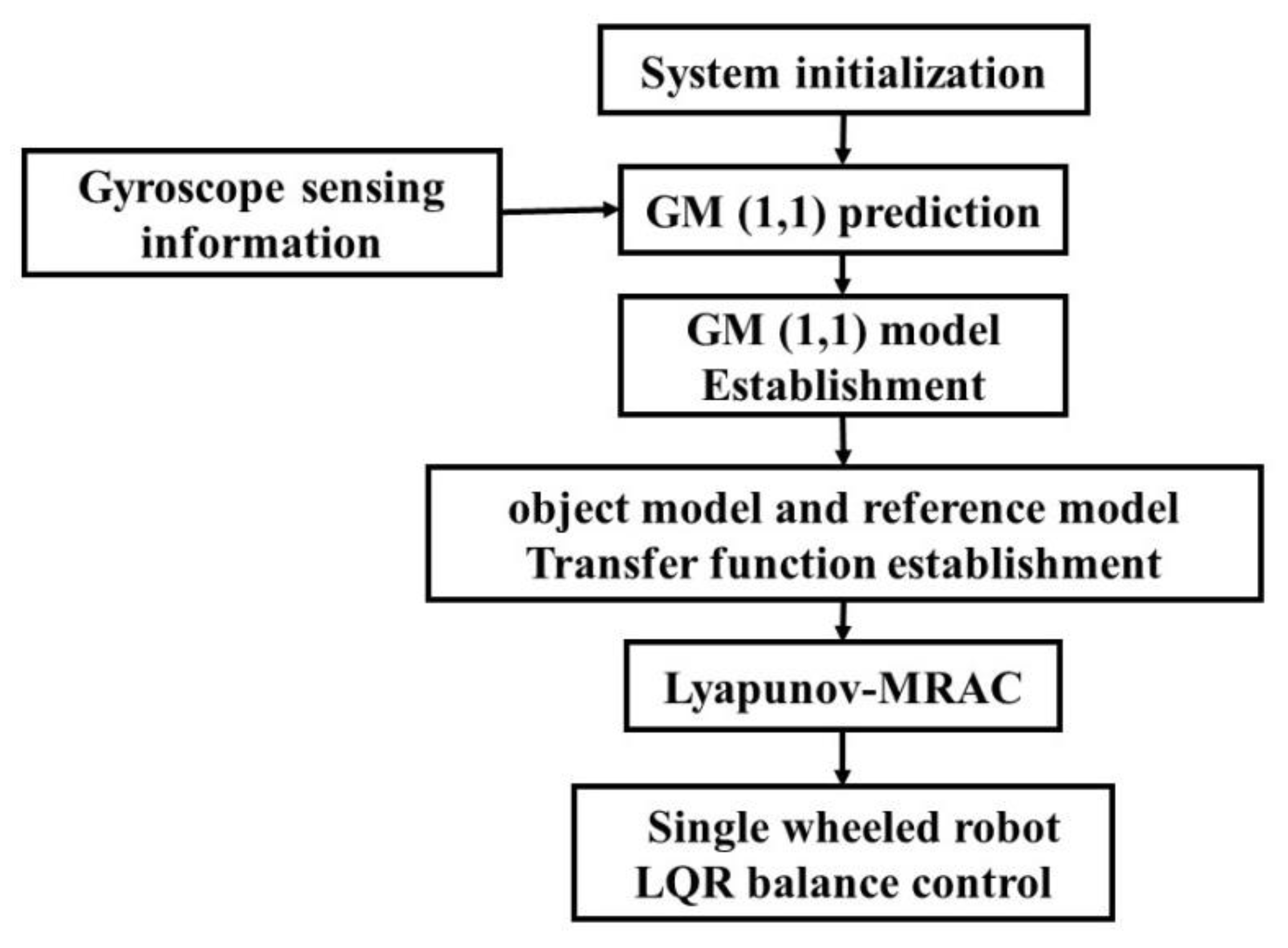
A gyroscope for measurement feedback is used to measure the change in the angle over time. Applying grey GM (1,1) for the signal prediction can serve as a reference model. A one-wheeled robot, which is a complex and unstable mechanism, can cause control difficulty. The system driver of the one-wheeled robot directly controls the robot body pendulum. The system calculates the robot’s dynamic mathematic model. GM (1,1) is employed to predict model estimation of the gyro signals. The design of the linear quadratic regulator of the robot at the stable point is conducted to verify GM (1,1) model prediction. This conforms to the control feasibility of the actual dynamic mathematic model.
GM (1,1) is applied to predict model control. It can be applied to make up for significant model deviation of the complex structure at a stable state. It serves as an adaptability application when system loading varies. For system simulation, MATLAB R2020b, a platform instrument, is utilized. Figure 4 shows the entire system structure.
Simulation shows that GM (1,1) predicts the Z-domain model equation of the gyro signal as Equation (30).
0.1103 0.2141 z 1 + 0.1038 z 2 0.1203 0.2335 z 1 + 0.1132 z 2 + 9.094 × 10 3 z 3 + 0.0003858 z 4 0.0004419 z 5
where the control parameter of a linear quadratic regulator is K = [ 83 . 97229 ,   41 . 7688 ,   26 . 3051 ,   0 . 0000 ] .
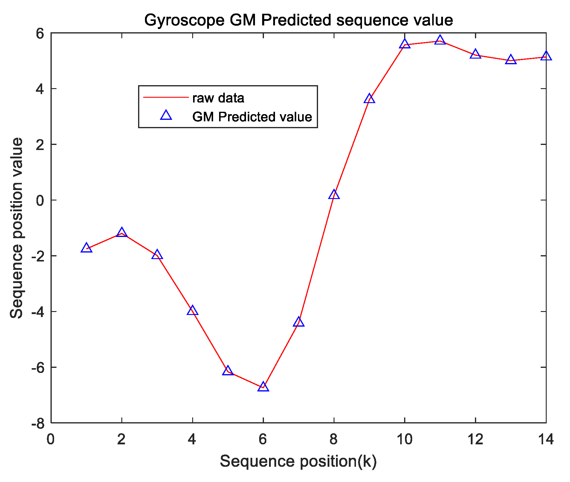
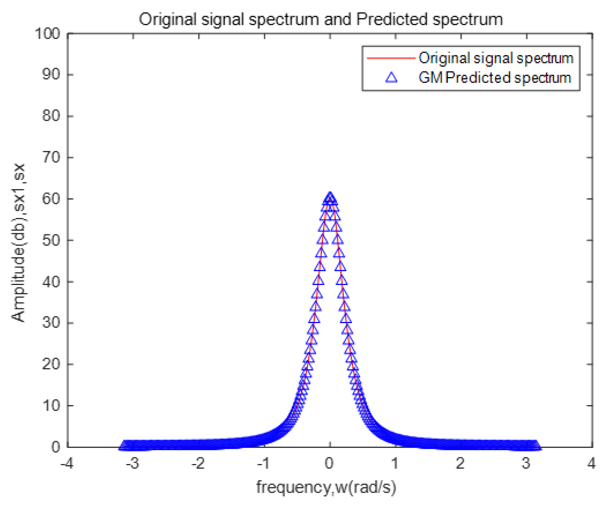
The signal measured by the gyroscope during robot movement is fitted by the gray GM (1,1) prediction numerical graph, as shown in Figure 5. This result demonstrates that the GM (1,1) can estimate state-space representation when the robot becomes balanced without any extended force or disturbance. The estimated behavior of the next moment is carried out from the present moment so that the robot can carry out robust balance control at the next moment when it is disturbed.
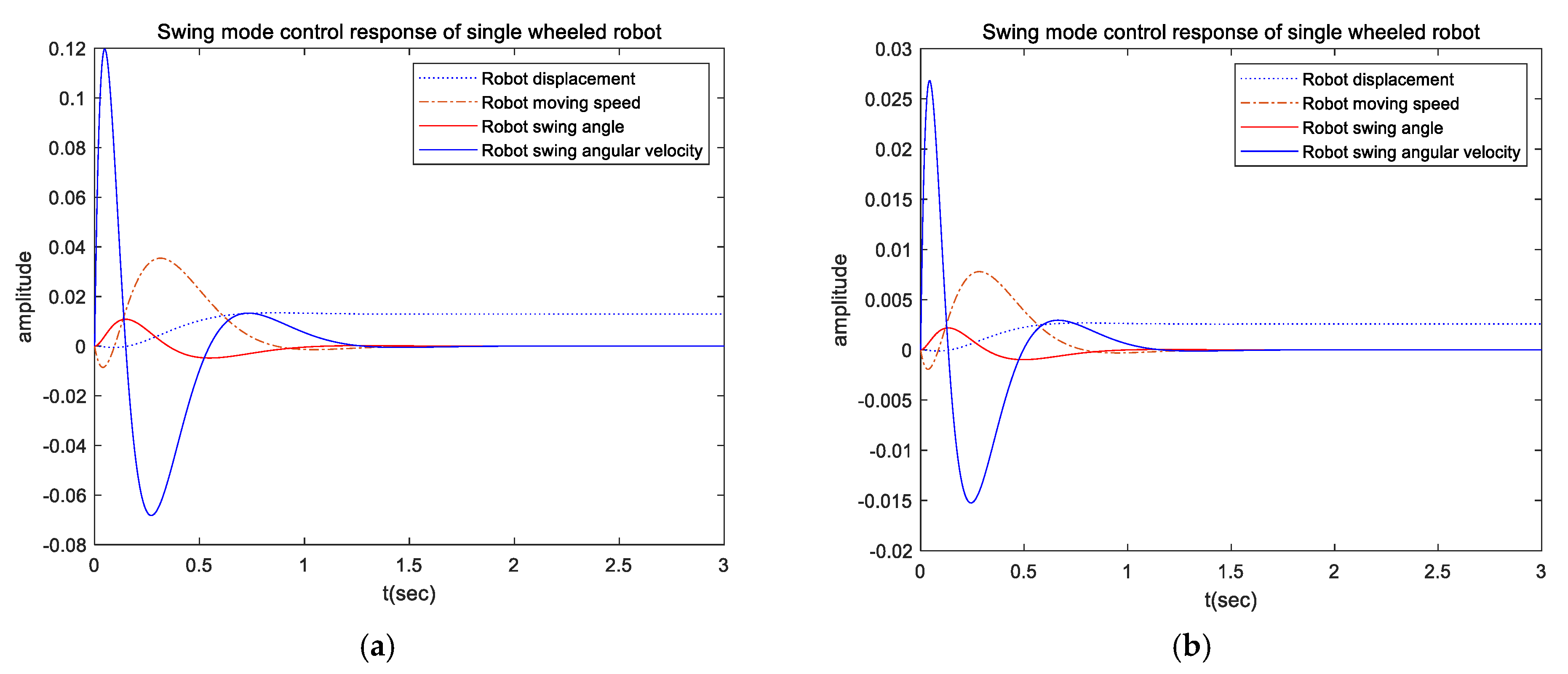
Figure 6 shows the balance’s performance by using the PID control method combined with GM (1,1) under self-swing balance and external disturbance. The results demonstrate that the overshoot of the robot’s swing angular velocity and the wheel’s velocity increase immediately under the disturbance of external force, but the performance of the dynamic balance is not affected by increasing momentum. In addition, these results verify that the control method designed in this study has excellent robustness, which can maintain the robot stability.
After the feasibility analysis, this study also simulated and verified the mathematical modeling of the robot system and the gray GM (1,1) prediction model for tracking fitting. The comparison results demonstrate that the gyroscope signal estimation of the verification system by GM (1,1) is consistent with the mathematical modeling of the robot, as shown in Figure 7. The difference between the original and predicted signals is around 0.01%, and the root-mean-square error is 1.3. Thus, the GM (1,1) can estimate the state space of the robot movement.
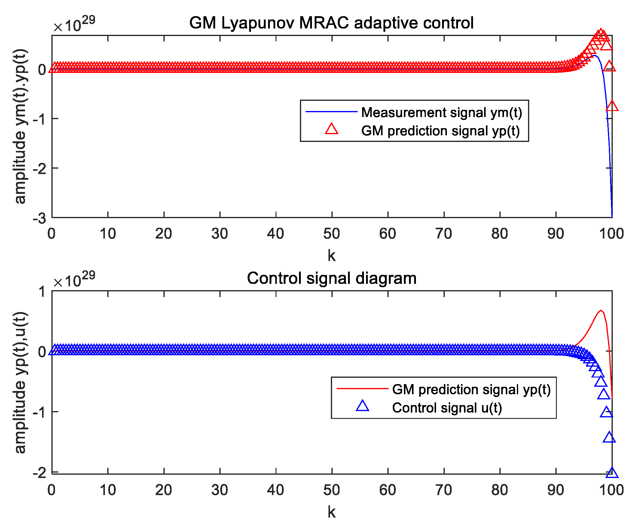
According to GM (1,1) modeling training results, the system applied GM (1,1) to the gyroscope measurement signal tracking design of Lyapunov MRAC adaptive control. It was found that the control effect of ym(t) output from the current reference model and yp(t) signal output from the existing system could be sampled by GM (1,1) estimation, and the tracking effect proved to be good. The gyroscope gray GM-Lyapunov MRAC self-tuning control and gyroscope GM (1,1) prediction equation tracking response diagrams are shown in Figure 8.
The transient response diagram of the system for GM (1,1) to achieve the balance estimation of the robot is shown in Figure 9. The results demonstrate that the system combined with GM (1,1) can estimate the state of transient response and achieve stability quickly.
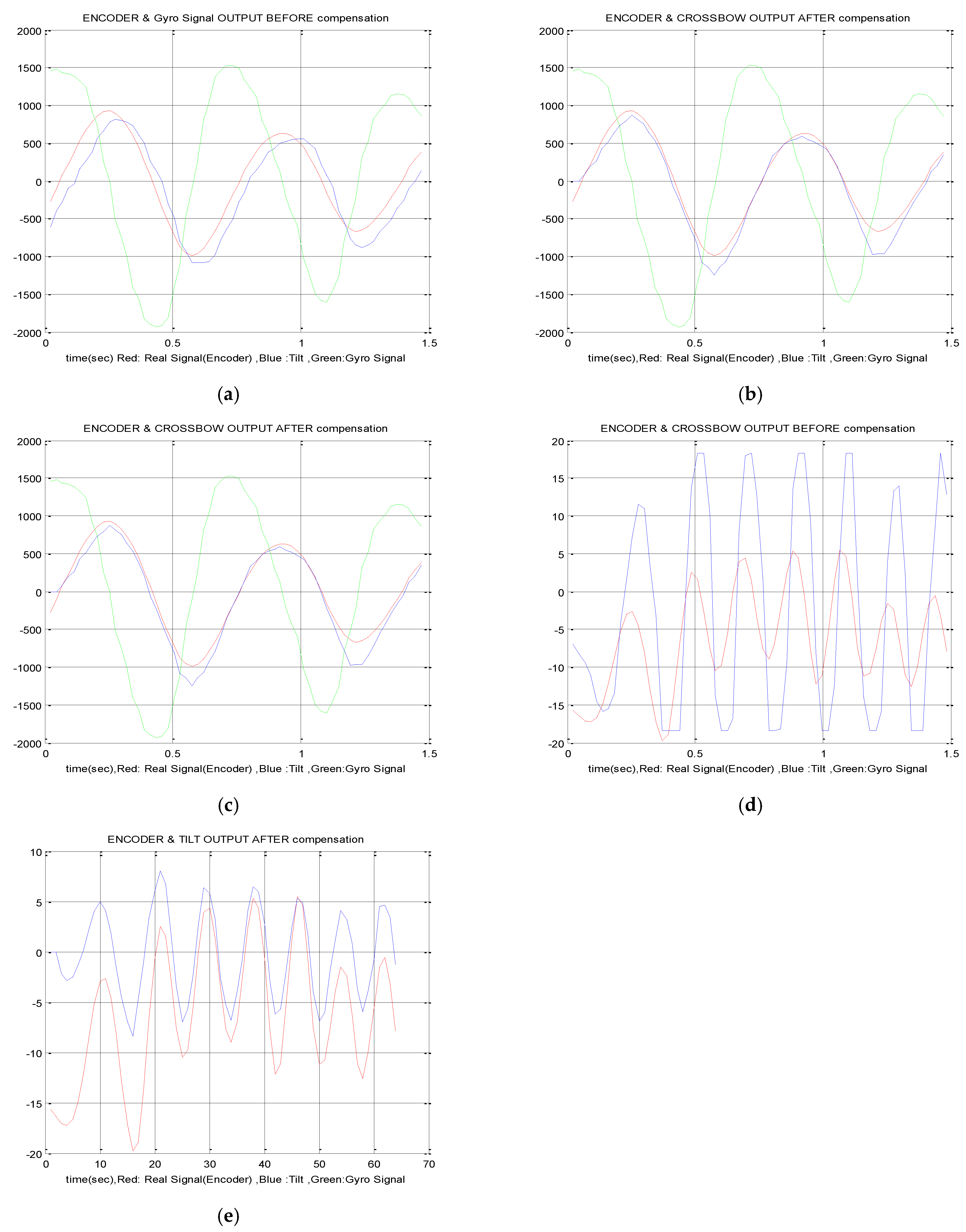
The compassion results (in Figure 10) demonstrate that PID control still has superior robustness under external disturbance. The current tiltmeter has the characteristic of time delay. The tiltmeter is designed to measure the acceleration sensor, so the accuracy of measurement will also be affected if the phenomenon of acceleration occurs on the lateral side. The response time of the tormenter is fast, but it is susceptible to noise, so it is necessary to reduce the noise interference rate of the tormenter. Therefore, this paper proposes that GM (1,1) is used to estimate the measured signals of tilting meter and tormenter to compensate for the excellent compensation effect, so the PID control algorithm can lead the single-wheel robot to achieve effective balance control quickly.

5. Conclusions

A one-wheeled robot self-balancing cart is nonlinear and lacks drive. It is a higher-order system. Based on local linearization, the paper applies all-state feedback to complete indirect control of non-driver state variables. The paper also designs an algorithm of stability control. According to simulation, the linear-quadratic regulator-based optimal control enables the self-balancing system of the one-wheeled robot to attain stability. The simulation result indicates that applying GM (1,1) can predict the gyro signal model and assess and control the feasibility of response application in the system. Using simulation to verify system control is easy and provides a quick response. Indeed, such a method is efficient.
This study mainly investigates the balance control of the single-wheeled robot. The primary control system aims to linearize the dynamic motion system by using a PID control system under an unbalanced load and then controlling the rotated velocity to adjust the inclination angle until its balance. The GM (1,1) estimated the gyroscope signal to evaluate the inclination angle of the single-wheel robot, and it also can compensate for the time delay effect rapidly from PID control. The simulation results and actual experimental results show that the application of GM (1,1) estimation is feasible; the future development direction is to reduce positioning overshoot, dynamic load change control, and load weight change control.
According to the GM (1,1) prediction, the design can optimize the one-wheeled robot motion model. However, the design does not take into concern the optimization of control rule and parameter adjustment. It fails to shorten the time for the robot to attain stability. System research is concerned with the training model of a single model. It collects only a small amount of data, thus resulting in a larger pendulum estimation error. The GM (1,1) prediction model is consequently less stable. Singularity is likely to arise and therefore affects prediction results. However, without considering the time the robot needs to attain stability, the research method still possesses better stability control ability.
To sum up, the design can be integrated with the intelligence vehicle industry. The integration can boost the unmanned control effect. Personalizing car design can indeed satisfy human needs. One-wheeled robots will be an economical and practical means of transportation. They are free from geographical constraints. Being highly mobile, they can be applied to transportation, rescue, and mineral surveys. They can generate tremendous economic benefits.

Author Contributions

Conceptualization, M.-L.C. and K.-J.C.; methodology, M.-L.C. and K.-J.C.; software, P.-H.L., M.-L.C. and K.-J.C.; validation, C.-Y.C., C.-H.W. and K.-J.C.; formal analysis, M.-L.C.; resources, C.-Y.C. and C.-H.W.; data curation, P.-H.L.; writing—original draft preparation, M.-L.C. and P.-H.L.; writing—review and editing, K.-J.C.; visualization, Pin-Hao Liao; supervision, M.-L.C. and K.-J.C.; project administration, M.-L.C. and K.-J.C. All authors have read and agreed to the published version of the manuscript.

Funding

This research received no external funding.

Acknowledgments

This research was supported by the Ningde Normal University (2018y21) high-level talent training program.

Conflicts of Interest

The authors declare no conflict of interest.

References

  1. Brown, H.B.; Xu, Y. A single-wheel, gyroscopically stabilized robot. In Proceedings of the IEEE International Conference on Robotics and Automation, Minneapolis, MN, USA, 22–28 April 1996; pp. 3658–3663. [Google Scholar]
  2. Nakajima, R.; Tsubouchi, T.; Yuta, S.; Koyanagi, E. A development of a new mechanism of an autonomous unicycle. In Proceedings of the the 1997 IEEE/RSJ International Conference on Intelligent Robot and Systems, Innovative Robotics for Real-World Applications, IROS’97, Grenoble, France, 11 September 1997; pp. 906–912. [Google Scholar]
  3. Okumura, J.; Takei, T.; Tsubouchi, T. Path tracking of an unicycle robot with a wide-type wheel aimed for navigation. In Proceedings of the 2010 11th IEEE International Workshop on Advanced Motion Control (AMC), Nagaoka, Japan, 21March 2010; pp. 268–272. [Google Scholar]
  4. Wu, C.-W.; Hwang, C.-K. A novel spherical wheel driven by Omni wheels. In Proceedings of the 2008 International Conference on Machine Learning and Cybernetics, Kunming, China, 12–15 July 2008; pp. 3800–3803. [Google Scholar]
  5. Wu, C.-W.; Huang, K.-S.; Hwang, C.-K. A novel spherical wheel driven by chains with guiding wheels. In Proceedings of the 2009 International Conference on Machine Learning and Cybernetics, Baoding, China, 12–15 July 2009; pp. 3242–3245. [Google Scholar]
  6. Patel, N.P.; Parikh, D.R.; Patel, D.A.; Patel, R.R. AI and web-based human-like interactive university chatbot (UNIBOT). In Proceedings of the 2019 3rd International conference on Electronics, Communication and Aerospace Technology (ICECA), Coimbatore, India, 12–14 June 2019; pp. 148–150. [Google Scholar]
  7. Ram, R.; Pathak, P.; Junco, S. Inverse kinematics of mobile manipulator using bidirectional particle swarm optimization by manipulator decoupling. Mech. Mach. Theory 2019, 131, 385–405. [Google Scholar] [CrossRef]
  8. Wang, L.; Pei, W.; Li, X.; Zhou, J. Research on Distributed Integrated Control Method for Wheeled Mobile Robot with Skid Steering. In Proceedings of the ISCSIC 2020: 2020 4th International Symposium on Computer Science and Intelligent Control, Newcastle upon Tyne, UK, 17–19 November 2020. [Google Scholar]
  9. Xu, Y.; Ou, Y. Control of Single Wheel Robots; Springer: Berlin/Heidelberg, Germany, 2006. [Google Scholar]
  10. Wheeler, N.J.; Jones, K.S. Kinematics affect people’s judgments of a wheeled robot’s ability to climb a stair. Int. J. Soc. Robot. 2021, 13, 117–128. [Google Scholar] [CrossRef]
  11. Bayar, G.; Ozturk, S. Investigation of The Effects of Contact Forces Acting on Rollers Of a Mecanum Wheeled Robot. Mechatronics 2020, 72, 102467. [Google Scholar] [CrossRef]
  12. Zhou, S.; Zhang, W.; Zou, Y.; Ou, B.; Xun, Z. Piezoelectric-driven miniature wheeled robot based on flexible transmission mechanisms. Microsyst. Technol. 2018, 24, 943–950. [Google Scholar] [CrossRef]
  13. Li, Z.; Deng, J.; Lu, R.; Xu, Y.; Bai, J.; Su, C.-Y. Trajectory-tracking control of mobile robot systems incorporating neural-dynamic optimized model predictive approach. IEEE Trans. Syst. Man Cybern. Syst. 2015, 46, 740–749. [Google Scholar] [CrossRef]
  14. Mathew, N.J.; Rao, K.K.; Sivakumaran, N. Swing Up and Stabilization Control of a Rotary Inverted Pendulum. IFAC Proc. Vol. 2013, 46, 654–659. [Google Scholar] [CrossRef] [Green Version]
  15. Kim, S.; Kwon, S. Dynamic modeling of a two-wheeled inverted pendulum balancing mobile robot. Int. J. Control. Autom. Syst. 2015, 13, 926–933. [Google Scholar] [CrossRef]
  16. Anoohya, B.B.; Padhi, R. Trajectory Tracking of Autonomous Mobile Robots Using Nonlinear Dynamic Inversion. IFAC-PapersOnLine 2018, 51, 202–207. [Google Scholar] [CrossRef]
  17. Zhang, X.; Ruan, X.; Xiao, Y.; Huang, J. Sensorimotor self-learning model based on operant conditioning for two-wheeled robot. J. Shanghai Jiaotong Univ. (Sci.) 2017, 22, 148–155. [Google Scholar] [CrossRef]
  18. Ruan, X.; Chen, J.; Dai, L. Motor Learning Based on the Cooperation of Cerebellum and Basal Ganglia for a Self-Balancing Two-Wheeled Robot. Intell. Control. Autom. 2011, 2, 12. [Google Scholar] [CrossRef] [Green Version]
  19. El-Bardini, M.; El-Nagar, A.M. Interval type-2 fuzzy PID controller for uncertain nonlinear inverted pendulum system. ISA Trans. 2014, 53, 732–743. [Google Scholar] [CrossRef]
  20. Liu, X.; Peng, H.; Bai, Y.; Zhu, Y.; Liao, L. Tourism Flows Prediction based on an Improved Grey GM(1,1) Model. Procedia-Soc. Behav. Sci. 2014, 138, 767–775. [Google Scholar] [CrossRef] [Green Version]
  21. Yang, S.; Luo, W.; Wang, Z.; Meng, H. Research on Highway Tunnel Ventilation Control Based on Internet of Things and Grey Prediction Algorithm. In Proceedings of the 2020 International Conference on Computer Network, Electronic and Automation (ICCNEA), Xi’an, China, 25–27 September 2020. [Google Scholar]
  22. Wardana, A.A.; Takaki, T.; Jiang, M.; Ishii, I. Development of a single-wheeled inverted pendulum robot capable of climbing stairs. Adv. Robot. 2020, 34, 674–688. [Google Scholar] [CrossRef]
  23. Jin, H.; Wang, T.; Yu, F.; Zhu, Y.; Zhao, J.; Lee, J. Unicycle Robot Stabilized by the Effect of Gyroscopic Precession and Its Control Realization Based on Centrifugal Force Compensation. IEEE/ASME Trans. Mechatron. 2016, 21, 2737–2745. [Google Scholar] [CrossRef]
  24. Forouhar, M.; Abedin-Nasab, M.H.; Liu, G. Introducing GyroSym: A single-wheel robot. Int. J. Dyn. Control 2020, 8, 404–417. [Google Scholar] [CrossRef]
  25. Lee, S.; Jung, S. Detection and control of a gyroscopically induced vibration to improve the balance of a single-wheel robot. J. Low Freq. Noise Vib. Act. Control 2017, 37, 443–455. [Google Scholar] [CrossRef]
  26. Nguyen, P.L.; Nguyen, T.P.; Ngo, T.M. Balancing control for single-wheel unicycle Robot using the Sliding mode controller. IOP Conf. Ser. Mater. Sci. Eng. 2021, 1109, 012020. [Google Scholar] [CrossRef]
  27. Zarei, F.; Moosavian, S.A.A.; Najafi, A. Force Analysis of a Spherical Single-wheeled Robot. In Proceedings of the 2018 6th RSI International Conference on Robotics and Mechatronics (IcRoM), Tehran, Iran, 23–25 October 2018; pp. 542–547. [Google Scholar]
  28. Ashwani, K.; Piyush, D.; Priyanka, S. Anti-Swing and Position Control of Single Wheeled Inverted Pendulum Robot (SWIPR). Int. J. Appl. Evol. Comput. (IJAEC) 2018, 9, 37–47. [Google Scholar] [CrossRef]
  29. Zad, H.S.; Ulasyar, A. Adaptive control of self-balancing two-wheeled robot system based on online model estimation. In Proceedings of the 2017 10th International Conference on Electrical and Electronics Engineering (ELECO), Bursa, Turkey, 30 November–2 December 2017; pp. 876–880. [Google Scholar]
  30. George, T.; Ganesan, V. Optimal tuning of PID controller in time delay system: A review on various optimization techniques. J.Chem. Prod. Process. Model. 2020, 20202001. [Google Scholar] [CrossRef]
  31. Venugopal, K.R.; Srinivasa, K.G.; Patnaik, L.M. Soft Computing for Data Mining Applications; Springer Publishing Company, Incorporated: Berlin/Heidelberg, Germany, 2009. [Google Scholar]
  32. Qian, Q.; Wu, J.; Wang, Z. Dynamic balance control of two-wheeled self-balancing pendulum robot based on adaptive machine learning. Int. J. Wavelets Multiresolut. Inf. Process. 2020, 18, 1941002. [Google Scholar] [CrossRef]
  33. Wang, Z.-X.; Li, D.-D.; Zheng, H.-H. Model comparison of GM(1,1) and DGM(1,1) based on Monte-Carlo simulation. Phys. A Stat. Mech. Appl. 2020, 542, 123341. [Google Scholar] [CrossRef]
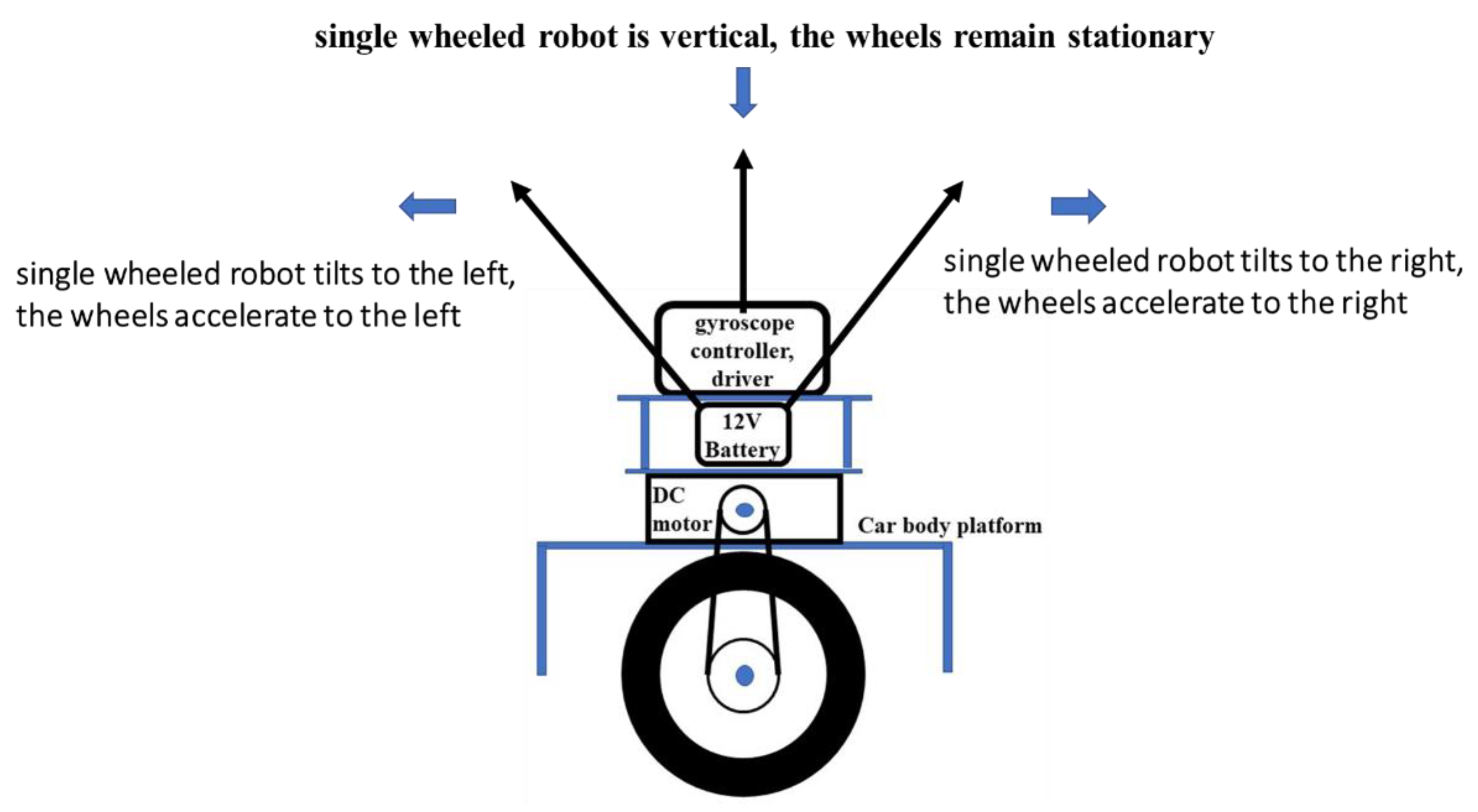
Figure 1. Single-wheeled robot motion system diagram.
Axioms 10 00326 g001
Figure 2. Force analysis of robot system.
Axioms 10 00326 g002
Figure 3. A single-wheeled robot system architecture diagram.
Axioms 10 00326 g003
Figure 4. Flowchart of GM (1,1) model in the single-wheeled robot system.
Axioms 10 00326 g004
Figure 5. Gyroscope grey GM (1,1) prediction value diagram.
Axioms 10 00326 g005
Figure 6. Swing mode control response with (a) external disturbance and (b) self-swing balance control response.
Axioms 10 00326 g006
Figure 7. Robot system mathematical modeling and grey GM (1,1) prediction mode.
Axioms 10 00326 g007
Figure 8. Gyro grey GM Lyapunov MRAC adaptive control diagram.
Axioms 10 00326 g008
Figure 9. Gyroscope GM (1,1) prediction equation transient response diagram.
Axioms 10 00326 g009
Figure 10. Control signal measurement response diagram generated under different conditions. When (a) before the tilt meter signal is compensated and (b) after the tilt meter signal is compensated, the measured signal diagram at self-equilibrium; when (c) before the tilt meter signal is compensated and (d) after the tilt meter signal is compensated, the measured signal diagram of external force interference during the balance; (e) interference signal diagram generated by external force (high frequency signal) applied to the compensated signal tilt meter.
Axioms 10 00326 g010
Table 1. All parameter symbols’ meanings.
Name of ParametersUnit
Robot body Weight (m)Kg
Robot lower body weight (M)Kg
Operating friction coefficient (b)N/(m/s)
Vehicle body to center Swing length (h)M
Body swing inertia (I)Kg
Vehicle body External force pushed (F)N
Robot position (x)kg
Robot body Swing angle (θ)rad
Gravitational acceleration (g)m/s2
Table 2. Comparison of prediction accuracy grades.
Prediction Accuracy LevelProbeC
good>0.95<0.35
qualified>0.80<0.45
reluctantly>0.70<0.50
unqualified≤0.70≥0.65
Publisher’s Note: MDPI stays neutral with regard to jurisdictional claims in published maps and institutional affiliations.