1. Introduction
Currently, two different models of power supply are available in the market, including linear power supply and switching power supply. Despite its simple circuit structure, high stability, small ripple, fast transient response, low electromagnetic interference and high reliability, linear power supply is associated with low efficiency and large size. A switching power supply is designed to compensate for the shortcomings of the linear power supply. Therefore, with technological advancements, the linear power supply has been gradually replaced by the switching power supply, which is widely used in 3C products. Despite switching power supply being credited with high conversion efficiency, light weight and a wide-range DC input, its circuit structure features a complex circuit and large electromagnetic interference. This study focuses on this phenomenon [
1,
2].
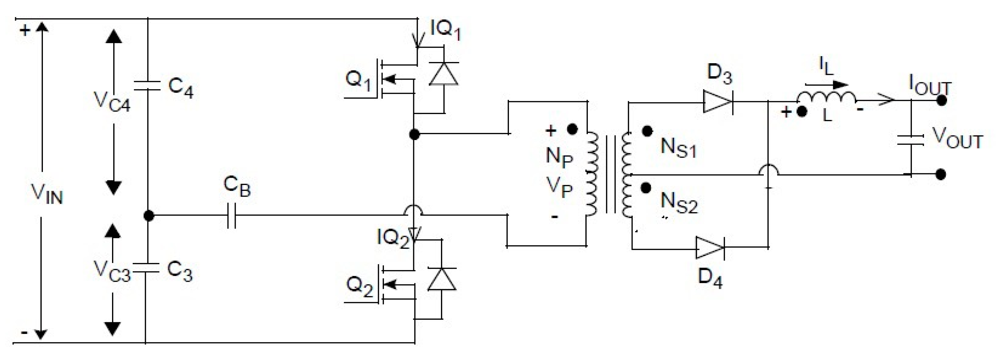
In this study, the symmetrical half-bridge power converter serves as a switching power supply. The symmetrical half-bridge power converter is different from push-pull single-ended driving or interleaved driving, which requires a double input voltage. It is widely used in converters whose power supply voltage is higher than the safety standard voltage value of the transistor.
Research on power converters has focused mainly on circuit design and practical development, including high-power two-way bridge power supplies [
3]. A high-voltage switching resonant converter has been used to reduce switching loss in the system [
4,
5,
6]. High-efficiency converters [
7,
8,
9,
10,
11] and a reluctance motor drive system for the two-way voltage double front-end converter have been developed [
12]. In battery charging applications [
13,
14,
15,
16], topology and design optimization were achieved in an optimized multiport DC/DC converter for transportation [
17,
18,
19] and a PWM in a DC/DC converter [
20,
21]. Existing studies in the literature also include a passive RF-DC converter for energy harvesting at ultra-low input power at 868 MHz [
22]; using extended Kalman filter observer technology to solve the fault problem in a DC/DC converter [
23], as well as using a DC/DC converter for e-mobility charging [
24]. Related to this study, the symmetrical half-bridge is related to high-power half-bridge converters [
25,
26,
27]. However, little research deals with the integration of the three methods. This study, therefore, can be regarded as a pioneering study of converters [
28].
The second section introduces the mathematics model employed, which includes regression analysis, the rough set method and the GM(1,N) model of grey system theory.
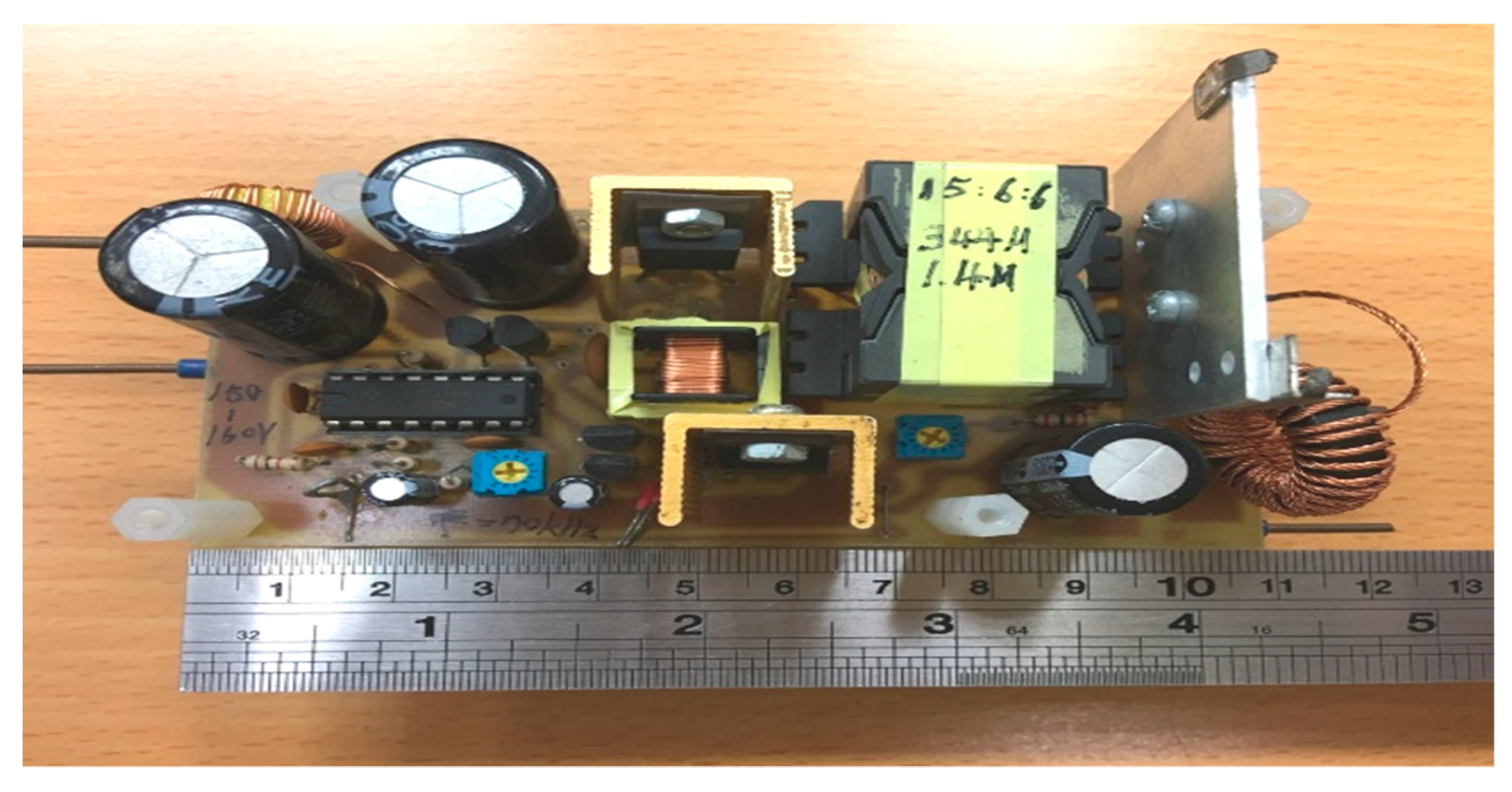
Section 3 provides a field example of a symmetrical half-bridge power converter.
Section 4 describes the complete calculation steps for the symmetrical half-bridge power converter. The final section draws conclusions from the results and puts forward suggestions for future research.
2. The Mathematical Model of Soft Computing
This section mainly describes the computing processes of regression analysis, rough set and grey GM(1,N) model. The procedure is described below.
2.1. Regression Analysis
Regression analysis is a method of statistically analyzing data. Its main purpose is to understand the relations between two or more variables and the direction and intensity of the correlation. It aims to establish a mathematical model to observe specific variables and predict the variables of interest. There are four steps in the calculation process [
29,
30].
1. List the equation
2. Expand Equation (1) to obtain
3. Transfer Equation (2) into matrix form
4. Use
to find the value of
, where
The value of is the weighting of .
2.2. Rough Set Method
Rough set is used for classification. For the affecting factors in the system, the weighting of each affecting factor to the output of the system can be obtained.
The analysis steps of rough set are as follows [
31]:
1. Information system (IS)
- i.
is called the universal set;
- ii.
is called the attribute set.
2. Information function
- i.
is called the domain of universal set;
- ii.
is called the range.
3. Discrete: based on Equation (6).
- i.
is the maximum value of the continuous attribute;
- ii.
is the minimum value of the continuous attribute.
Through the discretization, one can obtain the attribute value
where
is the representative value of discrete normalization, and
k is called the grade of discreteness.
4. Lower approximation and upper approximation
The lower approximation means that the attribute factor is completely determined to belong to U (intersection), while the upper approximation means that the attribute factor may belong to U (union).
5. Indiscernibility: For any and , they are in the same category.
6. Positive, negative and boundary
7. Dependents: The dependence of decision attribute D on conditional attribute C is
where
is the positive value of decision attribute
D.Under the conditional attribute C, the ratio of objects that can be completely classified into the whole number of objects in the set is calculated.
8. Significant: Indicates the importance of attributes in the decision-making system.
where
represents the degree of dependence between the decision attribute
D and the condition attribute
C, and calculates the importance of attribute a by using the change in value when a is removed from
C.
2.3. GM(1,N) Model
As with rough set, the GM(1,N) model is used to find the weighting of each affecting factor to the output in the system. According to the definition of grey system theory, the grey differential equation of the model is [
32]:
where:
- i.
and are coefficients;
- ii.
is a standard sequence;
- iii.
are inspected sequences;
- iv.
.
If in the sequence , is the main behavior of the system, and are the factors that affect the main behavior, the analysis step is as follows:
1. Build up original sequence
2. Build up AGO sequence
3. Transfer Equation (13) into a difference form
where
4. Based on Equation (14), we substitute the AGO data, and we obtain
Then, transfer Equation (15) into matrix form, as shown in Equation (16)
According to the least squares method, by using , we find the values
where:.
4. Calculation and Analysis
This section mainly explains the calculation process and results of three soft computing methods.
4.1. Regression Analysis
The analysis sequences are built based on the mathematics model.
Output efficiency: = (0.922, 0.944, 0.944, 0.944, 0.940, 0.935, 0.919)
The ratio of output current to input current (Io/Ii):
= (7.523810, 7.689024, 7.695122, 7.698171, 7.665049, 7.629779, 7.501695)
The ratio of output voltage to input voltage (Vo/Vi):
= (0.122684, 0.122619, 0.122619, 0.122645, 0.122594, 0.128994, 0.129019)
The ratio of output power to input power (Po/Pi):
= (0.944138, 0.944138, 0.944138, 0.939555, 0.934579, 0.918535, 0.921659)
Substitute into Equation (3) for weighting:
Use
to find the values of
, where:
The final results are shown in
Table 3.
Regression analysis shows that the actual circuit is positively correlated, while the other two are negatively correlated.
4.2. Rough Set Method
Rough set must firstly discretize the values. Accordingly, this paper discretizes the measured values into four grades.
Table 4 shows the result.
Table 4 indicates the ratio of output current to input current as
R1, the ratio of output voltage to input voltage as
R2, the ratio of output power to input power as
R3 and efficiency as decision attribute
D. Then
, the discrete data are converted into the rough set model to calculate the significance of each attribute factor.
1. Calculate the attribute set ={{},{},{},{}}
2. Calculate the decision set ; hence, = {, and substitute into Equation (9) to obtain .
3. Analyze the conditional attributes of each factor
Hence, = {}, and substitute into Equation (9) to obtain ; then, substitute into Equation (10) to obtain . Therefore, the significance of .
Hence, = {{},{},{},{},{},{},{}}, and substitute into Equation (9) to obtain ; then, substitute into Equation (10) to obtain . Therefore, the significance of .
Hence, = {{},{},{},{},{},{},{}}, and substitute into Equation (9) to obtain , and substitute into Equation (10) to obtain ; therefore, the significance of .
The final results are shown in
Table 5.
4.3. GM(1,N) Method
1. The analysis sequences are built based on the mathematical model.
Output efficiency:
= (0.922, 0.944, 0.944, 0.944, 0.940, 0.935, 0.919)
The ratio of output current to input current (Io/Ii)
= (7.523810, 7.689024, 7.695122, 7.698171, 7.665049, 7.629779, 7.501695)
The ratio of output voltage to input voltage (Vo/Vi):
= (0.122684, 0.122619, 0.122619, 0.122645, 0.122594, 0.128994, 0.129019)
The ratio of output power to input power(Po/Pi)
= (0.944138, 0.944138, 0.944138, 0.939555, 0.934579, 0.918535, 0.921659)
2. Build up AGO sequence
= (0.922, 1.866, 2.81, 3.754, 4.694, 5.629, 6.548)
= (7.5238, 15.2128, 22.908, 30.6061, 38.2712, 45.901, 53.4026)
= (0.1227, 0.2453, 0.3679, 0.4906, 0.6132, 0.7422, 0.8712)
= (0.9441, 1.8883, 2.8324, 3.772, 4.7065, 5.6251, 6.5467)
= (1.394, 2.338, 3.282, 4.224, 5.1615, 6.0885)
3. Substitute into Equation (16) to obtain the weighting
Uses to find the values of weighting where: .
The final results are shown in
Table 6.


