Article

A Shortcut Method to Solve for a 1D Heat Conduction Model under Complicated Boundary Conditions

School of Civil Engineering, Hefei University of Technology, Hefei 230009, China
*
Author to whom correspondence should be addressed.
Axioms 2022, 11(10), 556; https://doi.org/10.3390/axioms11100556
Submission received: 1 September 2022 / Revised: 29 September 2022 / Accepted: 13 October 2022 / Published: 14 October 2022
(This article belongs to the Special Issue Computational Heat Transfer and Fluid Dynamics)

Abstract

:
The function of boundary temperature variation with time, f(t) is generally defined according to measured data. For f(t), which has a complicated expression, a corresponding one-dimensional heat conduction model was constructed under the first type of boundary conditions (Dirichlet conditions) in a semi-infinite domain. By taking advantage of the Fourier transform properties, a theoretical solution was given for the model, under the condition that f(t) does not directly participate in the transformation process. The solution consists of the product of erfc(t) and f(0) and the convolution of erfc(t) and the derivative of f(t). The piecewise linear interpolation equation of f(t), based on the measured data of temperature, was substituted into the theoretical solution, thus quickly solving the model and deriving a corresponding analytical solution. Based on the analytical solution under the linear decay function boundary condition, the inflection point method and curve fitting method for calculating the thermal diffusivity were introduced and exemplified, and the variation laws of the appearance moment of the inflection point were discussed. The obtained results show that the values of thermal diffusivity calculated by the two methods are basically consistent, and that the inflection point values rise with the increasing values of the initial temperature variation of the boundary, the decrease in boundary temperature velocity, and the distance from the boundary, respectively.

1. Introduction

Joseph Fourier studied the temperature variation of a rod with an infinite length and adiabatic surface [1]. Its initial temperature is 0 °C, and the temperature remains constant with one end heated. This forms a 1D heat conduction model under Dirichlet boundary conditions in a semi-infinite domain, which has become one of the most classical heat conduction problems [2]. Current solving methods of heat conduction problems mainly include analytical and numerical methods. With the vigorous development of computer technology, the numerical method has now become the main calculation method in scientific research and engineering design [3,4,5,6,7], and the importance of an analytical solution is usually neglected. Actually, the analytical method is an important tool in the study of mathematical physics models, exhibiting the advantages of clear physical concepts, distinct physical meaning, and a reliable theoretical basis [8]. The analytical solution not only reveals the intrinsic mechanism and mathematical laws of heat conduction problems, but also provides an effective means to test the applicability and correctness of the numerical method, since the analytical solution can be approximated as an exact solution under specific boundary conditions [9]. In previous research, the function of boundary temperature, f(t) is often given with a relatively simple specific expression. Hence, many methods have been proposed to obtain analytical solutions to models for practical engineering problems basing on heat conduction equations, such as groundwater seepage [10,11], contaminant transport [12,13], and geothermal field research [14,15,16], especially using integral methods, as well as some new methods based on them. For example, we cite Laplace transform [17], Fourier transform [18], a new iteration method [19], an approximate analytical integral method [20], an integral-balance method [21], and a boundary integral method [22].
However, in real-world applications, the process of the variation of boundary temperature is sometimes complex, and it is difficult to provide a specific and accurate expression for its corresponding function f(t). For example, in a test involving the control of a material temperature field through the Dirichlet boundary, continuous manual intervention is required to effectively control the temperature variation of the tested material. Consequently, f(t) is a complex and random function of time. In this case, theoretical solutions of 1D heat conduction models in the semi-infinite domain can be obtained by utilizing certain specific properties of the integral transform. During the research of heat conduction problems with a linear heat source, Wu utilized the convolution and differential properties of the Laplace transform to provide the general theoretical solution of the model [16]. Nevertheless, the calculation process is complicated, and the given solution is complex in form and inconvenient to apply. Moreover, considering the complexity and variability of boundary conditions, some studies have examined the influence of boundary conditions on the solving process of the model and the handling of boundaries in specific problems [23,24]. When f(t) changes slowly, the sectional equivalence discrete method can be applied to solve the model based on the basic solution of the classical model [25]. However, this discrete method is unable to reveal the cumulative impact of changing boundary conditions within a specific period.
The aim of this paper is to propose a shortcut method to derive the analytical solution for a 1D heat conduction model in a semi-infinite space under the condition that the variation process of boundary temperature is complicated. Based on properties of the Fourier transform, the theoretical solution for the model is given, which is composed of commonly used functions with a relatively simple form. Subsequently, the piecewise linear interpolation function of f(t) established by temperature measurements is directly substituted into the theoretical solution to obtain the corresponding analytical solution. This method avoids the tedious deduction process; thus, the calculation process is relatively brief and easy to apply in practice. Additionally, the cumulative effect of boundary conditions can be reflected. This method of resolution can also be applied for research regarding porous media seepage and pollutant diffusion using similar models.
An important application of the derived analytical solution to the problem is to calculate thermal diffusivity by the measured temperature data. The thermal diffusivity of soil is a key element in the design of borehole heat exchangers in ground source heat pump systems [26], which reflects the variation rate of soil temperature with time. In recent years, the methods for gaining thermal diffusivity have often been divided into two categories: one is estimation based on in situ temperature records, such as infrared thermal imaging [27], photothermal beam deflection spectroscopy [28], and the Fourier spectroscopy method [29], and the other is prediction by building models, including infinite line source models [30] and semi-empirical models [31]. However, the thermal diffusivity obtained by the above methods is either estimated, or the solving process is complicated. Therefore, we propose a simple and relatively accurate method for solving the thermal diffusivity based on the analytical solution by combining the measured temperature data.

2. Basic Model

A thin-layer material with a heat source at one end is illustrated in Figure 1, which has the following characteristics:
(1)
The material is homogeneous, isotropic, and extends infinitely in the x-direction.
(2)
The material has a heat source set at one end, forming a Dirichlet boundary. The outer surface of both the material and its boundary are insulated surfaces.
(3)
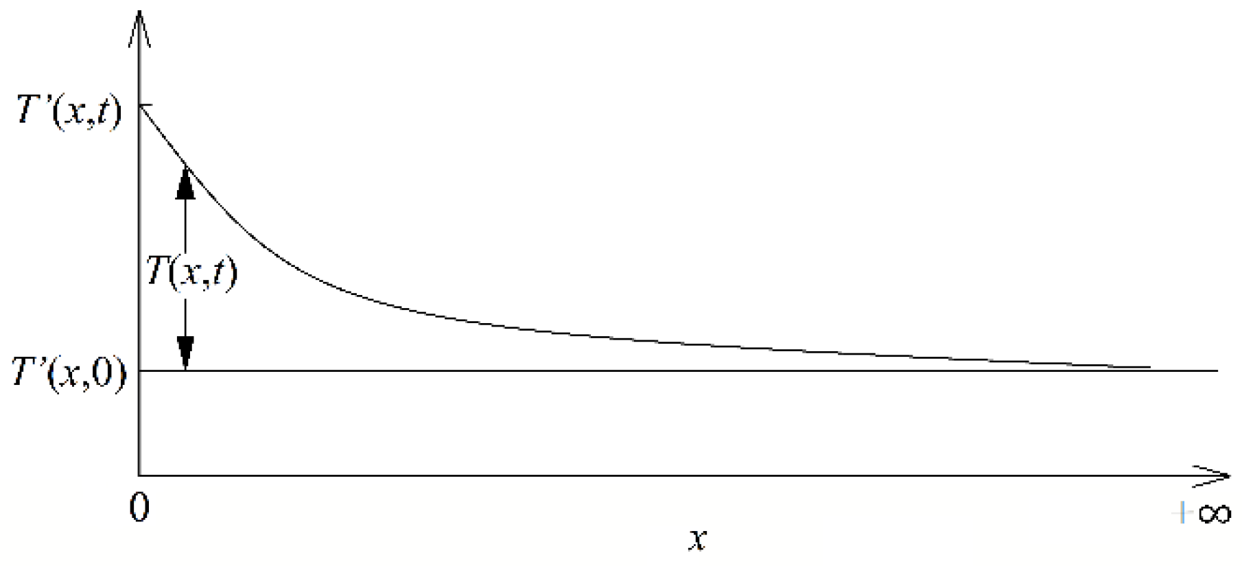
The temperature of the material at moment t from the boundary x is noted as T’(x, t), and the initial temperature of both the material and the boundary is T’(x, 0); the excess temperature at distance x from the boundary is noted as T(x,t) = T’(x,t) − T’(x,0) (as shown in Figure 2).
(4)
The excess temperature of the boundary as a function of time is denoted as f(t).
(5)
The heat transfer from the heat source to the thin-layer material is regarded as a one-dimensional process.
The heat conduction process shown above can be expressed as model (Ⅰ) as follows [2]:
T t = a 2 T x 2 0 < x < + , t > 0
T x , t t = 0 = 0 x > 0
T x , t x = 0 = f t t > 0
T x , t x = 0 t > 0
where t is the time (d), x is the distance of the calculation point from the boundary (m), T(x,t) is the excess temperature function at moment t from the boundary x (°C), f(t) is the excess temperature function of the boundary (°C), and a is the thermal diffusivity of the thin-layer material (m2/d).

3. Solutions

3.1. Theoretical Solution

According to model (Ⅰ), the variation range of x is (0, +∞); thus, the Fourier sine transform to x can be applied. Basing on the characteristics and properties of the Fourier transform, we get
F T x , t = 0 T x , t sin ω x d x = T ¯ ω , t
F T t = d T ¯ d t
F 2 T x 2 = 0 2 T x 2 sin ω x d x = ω T x = 0 ω 2 T ¯
where T ¯ is the image function for the Fourier transform on T to x, ω is the Fourier operator, and F is the Fourier transform operator.
Combining Equation (1) and the boundary condition (3), we see that
d T ¯ d t = a ω T x = 0 ω 2 T ¯ = a ω f t ω 2 T ¯
The general solution of Equation (8) is
T ¯ ω , t = exp ( ω 2 a t ) 0 t a ω f ξ · exp ( ω 2 a t ) d ξ
Considering the relationship between the inverse sine and cosine transformation and the timely exchanging integral order, T(ω,t) can be derived from Equation (9) as
T ω , t = F 1 T · ω , t = 2 π 0 exp ( ω 2 a t · 0 t a ω f ξ · exp ( ω 2 a t ) d ξ ] · sin ω x d ω = 2 π 0 t f ξ 0 ω exp ω 2 a t ξ sin ω x d ω d ξ = 2 π 0 t f ξ · { [ 1 2 a t ξ exp ω 2 a t ξ 0 + 1 2 a t ξ 0 exp ω 2 a t x cos ω x d ω } d ξ = x π 0 t f ξ t ξ 0 exp ω 2 a t ξ cos ω x d ω d ξ
where F−1 is the inverse Fourier transform operator.
The characteristic function of the Fourier transform is
0 exp a x cos θ x d x = 2 π a exp θ 2 4 a
According to Equations (10) and (11), T(x, t) can be expressed as
T x , t = x 2 π a 0 t { f ξ ( t ξ ) 3 2 · exp x 2 4 a t ξ } d ξ
Based on the definition of convolution, combined with the properties of the Fourier transform, the customary commonly used solution, expressed as a probability density function, can be obtained as
T x , t = f ξ * [ x 2 t π a t exp ( x 2 4 a t ) ] = f ξ * d d t 2 π x 2 a t + exp τ 2 d τ = f ξ * d d t erfc x 2 a t
where * is convolution operator.
From the differential property of convolution, we obtain
f t * d d t erfc x 2 a t + erfc x 2 a t | t = 0 f t = erfc x 2 a t * d f t d t + f t t = 0 · erfc x 2 a t
Because erfc x 2 a t | t = 0 =0, noting the equivalence between the third line of Equation (13) and the first term at the left side of Equation (14), Equation (14) can be written as
T x , t = f t t = 0 erfc x 2 a t + erfc x 2 a t * d f t d t
Equation (15) is the theoretical solution of the semi-infinite domain one-dimensional heat conduction model when the function of boundary condition is f(t). During the solving process, f(t) is not directly involved in the transformation, which provides a solving method for models that are difficult to solve by directly applying the Fourier transform due to the complexity of f(t).
It should be pointed out that f(t) is conducted in the form of operators during the transformation process, so f(t) should satisfy the requirements of the Fourier transform, i.e., f(t) is absolutely integrable in any time segment [32].

3.2. Analytical Solution

In order to solve the model under this condition, the continuous function of boundary condition f(t) is discretized according to the actual measurement process, without considering its specific form.
In the field of mathematics, interpolation is a method used to obtain unknown data through known discrete data in numerical analysis, and the commonly used interpolation methods are piecewise linear interpolation, Lagrange’s interpolation, Newton interpolation, and Hermite interpolation [33]. Among them, piecewise linear interpolation is the simplest interpolation method, which connects every two adjacent nodes with a straight line, so that a fold line as a piecewise linear interpolation function is formed, and the more segments that appear in a piecewise linear interpolation, the smaller the interpolation error is.
This paper adopts the piecewise linear interpolation method, which is commonly used in the engineering field to discrete f(t). This interpolation method can satisfy the computational accuracy and facilitate the solving process, and the derived solution is convenient for application. Therefore, the computational period is divided into several computational time segments. Within each time segment, f(t) is described as a linear variation function.
Initially, the temperature of the boundary is consistent with that of the material, and then the boundary temperature suddenly changes by ΔT0, followed by a change in a certain law. Assuming that ΔT0 is formed instantaneously and its duration is negligible, namely f(0) = ΔT0, the interpolation on f(t) can be conducted by regarding ΔT0 as the reference point, as illustrated in Figure 3, and the temperature variation in the i-th time segment (between time points ti-1 and ti), fi(t), can be expressed as
f i t = f i 1 + f i f i 1 t i t i 1 t t i 1
where fi is the boundary temperature at the end of the i-th time segment (or at the time point ti) and ti−1 < t < ti, I ϵ N*.
Thus, f(t) can be written as
f t = Δ T 0 + i = 1 n β i t t i 1 · H t t i 1
where βi = (fi − fi−1)/(ti − ti−1), tti−1, I ϵ N*, and H(tti−1) is the Heaviside function, when t < ti−1, H(t − ti−1) = 0, when tti-1, H(t − ti−1) = 1.
Substituting Equation (17) into Equation (15) leads to
T x , t = f t t = 0 erfc x 2 a t + erfc x 2 a t * i = 1 n β i · H t t i 1
Considering f(0) = ΔT0 and that the property of H(tti−1) when tti−1, gives
T x , t = Δ T 0 erfc x 2 a t + i = 1 n β i t i 1 t erfc x 2 a ζ d ζ
Equation (19) is the analytical solution to this sort of problem.

3.3. Specific Analytical Solutions under Particular Conditions

3.3.1. f(t) = ΔT0

This boundary condition means that the corresponding temperature of the boundary instantaneously changed by ΔT0, followed by maintaining stability, i.e., I = 0. Therefore, the second item at the right end of Equation (19) is pointless, and Equation (19) converts to the solution of the classical model for this sort of problem.

3.3.2. ΔT0 ≠ 0 ∩ i = 1

At this point, ti−1 = 0, t1 > 0 and Equation (17) becomes
f t = Δ T 0 + β t t 1
where tt1.
This condition means that the boundary temperature f(t) changes instantaneously by ΔT0 and remains constant until t1, followed linear variation at a rate of β (β > 0 means the temperature rises, and β < 0 means the temperature falls). Then, T(x,t) can be written as
T x , t = Δ T 0 erfc x 2 a t + β t 1 t erfc x 2 a ζ d ζ
The phenomenon that the boundary temperature rapidly changes at the beginning and then slowly recovers to the initial temperature is common in practice. For example, in a heat pipeline or an oil pipeline that needs to be heated in winter, the temperature of the pipeline and its internal fluid rises rapidly at the beginning of the heating period and then decreases as the heat supply gradually reduces until the next heating period, when the pipeline temperature reaches the design value [34].
It should be noted that when t1 = 0, which means f(t) starts to change slowly with a rate of β, following an instantaneous variation of ΔT0, i.e., f(t) = ∆T0 + βt, then T(x,t) can be expressed as
T x , t = Δ T 0 erfc x 2 a t + β 0 t erfc x 2 a ζ d ζ
The excess temperature variation rate at distance x from the boundary, φ(x,t) = ∂T(x,t)/∂t can be derived from Equation (22) as
φ x , t = Δ T 0 2 π a t 3 exp x 2 4 a t + β erfc x 2 4 a t
For the point at distance x from the boundary, the excess temperature variation rate caused by β is recorded as φβ(x,t), which can be resolved through Equation (23) under the condition that ΔT0 = 0, and the excess temperature response caused by ΔT0 is denoted as T0(x,t), which can be derived from Equation (22) under the condition that β = 0. Both φβ(x,t) and T0(x,t) contain erfc( x / 2 a t ), meaning that φβ(x,t) has a variation rule identical to that of T0(x,t), which also reflects the cumulative effect of β on T(x,t).
Particularly, when β < 0, meaning that f(t) decays slowly and linearly after an instantaneous variation of ΔT0, this type of condition is called the linear decay function boundary.

4. Methods

Based on temperature data obtained in the experiment, the analytical solution of the heat conduction model under the linear decay function boundary condition is applied to solve for the thermal diffusivity of soil by using principles of the inflection point method and the curve fitting method.

4.1. Curve Fitting Method

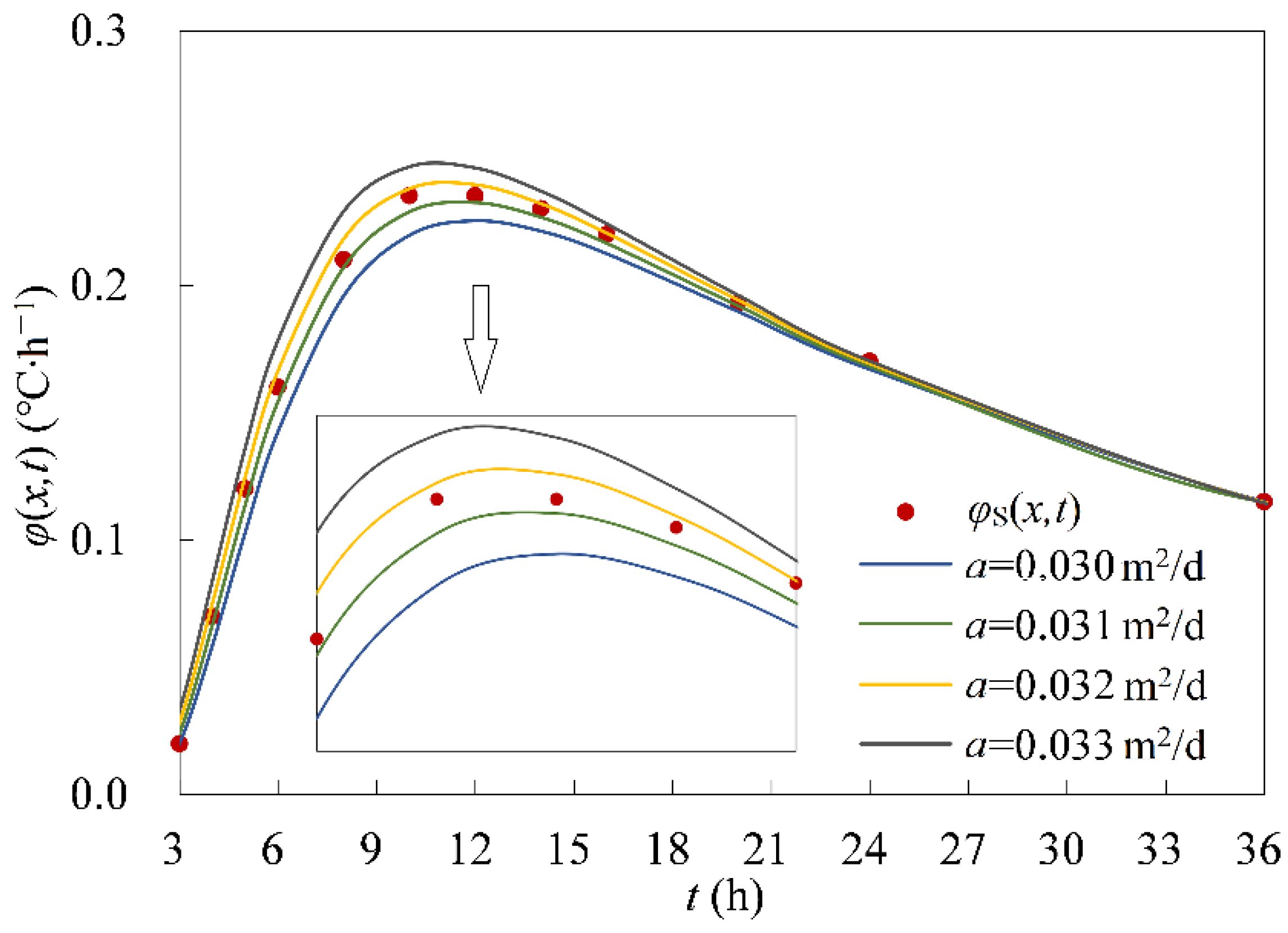
The curve fitting method is a simple and convenient method for parameter estimation, avoiding the systematic calculation errors caused by traditional parameter estimation methods, such as the traditional moment method and the maximum likelihood method; thus, it is widely used in the field of hydrogeology [35]. For a temperature measurement point at distance x from the boundary, where the value of x is fixed, φt(x,t) can be calculated for different values of a at different moments t by Equation (23), from which a family of theoretical curves corresponding to different a values, φt(x,t) − t can be drawn. Meanwhile, from the measured data at the temperature measurement point, the measured temperature variation rate curve, φm(x,t) − t can be drawn.
When the value of a in the φm(x,t) − t curve is identical to that of a curve in the φt(x,t) − t theoretical family, the two curves should have the same shape and overlap exactly. According to this principle, the value of a in the specimen can be determined by the curve-fitting process of the measured φm(x,t) − t curve and the theoretical φt(x,t) − t curve family.

4.2. Inflection Point Method

The inflection point method is a method of plotting curves according to actual measurement data and using its inflection point to graphically solve for parameters [36]; this method is widely applied in many fields, including civil engineering, chemistry, and hydrogeology.
According to Equation (23), we have
φ x , t t = 1 2 π a t 3 exp ( x 4 a t ) Δ T 0 t 3 2 + x 2 4 a t + β
It can be seen from Equation (24) that an inflection points exist on the φ(x,t) − t curve. Let us denote the time corresponding to inflection points as tg, which can be calculated by tg = 0 as
t g = Δ T 0 2 β 3 2 ( 3 2 ) 2 β / Δ T 0 x 2 a
t g = Δ T 0 2 β 3 2 + ( 3 2 ) 2 β / Δ T 0 x 2 a
When the value of x is fixed, the variation process of φ(x,t) with time can be drawn as the φ(x,t) − t curve.
It should be noted that, regardless of the positive or negative of β, under the boundary condition, which is a monotonic function with ΔT0 and β as fixed values, there cannot be two inflection points on the φ(x,t) − t curve at any point. That is, only one of the Equations (25) and (26) regarding tg is reasonable. From Equation (26), when β < 0, tg < 0, this is not consistent with the physical meaning of the problem, i.e., Equation (26) is not universal. The calculation result of Equation (25) does not produce the above contradiction, i.e., Equation (25) is universal.
According to the inflection point tg of the measured φ(x,t) − t curve, the model parameter a can be calculated from Equation (25), when combined with the measured ΔT0, β, and x in the test.

5. Results

A soil specimen (d = 3.0 m, b = 1.5 m, c = 0.3 m, as shown in Figure 1) is taken from an observation hole buried at a depth of about 20 m in a ground source heat pump project in Hefei City. A steel pipe with an outside diameter of 0.15 m is pre-set at one end as a heat source. The steel pipe and the specimen are protected by heat insulation material. Two temperature measurement fibers are set in the specimen at 0.3 m and 0.5 m from the steel pipe, respectively.
In a test lasting two days, the initial temperature of the specimen is 17.97 °C. At the initial stage of the test, hot water of 36 °C is poured into the steel pipe quickly, then the water temperature is slowly decreased at an approximately constant rate by the resistance heater. At the end of the test, the water temperature reaches 35.5 °C. Thus, ΔT0 = 18.03 °C, β = −0.25 °C/d. The results of the measured Tm(x,t) of measurement point 1 at 0.3 m from the heat source are given in Table 1.

5.1. Curve Fitting Method

The curve fitting process is illustrated in Figure 4.
As shown in Figure 4, the points on the measured curve φm(x,t) – t are approximately in the middle of the theoretical curve φt(x,t) – t, with a = 0.031 m2/d and a = 0.032 m2/d. Hence, the value of a can be determined as 0.0315 m2/d.
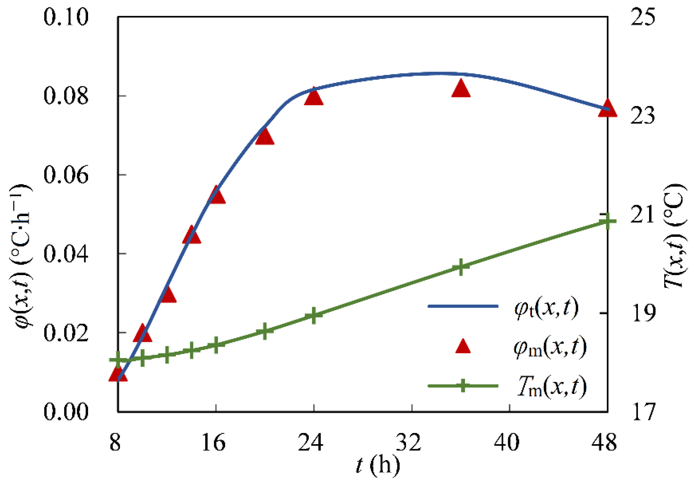
Substituting a = 0.0315 m2/d into Equation (23), the temperature variation process of measurement point 2 can be calculated. We compare the calculation results with the measured data to verify the reliability of the calculated parameter value and the rationality of the test process.
The results of the measured Tm(x,t) of measurement point 2 at 0.5 m from the heating device are given in Table 2 and Figure 5.
From Table 2 and Figure 5, it can be seen that the measured curve φm(x,t) − t and the theoretical curve φt(x,t) − t at measurement point 2 fit well, indicating that the value of a derived from the temperature data of measurement point 1 is reliable.

5.2. Inflection Point Method

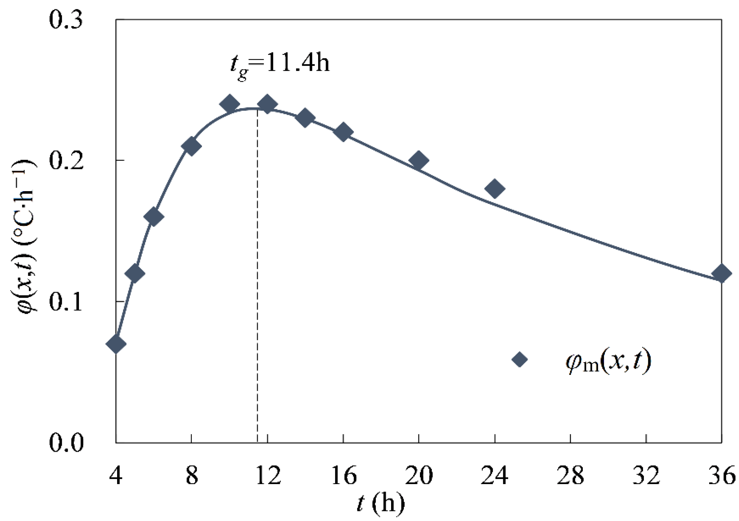
The φm(x,t) − t curve of measurement point 1 is illustrated in Figure 6.
Figure 6 shows that the inflection point of the φm(x,t) − t curve, tg appears at 11.4 h or 0.475 d. According to Equation (25), the value of a is calculated as 0.0314 m2/d.

6. Discussion

6.1. Comparison to Traditional Solving Method

When the variation process of f(t) is complicated, and its expression is outside the range of the existing Fourier transform table, or the product of the image function of f(t) and the solution of the ordinary differential equation is not within the range of the existing inverse Fourier transform table, it will be very difficult to solve the problem using the traditional Fourier transform method.
The method proposed in this paper to derive the theoretical solution using the Fourier transform property and to obtain the analytical solution by substituting the piecewise linear interpolation equation of boundary temperature into the theoretical solution can effectively solve the above problem. It should be noted that when the form of f(t) is relatively simple, such as a constant or an exponential function, the analytical solution can be obtained by substituting f(t) into the theoretical solution directly, thus quickly solving the problem.

6.2. Comparison of Thermal Diffusivity Obtained by the Two Methods

From Section 5, it can be seen that the values of a given by the curve fitting method and the inflection point method are basically consistent, and are within the range of empirical values of a in the location of the project [16].

6.3. Variation Laws of the Appearance Moment of the Inflection Point

As indicated in Equation (25), the appearance moment of the inflection point, tg, is related to the parameters of ΔT0, β, x, and a. Now set the value of a as a fixed value, i.e., 0.0314 m2/d, and the variation rules of tg with other three parameters are discussed subsequently.
The corresponding results of inflection point tg at different value of ΔT0, β, and x, calculated by Equation (25), are listed in Table 3, Table 4 and Table 5.
Table 3, Table 4 and Table 5 show that the corresponding results of tg rise with the increasing values of ∆T0, β, and x, respectively; that is, the higher the initial temperature of the heat source, the slower the temperature of the heat source decreases, and the further away from the heat source, then the later the inflection point of the temperature variation velocity curve φ(x,t) − t appears. Moreover, tg rises more significantly with the increasing value of x than that of ∆T0 and β; the detailed variation process is illustrated in Figure 7.

7. Conclusions

In this paper, we presented a new method for deriving analytical solutions for a 1D heat conduction model and its application for computing thermal diffusivity. The main findings are summarized as follows.
  • When it is difficult to give a specific and accurate expression for boundary temperature, due to its complicated variation process, the properties of the Fourier transform and the differential characteristic of the convolution integral can be fully utilized for deriving the theoretical solution to the 1D heat conduction model, without considering the detailed transformation process of f(t). In addition, the piecewise linear interpolation method is adopted to discretize the actual temperature variation process, followed by substituting the interpolation function into the theoretical solution, thus providing a shortcut method to obtain a solution composed of more commonly used functions with a relatively simple form. For the study of similar problems based on this sort of heat conduction model, this resolving method can also be referenced.
  • Based on the derived solution and the variation characteristics of the temperature variation rate φ(x,t) with time t, the curve fitting method and the inflection point method used to calculate the thermal diffusivity a are given, and the values of a calculated by the two methods are basically consistent.
  • For a certain material (i.e., a is a fixed value), the higher the initial temperature of the heat source, the slower the temperature of the heat source decreases, and the further away from the heat source, then the later the inflection point of the φ(x,t)-t curve (the curve of temperature variation velocity curve at distance x from the boundary with time t) appears.

Author Contributions

Conceptualization, T.W. and Y.T.; methodology, T.W.; validation, T.W.; formal analysis, T.W. and Y.T.; investigation, T.W.; resources, Y.T.; data curation, T.W.; writing—original draft preparation, T.W.; writing—review and editing, Y.T.; visualization, T.W.; supervision, Y.T.; project administration, H.R.; funding acquisition, F.L. All authors have read and agreed to the published version of the manuscript.

Funding

This research was funded by the Open Research Fund Program of the State Key Laboratory of Hydroscience and Engineering, Tsinghua University, grant number sklhse-2020-D-06.

Institutional Review Board Statement

Not applicable.

Informed Consent Statement

Not applicable.

Data Availability Statement

Not applicable.

Conflicts of Interest

The authors declare no conflict of interest.

Nomenclature

athermal diffusivity, m2/d
fboundary temperature, °C
FFourier transform operator
F−1inverse Fourier transform operator
ttime, d
tgthe appearance moment of inflection point, h
Ttemperature of calculation point, °C
T ¯ image function for Fourier transform
ΔT0instantaneous change of boundary temperature, °C
xdistance from the boundary of the calculation point, m
βboundary temperature variation rate, °C/d
φtemperature variation rate of the calculation point, °C/h
ωFourier operator
*convolution operator

References

  1. Fourier, J. The Analytical Theory of Heat; Peking University Press: Beijing, China, 2008; pp. 90–91. [Google Scholar]
  2. Carslaw, H.S.; Jaeger, J.C. Conduction of Heat in Solids; Oxford University Press: Oxford, UK, 1986; pp. 62–64. [Google Scholar]
  3. Asogwa, K.K.; Goud, B.S.; Shah, N.A.; Yook, S. Rheology of electromagnetohydrodynamic tangent hyperbolic nanofluid over a stretching riga surface featuring dufour effect and activation energy. Sci. Rep. 2022, 12, 14602. [Google Scholar] [CrossRef] [PubMed]
  4. Bejawada, S.G.; Jamshed, W.; Safdar, R.; Reddy, Y.D.; Alanazi, M.M.; Zahran, H.Y.; Eid, M.R. Chemical reactive and viscous dissipative flow of magneto nanofluid via natural convection by employing Galerkin finite element technique. Coatings 2022, 12, 151. [Google Scholar] [CrossRef]
  5. Goud, B.S. Thermal radiation influences on MHD stagnation point stream over a stretching sheet with slip boundary conditions. Int. J. Sci. Technol. 2020, 7, 70201. [Google Scholar] [CrossRef]
  6. Kumar, P.P.; Goud, B.S.; Malga, B.S. Finite element study of Soret number effects on MHD flow of Jeffrey fluid through a vertical permeable moving plate. Part. Differ. Equ. Appl. Math. 2020, 1, 100005. [Google Scholar] [CrossRef]
  7. Shankar Goud, B. Heat generation/absorption influence on steady stretched permeable surface on MHD flow of a micropolar fluid through a porous medium in the presence of variable suction/injection. Int. J. Thermofluids 2020, 7–8, 100044. [Google Scholar] [CrossRef]
  8. Hu, X.; Deng, S.; Wang, Y.; Chen, J.; Zhang, L.; Guo, W.; Han, Y. Study progress on analytical solution of static temperature field with artificial ground freezing. Mine Constr. Technol. 2015, 36, 1–9. [Google Scholar]
  9. Xie, H.; Zhang, C.; Jiang, Y. An analytical solution to organic contaminants diffusion through composite liners consisting of a geomembrane,a GCL and an attenuation layer considering degradation. J. Hydraul. Eng. 2014, 45, 52–60. [Google Scholar]
  10. Suk, H.J.; Chen, J.S.; Park, E.Y.; Kihm, Y.H. Practical Application of the Galerkin Finite Element Method with a Mass Conservation Scheme under Dirichlet Boundary Conditions to Solve Groundwater Problems. Sustainability 2020, 12, 5627. [Google Scholar] [CrossRef]
  11. Shah, N.A.; Rauf, A.; Vieru, D.; Sitthithakerngkiet, K.; Kumam, P. Analytical Solutions of the Diffusion–Wave Equation of Groundwater Flow with Distributed-Order of Atangana–Baleanu Fractional Derivative. Appl. Sci. 2021, 11, 4142. [Google Scholar] [CrossRef]
  12. Falta, R.W.; Wang, W.W. A semi-analytical method for simulating matrix diffusion in numerical transport models. J. Contam. Hydrol. 2017, 197, 39–49. [Google Scholar] [CrossRef] [Green Version]
  13. Zhou, Q.; Oldenburg, C.M.; Rutqvist, J. Revisiting the analytical solutions of heat transport in fractured reservoirs using a generalized multirate memory function. Water Resour. Res. 2019, 55, 1405–1428. [Google Scholar] [CrossRef]
  14. BniLam, N.; Al-Khoury, R.; Shiri, A.; Sluys, L.J. A semi-analytical model for detailed 3D heat flow in shallow geothermal systems. Int. J. Heat Mass Transf. 2018, 123, 911–927. [Google Scholar] [CrossRef]
  15. Li, Y.; Shu, L.; Xiao, R.; Tao, Y.; Niu, S.; Wang, Z. Effect of pumping-recharge well structures on heat transfer characteristics of double-well groundwater heat pump systems considering hydrothermal coupling. Energy Convers. Manag. 2021, 249, 114871. [Google Scholar] [CrossRef]
  16. Wu, D. Study on Heat Transfer Model of High Efficient Heat Exchange System in Ground Source Heat Pump. Ph.D. Dissertation, Hefei University of Technology, Hefei, China, 2019. [Google Scholar]
  17. Povstenko, Y.; Klekot, J. Fractional heat conduction with heat absorption in a sphere under Dirichlet boundary condition. Comput. Appl. Math. 2018, 37, 4475–4483. [Google Scholar] [CrossRef] [Green Version]
  18. Hua, Y.C.; Zhao, T.; Guo, Z.Y. Optimization of the one-dimensional transient heat conduction problems using extended entransy analyses. Int. J. Heat Mass Transf. 2018, 116, 166–172. [Google Scholar] [CrossRef]
  19. Huang, D.; Li, Y.; Pei, D. Identification of a time-dependent coefficient in heat conduction problem by new iteration method. Adv. Math. Phys. 2018, 2018, 4918256. [Google Scholar] [CrossRef]
  20. Kot, V.A. Integral method of boundary characteristics: The Dirichlet condition. Principles. Heat Transf. Res. 2016, 47, 1035–1055. [Google Scholar] [CrossRef]
  21. Fabre, A.; Hristov, J. On the integral-balance approach to the transient heat conduction with linearly temperature-dependent thermal diffusivity. Heat Mass Transf. 2017, 53, 177–204. [Google Scholar] [CrossRef]
  22. Kot, V.A. Integral method of boundary characteristics in solving the Stefan problem: Dirichlet condition. J. Eng. Phys. Thermophys. 2016, 89, 1289–1314. [Google Scholar] [CrossRef]
  23. Dell’Oro, F.; Goubet, O.; Mammeri, Y.; Pata, V. A semidiscrete scheme for evolution equations with memory. Discret. Contin. Dyn. Syst. 2019, 39, 5637–5658. [Google Scholar] [CrossRef] [Green Version]
  24. Gasilov, N.A.; Amrahov, S.E.; Fatullayev, A.G. On a solution of the fuzzy Dirichlet problem for the heat equation. Int. J. Therm. Sci. 2016, 103, 67–76. [Google Scholar] [CrossRef]
  25. Zhang, W.Z. Calculation of Unsteady Flow of Groundwater and Evaluation of Groundwater Resources; Science Press: Beijing, China, 1983; pp. 222–224. [Google Scholar]
  26. Shan, K.; Zhang, X.S.; Li, S.H. A method for measuring thermal properties of ground. Acta Energ. Sol. Sin. 2010, 31, 22–26. [Google Scholar]
  27. Kodikara, J.; Rajeev, P.; Rhoden, N.J. Determination of thermal diffusivity of soil using infrared thermal imaging. Can. Geotech. J. 2011, 48, 1295–1302. [Google Scholar] [CrossRef]
  28. Proskurnin, M.A.; Korte, D.; Rogova, O.B.; Volkov, D.S.; Franko, M. Photothermal Beam Deflection Spectroscopy for the Determination of Thermal Diffusivity of Soils and Soil Aggregates. Int. J. Thermophys. 2018, 39, 10765. [Google Scholar] [CrossRef]
  29. Beardsmore, G.; Egan, S.; Sandiford, M. A Fourier Spectral Method to Measure the Thermal Diffusivity of Soil. Geotech. Test. J. 2020, 43, 20180300. [Google Scholar] [CrossRef]
  30. Yoon, S.; Kim, M. Prediction of ground thermal diffusivity from thermal response tests. Energy Build. 2019, 185, 239–246. [Google Scholar] [CrossRef]
  31. Carson, J.K. A Versatile Effective Thermal Diffusivity Model for Porous Materials. Int. J. Thermophys. 2021, 42, 141. [Google Scholar] [CrossRef]
  32. Teng, Y.M. Some problems in integeral transform. Coll. Math. 2015, 31, 105–109. [Google Scholar]
  33. Zhang, Y.H.; Xi, M.C.; Chen, X.Q. Numerical Calculation Method and Algorithm; Science Press: Beijing, China, 2002; Volume 73, pp. 9–27. [Google Scholar]
  34. Li, G.; Sheng, Y.; Jin, H.; Ma, W.; Qi, J.; Wen, Z.; Zhang, B.; Mu, Y.; Bi, G. Forecasting the oil temperatures along the proposed China-Russia Crude Oil Pipeline using quasi 3-D transient heat conduction model. Cold Reg. Sci. Technol. 2010, 64, 235–242. [Google Scholar] [CrossRef]
  35. Zhou, C.; Chen, Y.; Wei, L.; Cheng, L.; Huang, Q.; Cao, X. Application of fitting-curve method to frequency analysis of POT flood series. Water Resour. Power 2011, 29, 48–50. [Google Scholar]
  36. Zeng, Q.; Mo, H.; Liu, J. Inflection point method to analyze the stability of soft soil embankment during construction. J. China Foreign Highw. 2006, 26, 21–25. [Google Scholar]
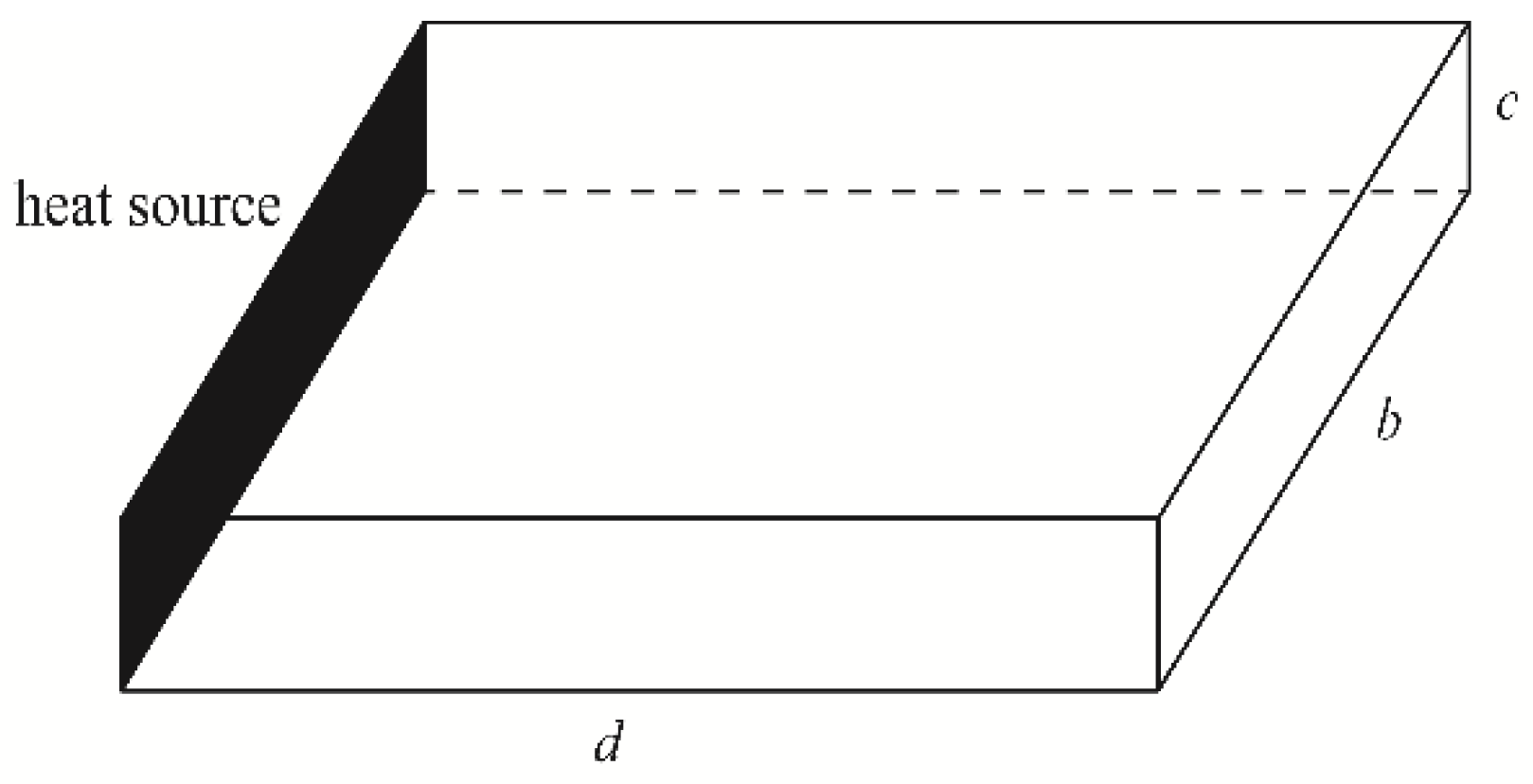
Figure 1. Sketch map of the thin-layer material.
Axioms 11 00556 g001
Figure 2. Sketch map of the variation of T(x,t).
Axioms 11 00556 g002
Figure 3. Illustration of discretization of f(t).
Axioms 11 00556 g003
Figure 4. Curve fitting method for resolving a.
Axioms 11 00556 g004
Figure 5. Comparison diagram of φm(x,t) − t and φt(x,t) − t at measurement point 2.
Axioms 11 00556 g005
Figure 6. The inflection point of the measured φm(x,t) − t curve at measurement point 1.
Axioms 11 00556 g006
Figure 7. Curves of φ(x,t) − t at different values of x.
Axioms 11 00556 g007
Table 1. Tm(x,t) and φm(x,t) of measurement point 1 (x = 0.3 m).
t (h)Tm(x,t) (°C)φm(x,t) (°C∙h−1)
3 *18.030.020
418.100.070
518.220.120
618.380.160
818.800.210
1019.270.235
1219.740.235
1420.200.230
1620.640.220
2021.410.193
2422.090.170
36 *23.470.115
* The temperature variation at measurement point 1 is not significant during the first 2 h and last 12 h of the test; thus, relative measurements are not listed.
Table 2. Tm(x,t), φm(x,t) and φt(x,t) of measurement point 2 (x = 0.5 m).
t (h)Tm(x,t) (°C)φm(x,t) (°C∙h−1)φt(x,t) (°C∙h−1)
8 *18.050.0100.008
1018.090.0200.019
1218.150.0300.032
1418.240.0450.045
1618.350.0550.056
2018.630.0700.072
2418.950.0800.082
3619.930.0820.085
4820.860.0770.077
* The temperature change at measurement point 2 is not significant during the first 7 h of the test; thus, the corresponding measurement data are not included.
Table 3. Results of tg at different values of ∆T0 when x = 0.3 m and β = −0.25 °C/d.
ΔT0 (°C)tg (h)
1011.375
1411.400
1811.415
2211.424
2611.430
Table 4. Results of tg at different values of β when x = 0.3 m and ∆T0 = 18 °C.
β (°C·d−1)tg (h)
−0.1511.435
−0.2011.425
−0.2511.415
−0.3011.405
−0.3511.395
Table 5. Results of tg at different values of x when ∆T0 = 18 °C and β = −0.25 °C/d.
x (m)tg (h)
0.205.086
0.257.937
0.3011.415
0.3515.512
0.4020.224
Publisher’s Note: MDPI stays neutral with regard to jurisdictional claims in published maps and institutional affiliations.