Existence and Uniqueness of Nonmonotone Solutions in Porous Media Flow

Abstract

Existence and uniqueness of solutions for a simplified model of immiscible two-phase flow in porous media are obtained in this paper. The mathematical model is a simplified physical model with hysteresis in the flux functions. The resulting semilinear hyperbolic-parabolic equation is expected from numerical work to admit non-monotone imbibition-drainage fronts. We prove the local existence of imbibition-drainage fronts. The uniqueness, global existence, maximal regularity and boundedness of the solutions are also discussed. Methodically, the results are established by means of semigroup theory and fractional interpolation spaces.

1. Introduction

A great many studies in applied mathematics and mathematical physics are concerned with multiphase flow in porous media. From a mathematical point of view, these studies are important because they feature intrinsically nonlinear equations and hysteresis. Nonlinearity and hysteresis are longstanding “hot topics” that continue to generate fundamental insights and progress in mathematics, physics and engineering.

The purpose and significance of this work is to report rigorous results based on nonlinear semigroup theory for a simplified one-dimensional mathematical model of immiscible two-phase flow with hysteresis in porous media. It exhibits strongly nonlinear and nonmonotone solutions as a result of hysteresis. Our simplified model is introduced here as the nonlinear initial and boundary value problem

$$\begin{array}{c}\hfill \left\{\begin{array}{cc}{u}_t(z,t)+f(u,z)u_z(z,t)-D{u}_{zz}(z,t)=0,\hfill & z\in \mathsf{\Omega },0<t\le T\hfill \\ u(z,0)=u_0\left(z\right),\hfill & z\in \mathsf{\Omega }\hfill \\ u_z(z,t)=0,\hfill & z\in \partial \mathsf{\Omega },0<t\le T\hfill \end{array}\right.\end{array}$$

(1)

where $z\in \mathsf{\Omega }$ is position, $\mathsf{\Omega }=(0,1)$ is the domain, $t\in [0,T]$ is the time, $u:\mathsf{\Omega }\times [0,T]\to \mathbb{R}$ is the unknown saturation function of the wetting phase, and $u_0:\mathsf{\Omega }\to \mathbb{R}$ is the initial saturation. The nonlinear term is defined as

$$f(u,z)=\chi (z,z_a)f_{\mathrm{im}}^{\prime }\left(u\right)+\left[1-\chi (z,z_a)\right]f_{\mathrm{dr}}^{\prime }\left(u\right)$$

(2)

with $f_i\in {\mathcal{C}}^2\left(\mathbb{R}\right)$ with $i\in \{\mathrm{im},\mathrm{dr}\}$ and a fixed position $z_a\in (0,1)$. The characteristic function $\chi (·,z_a)$ is defined as $\chi (z,z_a)=1$ for $z\ge z_a$ and as $\chi (z,z_a)=0$ for $z<z_a$. Further, $u_t$ denotes the derivative with respect to t, $u_z$ denotes the derivative with respect to z, and $u_{zz}$ denotes the second derivative with respect to z. We assume throughout this paper that $f_i\left(u\right)$ with $i\in \{\mathrm{im},\mathrm{dr}\}$ are twice continuously differentiable and

$$\begin{array}{c}\hfill f_i\left(0\right)=0,f_i\left(1\right)=1,f_i^{\prime }\left(w\right)=f_i^{″}\left(w\right)=0,w\in \mathbb{R}\setminus (0,1).\end{array}$$

(3)

Furthermore, we assume that D is a positive non-zero constant, $0<D<\infty$.

Many authors have discussed the existence and uniqueness of weak solutions for two-phase flow equations using different analytical approaches, see [1,2,3,4,5]. The field is much too large to be reviewed here, and we thus restrict attention on the problem of nonmonotone solutions [6,7,8]. Our objective in this paper differs from most other works, because we wish to apply nonlinear semigroup theory and fractional interpolation spaces to problem (1) in the limit of small $D\to 0$. Presently, there exist several nonlinear semigroup approaches in the literature to prove the existence and uniqueness of solutions of elliptic–parabolic partial differential equations, see [9,10,11,12,13,14,15]. The works of [9,10,11,12] addressed elliptic–parabolic problems in porous media.

However, for elliptic–parabolic partial differential equations, such as (1), all analytical investigations known to us neglect hysteresis in $f(u,z)$ and assume $f(u,z)=f\left(u\right)$. Exceptions are [13,16], where a generalized Prandtl–Ishlinskii play operator and a Preisach hysteresis model are discussed. There, the hysteresis operators only affect the time derivative $\partial /\partial t$ and not the nonlinear function f. Our method in this paper is based on the decoupling of hysteresis processes.

2. Methods

In this section, some basic methods and notations are recalled. Let X be a Banach space and denote its norm by $∥·∥$. The space of bounded linear mappings $X\to X$ is denoted by $\mathcal{B}\left(X\right)$. The uniform operator norm in $\mathcal{B}\left(X\right)$ is indicated by ${∥·∥}_{\mathcal{B}\left(X\right)}$. The norm in the Lebesgue space ${\mathcal{L}}^{\infty }\left(\mathsf{\Omega }\right)$ is written as ${∥·∥}_{\infty }$. For $s\in \mathbb{R}$ the norm on the fractional Sobolev spaces ${\mathcal{H}}^s\left(\mathsf{\Omega }\right)=W^{s,2}\left(\mathsf{\Omega }\right)$ will be denoted by ${∥·∥}_{{\mathcal{H}}^s}$. The closure of the space of test functions $C_0^{\infty }\left(\mathsf{\Omega }\right)$ in ${\mathcal{H}}^s\left(\mathsf{\Omega }\right)$ will be denoted by ${\mathcal{H}}_0^s\left(\mathsf{\Omega }\right)$. The space ${\mathcal{H}}_N^s\left(\mathsf{\Omega }\right)$, defined for $s>3/2$, denotes the Sobolev space with zero Neumann boundary conditions. The duality products of ${\mathcal{H}}^s\left(\mathsf{\Omega }\right)$ and ${\mathcal{H}}^{-s}\left(\mathsf{\Omega }\right)$ are denoted by $⟨·,·⟩$. In the scope of this article, all Lebesgue and Sobolev spaces are defined on the domain $\mathsf{\Omega }$ and from now are written without the domain $\mathsf{\Omega }$. For more details on the definitions, see ([15], Chapter 1).

Definition 1.

([15], Chapter 1) Let$0<T<\infty$and$0<\sigma <\beta \le 1$. Then, the space${\mathcal{F}}^{\beta ,\sigma }\left((0,T];X\right)$consists of functions$h:(0,T]\to X$fulfilling the following conditions:

1. 

The limit${lim}_{t\to 0}{t}^{1-\beta }h\left(t\right)$exists in X.

2. 

The function h is Hölder continuous with exponent σ and weight function$s^{1-\beta +\sigma }$, i.e.,

$$\begin{array}{cc}\hfill \underset{0\le s<t\le T}{sup}{\displaystyle \frac{s^{1-\beta +\sigma }∥h\left(t\right)-h\left(s\right)∥}{{(t-s)}^{\sigma }}}& <\infty ,\hfill \end{array}$$

(4a)

$$\begin{array}{cc}\hfill \underset{0\le s<t}{sup}{\displaystyle \frac{s^{1-\beta +\sigma }∥h\left(t\right)-h\left(s\right)∥}{{(t-s)}^{\sigma }}}& \stackrel{t\to 0}{⟶}0.\hfill \end{array}$$

(4b)

Endowing${\mathcal{F}}^{\beta ,\sigma }\left((0,T];X\right)$with the norm

$${∥h∥}_{{\mathcal{F}}^{\beta ,\sigma }(0,T]}:=\underset{0\le t\le T}{sup}{t}^{1-\beta }∥h\left(t\right)∥+\underset{0\le s<t\le T}{sup}{\displaystyle \frac{s^{1-\beta +\sigma }∥h\left(t\right)-h\left(s\right)∥}{{(t-s)}^{\sigma }}}$$

(5)

a Banach space is obtained.

Let $A:X\supset \mathcal{D}\left(A\right)\to X$ be a densely defined, closed linear operator with the resolvent set $\rho \left(A\right)$ and the spectrum $\sigma \left(A\right)$. We use the notation

$${\Sigma }_{\omega }:=\{\lambda \in \mathbb{C}\setminus \left\{0\right\}:\left|arg\lambda \right|<\omega \}$$

(6)

for open sectors in the complex plane. The domain $\mathcal{D}\left(A\right)$, of the operator A, is a Banach space equipped with the graph norm ${\left|x\right|}_A=∥x∥+∥Ax∥$.

Definition 2.

([15], Chapter 2 and 3)

1. 

An operator A in a Banach space X is called sectorial, if $0\in \rho \left(A\right)$ and if there exists an angle $\omega \in (0,\pi ]$ and a constant $M\ge 1$ such that

$$\begin{array}{cc}\hfill \sigma \left(A\right)\subset {\Sigma }_{\omega },& \hfill \end{array}$$

(7a)

$$\begin{array}{cccc}\hfill ∥{(\lambda I-A)}^{-1}∥& \le {\displaystyle \frac{M}{\left|\lambda \right|}}\hfill & \hfill & for\lambda \in \mathbb{C}\setminus {\Sigma }_{\omega }.\hfill \end{array}$$

(7b)

If A is sectorial, the infimum of all $\omega \in (0,\pi ]$ such that Equation (7) holds is denoted by ${\omega }_A$ and is called the sectorial angle of A.

2. 

A family of operators $\{G\left(z\right)\in \mathcal{B}\left(X\right):z\in {\Sigma }_{\omega }\}$ with $\omega \in (0,\pi /2)$, is called an analytic semigroup if it satisfies the following properties:

(a) 

The mapping $z\to G\left(z\right)$ is analytic in ${\Sigma }_{\omega }$.

(b) 

For $z_1,z_2\in {\Sigma }_{\omega }$, the relation $G(z_1+z_2)=G\left(z_1\right)G\left(z_2\right)$ holds.

(c) 

$G\left(0\right)=I$ holds, and the following strong convergence condition holds for all $x\in X$ and ${\omega }^{\prime }\in (0,\omega )$:

$$\begin{array}{ccc}\hfill G\left(z\right)x\to x& \hfill & forz\to 0withz\in \overline{{\Sigma }_{{\omega }^{\prime }}}\setminus \left\{0\right\}.\hfill \end{array}$$

(8)

3. 

A sectorial operator A generates an analytic semigroup, and this semigroup is denoted by $e^{-tA}$ with $t>0$.

We use the definition of fractional powers by the Dunford integral.

Definition 3.

([15], Chapter 2) For $z\in \mathbb{C}$ with $\Re z>0$ one defines

$$A^{-z}=\frac{1}{2\pi i}{\int }_{{\rm Y}}{\lambda }^{-z}{(\lambda -A)}^{-1}\mathrm{d}\lambda$$

(9)

where the integral contour Υ lies in $\rho \left(A\right)$ and surrounds $\sigma \left(A\right)$ counterclockwise excluding the negative real axis. The principal branch on $\mathbb{C}\setminus (-\infty ,0]$ is chosen for the analytic function ${\lambda }^{-z}$. Clearly, $A^{-z}$ is a one-to-one function for any $\Re z>0$. Then, the positive fractional powers are defined as

$$A^z={\left(A^{-z}\right)}^{-1}\hspace{1em}\hspace{1em}\hspace{1em}\hspace{1em}\hspace{1em}\hspace{1em}for\Re z>0$$

(10)

with domain $\mathcal{D}\left(A^z\right)=\mathcal{R}\left(A^{-z}\right)$ where $\mathcal{R}(·)$ denotes the range.

Lemma 1.

([15], Eqs. (2.129),(2.133)) Let A be a sectorial operator with angle ${\omega }_A<\pi /2$ and let $e^{-tA}$ with $t>0$ denote the analytic semigroup generated by $-A$. For all $\theta >0$ there exists a constant $C_{\theta }<\infty$ such that the inequalities

$$\begin{array}{cccc}\hfill ∥A^{\theta }{e}^{-tA}∥& \le C_{\theta }{t}^{-\theta }\hfill & \hfill & for0<\theta <\infty ,\hfill \end{array}$$

(11)

$$\begin{array}{cccc}\hfill ∥\left(e^{-tA}-1\right)A^{-\theta }∥& \le C_{\theta }{t}^{\theta }\hfill & \hfill & for0<\theta \le 1,\hfill \end{array}$$

(12)

hold for all $t>0$.

Theorem 1.

([15], Chapter 2) Let $D=const.$ and let $ϵ>0$. Then, for $z\in \mathsf{\Omega }$, the operator

$$\begin{array}{cc}A\hfill & =-\frac{\partial }{\partial z}\left(D\frac{\partial }{\partial z}\right)+ϵ,\hfill \end{array}$$

(13)

$$\begin{array}{cc}\hfill \mathcal{D}\left(A\right)& ={\mathcal{H}}_N^2:=\{u\in {\mathcal{H}}^2:{\left.u_z\right|}_{\partial \mathsf{\Omega }}=0\}\hfill \end{array}$$

(14)

in ${\mathcal{L}}^2$ is sectorial with angle ${\omega }_A<\pi /2$. For any ${\omega }_A<\omega \le \pi /2$, the operator fulfills Equations (7a) and (7b), where the constant M is determined by Ω, D and ω and depends on ϵ.

Proof. 

This follows from Theorem 2.3, Theorem 2.7 and the discussion at the beginning of Chapter 2 in [15]. □

3. Results

In the following, we prove the existence of local solutions in Theorem 3. We show that local solutions are global in Corollary 1. Finally, in Theorem 4, we prove that initial conditions with values in $[0,1]$ lead to solutions with values in $[0,1]$. By “solutions”, we mean functions that belong to the space $\mathcal{U}$ defined in Theorem 3 below and that satisfy Equation (15).

As remarked above, the notation ${\mathcal{L}}^2={\mathcal{L}}^2\left(\mathsf{\Omega }\right)$, ${\mathcal{H}}^k={\mathcal{H}}^k\left(\mathsf{\Omega }\right)$ and $∥·∥={∥·∥}_{X={\mathcal{L}}^2}$ is used. In this section, the initial and boundary value problem (1) is solved in the function space $\mathcal{C}\left((0,T];{\mathcal{L}}^2\right)$. Problem (1) is transformed into the abstract Cauchy problem

$$\begin{array}{c}\hfill \left\{\begin{array}{cc}{u}_t\left(t\right)+Au\left(t\right)=F\left(u\left(t\right)\right),\hfill & t>0\hfill \\ u\left(0\right)=u_0\hfill \end{array}\right.\end{array}$$

(15)

with the linear operator $A:\mathcal{D}\left(A\right)\to {\mathcal{L}}^2$ defined by

$$\begin{array}{cc}\hfill A& =-D{\partial }_z^2+ϵ\hfill \end{array}$$

(16)

with fixed $ϵ>0$ as in Theorem 1 and the nonlinear function $F:\mathcal{D}\left(A^{1/2}\right)\to {\mathcal{L}}^2$ defined by

$$\begin{array}{cc}\hfill F\left(u\right)& =-\chi (·,z_a)f_{\mathrm{im}}^{\prime }\left(u\right)u_z-\left[1-\chi (·,z_a)\right]f_{\mathrm{dr}}^{\prime }\left(u\right)u_z+ϵu.\hfill \end{array}$$

(17)

The domain $\mathcal{D}\left(A\right)$ of the linear operator A is given by

$$\begin{array}{cc}\hfill \mathcal{D}\left(A\right)& ={\mathcal{H}}_N^2=\{u\in {\mathcal{H}}^2:{\left.u_z\right|}_{\partial \mathsf{\Omega }}=0\}.\hfill \end{array}$$

(18)

The domains of the fractional powers $A^{\theta }$ of A (or the interpolation spaces between $\mathcal{D}\left(A\right)$ and ${\mathcal{L}}^2$) are given by

$$\begin{array}{cc}\hfill \mathcal{D}\left(A^{\theta }\right)& =\left\{\begin{array}{cc}{\mathcal{H}}^{2\theta }\hfill & \mathrm{for}0\le \theta <3/4,\hfill \\ {\mathcal{H}}_N^{2\theta }\hfill & \mathrm{for}3/4<\theta \le 1,\hfill \end{array}\right.\hfill \end{array}$$

(19)

see ([15], Chapter 16). Therefore the domain of the nonlinear function F is given as

$$\begin{array}{cc}\hfill \mathcal{D}(A^{1/2})& ={\mathcal{H}}^1.\hfill \end{array}$$

Lemma 2.

For bounded functions $f_i\in {\mathcal{C}}^2$ with bounded derivatives $f_i^{\prime }$ and $f_i^{″}$ where $i\in \{\mathrm{im},\mathrm{dr}\}$, $u,v\in {\mathcal{H}}^1$, $\chi (·,z_a):\mathsf{\Omega }\to \left\{0,1\right\}$ is bounded and measurable, $z_a\in \mathsf{\Omega }$ and $ϵ>0$ the nonlinear function $F:{\mathcal{H}}^1\to {\mathcal{L}}^2$ with

$$\begin{array}{cc}\hfill F\left(u\right)& =-\chi (·,z_a)f_{\mathrm{im}}^{\prime }\left(u\right)u_z-\left[1-\chi (·,z_a)\right]f_{\mathrm{dr}}^{\prime }\left(u\right)u_z+ϵu\hfill \end{array}$$

(20)

fulfills the inequalities

$$\begin{array}{cc}\hfill ∥F\left(u\right)-F\left(v\right)∥& \le C_F\left[\left(1+∥A^{1/2}v∥\right)∥A^{1/2}\left(u-v\right)∥\right]\hfill \end{array}$$

(21)

$$\begin{array}{cc}\hfill ∥F\left(u\right)∥& \le C_F∥A^{1/2}u∥\hfill \end{array}$$

(22)

for all $u,v\in {\mathcal{H}}^1$ with $0<C_F<\infty$ and the operator A defined above in Equation (16).

Proof. 

The functions $f_{\mathrm{im}}^{\prime }$, $f_{\mathrm{dr}}^{\prime }$ and $\chi (·,z_a)$ are bounded and measurable. Therefore, the nonlinear function F is continuous as a sum of continuous functions, and it maps every $u\in {\mathcal{H}}^1$ to $F\left(u\right)\in {\mathcal{L}}^2$.

For convenience the notations ${\chi }_{\mathrm{im}}=\chi (·,z_a)$ and ${\chi }_{\mathrm{dr}}=1-\chi (·,z_a)$ are used. Then one obtains

$$\begin{array}{cc}\hfill ∥F\left(u\right)-F\left(v\right)∥& \le \sum _{i\in \{\mathrm{im},\mathrm{dr}\}}{∥{\chi }_i∥}_{\infty }∥f_i^{\prime }\left(v\right)v_z-f_i^{\prime }\left(u\right)u_z∥+ϵ∥u-v∥\hfill \\ \hfill & \le \sum _{i\in \{\mathrm{im},\mathrm{dr}\}}\left(∥f_i^{\prime }\left(u\right)\left(v_z-u_z\right)∥+∥v_z\left(f_i^{\prime }\left(v\right)-f_i^{\prime }\left(u\right)\right)∥\right)+ϵ∥u-v∥\hfill \end{array}$$

(23)

for $u,v\in {\mathcal{H}}^1$. Let N be the embedding constant ${\mathcal{H}}^1\to {\mathcal{L}}^{\infty }$ and define

$$\begin{array}{cc}\hfill C_{f,i}^{\prime }& :=\underset{w\in \mathbb{R}}{sup}\left|f_i^{\prime }\left(w\right)\right|,\hfill \end{array}$$

(24a)

$$\begin{array}{cc}\hfill C_{f,i}^{″}& =\underset{w\in \mathbb{R}}{sup}\left|f_i^{″}\left(w\right)\right|\hfill \end{array}$$

(24b)

$$\begin{array}{cc}\hfill C_F& =max\left\{C_{f,\mathrm{im}}^{\prime }+C_{f,\mathrm{dr}}^{\prime }+ϵ,N\left(C_{f,\mathrm{im}}^{″}+C_{f,\mathrm{dr}}^{″}\right)\right\}\hfill \end{array}$$

(24c)

for $i\in \{\mathrm{im},\mathrm{dr}\}$. The embedding of ${\mathcal{H}}^1\to {\mathcal{L}}^{\infty }$ holds because $\mathsf{\Omega }$ is one-dimensional. With these definitions, Equation (23) is estimated as

$$\begin{array}{cc}\hfill ∥F\left(u\right)-F\left(v\right)∥& \le \sum _{i\in \{\mathrm{im},\mathrm{dr}\}}\left(C_{f,i}^{\prime }∥v_z-u_z∥+C_{f,i}^{″}∥v_z\left(v-u\right)∥\right)+ϵ∥u-v∥\hfill \\ \hfill & \le \left(C_{f,\mathrm{im}}^{\prime }+C_{f,\mathrm{dr}}^{\prime }+ϵ\right){∥u-v∥}_{{\mathcal{H}}^1}+\left(C_{f,\mathrm{im}}^{″}+C_{f,\mathrm{dr}}^{″}\right)∥v_z∥{∥u-v∥}_{\infty }\hfill \\ \hfill & \le \left(C_{f,\mathrm{im}}^{\prime }+C_{f,\mathrm{dr}}^{\prime }+ϵ\right){∥u-v∥}_{{\mathcal{H}}^1}+N\left(C_{f,\mathrm{im}}^{″}+C_{f,\mathrm{dr}}^{″}\right){∥v∥}_{{\mathcal{H}}^1}{∥u-v∥}_{{\mathcal{H}}^1}\hfill \\ \hfill & \le C_F\left[\left(1+∥A^{1/2}v∥\right)∥A^{1/2}\left(u-v\right)∥\right]\hfill \end{array}$$

(25)

which proves (21). The verification of (22) follows from (21) by setting $v=0$. □

Theorem 2.

Problem (15) with A given by (16) and $F\left(u\right)$ given by (17) is well-defined for all ${\mathcal{L}}^2$-valued functions $u\left(t\right)$ that satisfy

$$\begin{array}{cc}\hfill u\in \mathcal{U}& =\mathcal{C}\left((0,T];{\mathcal{H}}_N^2\right)\cap \mathcal{C}\left([0,T];{\mathcal{H}}^1\right)\cap {\mathcal{C}}^1\left((0,T];{\mathcal{L}}^2\right).\hfill \end{array}$$

(26)

Proof. 

First, A is an operator $\mathcal{C}\left((0,T];{\mathcal{H}}_N^2\right)\to \mathcal{C}\left((0,T];{\mathcal{L}}^2\right)$. Second, the time derivative $\mathrm{d}/\mathrm{d}t$ is an operator ${\mathcal{C}}^1\left((0,T];{\mathcal{L}}^2\right)\to \mathcal{C}\left((0,T];{\mathcal{L}}^2\right)$. According to Lemma 2 F is a mapping ${\mathcal{H}}^1\to {\mathcal{L}}^2$. This implies that it is also a mapping $\mathcal{C}\left([0,T];{\mathcal{H}}^1\right)\to \mathcal{C}\left([0,T];{\mathcal{L}}^2\right)$. □

Theorem 3.

Define the linear operator $A:\mathcal{D}\left(A\right)={\mathcal{H}}_N^2\to {\mathcal{L}}^2$ as in Theorem 1 and the nonlinear function $F:\mathcal{D}\left(A^{1/2}\right)={\mathcal{H}}^1\to {\mathcal{L}}^2$ as in Lemma 2. There exists a $T>0$, such that, for every $u_0\in {\mathcal{H}}^1$, there exists a unique local solution u of problem (1) in the function space

$$\begin{array}{c}\hfill \mathcal{U}=\mathcal{C}\left((0,T];{\mathcal{H}}_N^2\right)\cap \mathcal{C}\left([0,T];{\mathcal{H}}^1\right)\cap {\mathcal{C}}^1\left((0,T];{\mathcal{L}}^2\right).\end{array}$$

(27)

Further, if $u_0\in {\mathcal{H}}_N^2$, then this solution belongs to the space

$$\begin{array}{c}\hfill {\mathcal{U}}_2=\mathcal{C}\left([0,T];{\mathcal{H}}_N^2\right)\cap {\mathcal{C}}^1\left([0,T],{\mathcal{L}}^2\right).\end{array}$$

(28)

Remark 1.

The definition of $\mathcal{U}$ explains the solution concept: The factor $C^1((0,T],{\mathcal{L}}^2)$ ensures that the solutions u possess a strong derivative with respect to time, considered as ${\mathcal{L}}^2$-valued functions on $(0,T]$. The factor $C((0,T],{\mathcal{H}}_N^2)$ ensures that the solutions u belong to the domain of A for $t>0$. The factor $C([0,T],{\mathcal{H}}^1)$ ensures that $u(0+)=u_0$ with respect to the topology of ${\mathcal{H}}^1$. These solutions are solutions in the weak sense, in particular.

Proof. 

Following [15], the idea of the proof is to rewrite problem (15) as

$$\begin{array}{c}\hfill \left\{\begin{array}{cc}{u}_t\left(t\right)+Au\left(t\right)=G\left(t\right),\hfill & t>0\hfill \\ u\left(0\right)=u_0\hfill \end{array}\right..\end{array}$$

(29)

To this end, the fixed-point theorem is applied to the mapping M

$$\begin{array}{cc}\hfill Mu\left(t\right)& =e^{-tA}{u}_0+{\int }_0^t{e}^{-(t-\tau )A}F\left(u\left(\tau \right)\right)\mathrm{d}\tau \hfill \end{array}$$

(30)

which is defined on the space $\mathcal{X}\left(T\right)\supset \mathcal{U}$ defined in Equation (31) and seen to be a contraction on a suitably chosen closed subset $\mathcal{Y}(T,C_T)$ with $0<C_T<\infty$. The first step is to determine $\mathcal{Y}(T,C_T)$ and to verify the requirements for the fixed point theorem ([17], Theorem 1.A, p. 17). In the second step, it is shown that, if u is a fixed point of the mapping M, then, for every $\sigma \in (0,1/2)$, the function $F\circ u$ is an element of the space ${\mathcal{F}}^{1/2,\sigma }((0,T],{\mathcal{L}}^2)$. If $F\circ u\in {\mathcal{F}}^{1/2,\sigma }((0,T],{\mathcal{L}}^2)$, then $G\left(t\right)=F\left(u\right(t\left)\right)$ is an admissible inhomogeneity for the Cauchy problem (29). Finally, the uniqueness of the solution is shown.

Using Equations (16) and (17), the initial and boundary value problem (1) is transformed into an abstract Cauchy problem (15).

The linear operator A, defined in (16), is a sectorial operator with angle ${\omega }_A<\pi /2$ by virtue of Theorem 1 and the infinitesimal generator of the analytic semigroup $e^{-tA}$.

Step 1: Requirements for the fixed-point theorem. For every $T>0$, the Banach Space $\mathcal{X}\left(T\right)$ is defined as

$$\begin{array}{c}\hfill \mathcal{X}\left(T\right)=\mathcal{C}\left([0,T];{\mathcal{H}}^1\right)\supset \mathcal{U}\end{array}$$

(31)

with norm ${∥u∥}_{\mathcal{X}}={sup}_{0\le t\le T}∥A^{1/2}u\left(t\right)∥.$ Additionally, one defines the closed subset $\mathcal{Y}(T,C_T)\subset \mathcal{X}\left(T\right)$ of all u that satisfy

$$∥A^{1/2}u\left(t\right)∥\le C_T\hspace{1em}\hspace{1em}\hspace{1em}\hspace{1em}\hspace{1em}\mathrm{for}\mathrm{all}t\in [0,T].$$

(32)

Now, we derive conditions for the constants $C_T$ and T from Equation (32) such that the mapping M from Equation (30) maps $\mathcal{Y}(T,C_T)$ into $\mathcal{Y}(T,C_T)$. For any $0\le \sigma <1/2$ and $0<t\le T$, one derives the estimate

$$\begin{array}{cc}\hfill ∥A^{1/2+\sigma }Mu\left(t\right)∥& =∥A^{1/2+\sigma }\left\{e^{-tA}{u}_0+{\int }_0^t{e}^{-(t-\tau )A}F\left(u\left(\tau \right)\right)\mathrm{d}\tau \right\}∥\hfill \\ \hfill & \le ∥A^{1/2+\sigma }{e}^{-tA}{u}_0∥+∥A^{1/2+\sigma }{\int }_0^t{e}^{-(t-\tau )A}F\left(u\left(\tau \right)\right)\mathrm{d}\tau ∥\hfill \\ \hfill & \le ∥A^{\sigma }{e}^{-tA}∥∥A^{1/2}{u}_0∥+{\int }_0^t∥A^{1/2+\sigma }{e}^{-(t-\tau )A}∥∥F\left(u\right(\tau \left)\right)∥\mathrm{d}\tau .\hfill \end{array}$$

(33)

Using Lemma 1, Equation (22) from Lemma 2 and Equation (32), we find

$$\begin{array}{cc}\hfill ∥A^{1/2+\sigma }Mu\left(t\right)∥& \le ∥A^{\sigma }{e}^{-tA}∥∥A^{1/2}{u}_0∥+C_F{\int }_0^t∥A^{1/2+\sigma }{e}^{-(t-\tau )A}∥∥A^{1/2}u∥\mathrm{d}\tau \hfill \\ \hfill & \le ∥A^{\sigma }{e}^{-tA}∥∥A^{1/2}{u}_0∥+C_F{C}_T{\int }_0^t∥A^{1/2+\sigma }{e}^{-(t-\tau )A}∥\mathrm{d}\tau \hfill \\ \hfill & \le ∥A^{\sigma }{e}^{-tA}∥∥A^{1/2}{u}_0∥+C_F{C}_T{C}_{\frac{1}{2}-\sigma }{t}^{1/2-\sigma }.\hfill \end{array}$$

(34)

For $\sigma =0$, Equation (32) holds if the right side of Equation (34) is smaller or equal to $C_T$ and

$$\begin{array}{cc}\hfill ∥e^{-tA}∥∥A^{\frac{1}{2}}{u}_0∥+C_F{C}_T{C}_{\frac{1}{2}}{t}^{\frac{1}{2}}\le C_T\iff & C_T\left(1-C_F{C}_{\frac{1}{2}}{t}^{\frac{1}{2}}\right)\ge ∥e^{-tA}∥∥A^{\frac{1}{2}}{u}_0∥.\hfill \end{array}$$

(35)

If $1-C_F{C}_{1/2}{T}^{1/2}>0$ or equivalently

$$T<{\left(C_F{C}_{1/2}\right)}^{-2}$$

(36)

holds, then $C_T$ can be chosen such that

$$C_T>\underset{0\le t\le T}{sup}∥e^{-tA}∥{\displaystyle \frac{∥A^{1/2}{u}_0∥}{1-C_F{C}_{1/2}{T}^{1/2}}}.$$

(37)

The right hand side of (37) is bounded because the norm $∥e^{-tA}∥$ is bounded according to ([15], Proposition 2.5, p.86). Then, the mapping M fulfills the condition

$$\begin{array}{cc}\hfill \underset{0\le t\le T}{sup}∥A^{1/2}Mu\left(t\right)∥& \le C_T\hfill \end{array}$$

(38)

where $C_T$ is given by (37), and $Mu\left(t\right)\in \mathcal{Y}(T,C_T)$ holds.

The next step is to show that $M:\mathcal{Y}(T,C_T)\to \mathcal{Y}(T,C_T)$ is a contraction mapping. One estimates

$$\begin{array}{cc}\hfill \underset{0\le t\le T}{sup}{∥Mu\left(t\right)-Mv\left(t\right)∥}_{\mathcal{X}}& \le {∥{\int }_0^t{e}^{-(t-\tau )A}\left\{F\left(u\right(\tau \left)\right)-F\left(v\right(\tau \left)\right)\right\}\mathrm{d}\tau ∥}_{\mathcal{X}}\hfill \\ \hfill & =\underset{0\le t\le T}{sup}∥A^{1/2}{\int }_0^t{e}^{-(t-\tau )A}\left\{F\left(u\right(\tau \left)\right)-F\left(v\right(\tau \left)\right)\right\}\mathrm{d}\tau ∥\hfill \\ \hfill & \le \underset{0\le t\le T}{sup}{\int }_0^t∥A^{1/2}{e}^{-(t-\tau )A}∥∥F\left(u\right(\tau \left)\right)-F\left(v\right(\tau \left)\right)∥\mathrm{d}\tau .\hfill \end{array}$$

(39)

Using Lemma 2 and Equation (25) to estimate the integral term, one obtains

$$\begin{array}{cc}\hfill \underset{0\le t\le T}{sup}{∥Mu\left(t\right)-Mv\left(t\right)∥}_{\mathcal{X}}& \le C_F\left(1+C\right)\underset{0\le t\le T}{sup}{\int }_0^t∥A^{1/2}{e}^{-(t-\tau )A}∥∥A^{1/2}\left(u-v\right)∥\mathrm{d}\tau \hfill \\ \hfill & \le C_F\left(1+C\right){\int }_0^T∥A^{1/2}{e}^{-(t-\tau )A}∥\mathrm{d}\tau ∥A^{1/2}\left(u-v\right)∥\hfill \\ \hfill & \le C_F\left(1+C\right){\int }_0^T∥A^{1/2}{e}^{-(t-\tau )A}∥\mathrm{d}\tau {∥u-v∥}_{\mathcal{X}}\hfill \\ \hfill & \le C_F\left(1+C\right)C_{1/2}{T}^{1/2}{∥u-v∥}_{\mathcal{X}}.\hfill \end{array}$$

(40)

Thus, the mapping $M:\mathcal{Y}(T,C_T)\to \mathcal{Y}(T,C_T)$ is a contraction if $C_F\left(1+C\right)C_{1/2}{T}^{1/2}<1$ or equivalently

$$T<{\left(C_F\left(1+C\right)C_{1/2}\right)}^{-2}.$$

(41)

It remains to prove that $Mu\left(t\right)\in \mathcal{C}\left([0,T];{\mathcal{H}}^1\right)$ holds. For this purpose, one calculates for $t>s>0$

$$\begin{array}{cc}\hfill Mu\left(t\right)-Mu\left(s\right)& =e^{-tA}{u}_0+{\int }_0^t{e}^{-(t-\tau )A}F\left(u\left(\tau \right)\right)\mathrm{d}\tau -Mu\left(s\right)\hfill \\ \hfill & =e^{-tA}{u}_0+{\int }_0^s{e}^{-(t-\tau )A}F\left(u\left(\tau \right)\right)\mathrm{d}\tau -Mu\left(s\right)+{\int }_s^t{e}^{-(t-\tau )A}F\left(u\left(\tau \right)\right)\mathrm{d}\tau \hfill \\ \hfill & =e^{-(t-s)A}Mu\left(s\right)-Mu\left(s\right)+{\int }_s^t{e}^{-(t-\tau )A}F\left(u\left(\tau \right)\right)\mathrm{d}\tau \hfill \\ \hfill & =\left[e^{-(t-s)A}-1\right]Mu\left(s\right)+{\int }_s^t{e}^{-(t-\tau )A}F\left(u\left(\tau \right)\right)\mathrm{d}\tau .\hfill \end{array}$$

(42)

With Equation (42), one obtains

$$\begin{array}{cc}\hfill & ∥A^{1/2}\left\{Mu\left(t\right)-Mu\left(s\right)\right\}∥\hfill \\ \hfill & \le ∥A^{-\sigma }\left[e^{-(t-s)A}-1\right]∥∥A^{1/2+\sigma }Mu\left(s\right)∥+∥A^{1/2}{\int }_s^t{e}^{-(t-\tau )A}F\left(u\left(\tau \right)\right)\mathrm{d}\tau ∥\hfill \\ \hfill & \le ∥A^{-\sigma }\left[e^{-(t-s)A}-1\right]∥∥A^{1/2+\sigma }Mu\left(s\right)∥+{\int }_s^t∥A^{1/2}{e}^{-(t-\tau )A}∥∥F\left(u\right(\tau \left)\right)∥\mathrm{d}\tau .\hfill \end{array}$$

(43)

Then, Equations (12), (22), (32) and (34) lead to

$$\begin{array}{cc}\hfill & ∥A^{1/2}\left\{Mu\left(t\right)-Mu\left(s\right)\right\}∥\hfill \\ \hfill & \le C_{\sigma }{(t-s)}^{\sigma }\left(C_{\sigma }{s}^{-\sigma }∥A^{\frac{1}{2}}{u}_0∥+C_F{C}_T{C}_{\frac{1}{2}-\sigma }{s}^{\frac{1}{2}-\sigma }\right)+C_F{C}_T{C}_{\frac{1}{2}}{\int }_s^t{(t-\tau )}^{-\frac{1}{2}}\mathrm{d}\tau \hfill \\ \hfill & \le {(t-s)}^{\sigma }{s}^{-\sigma }\left(C_{u_0}+C_A{s}^{1/2}\right)+C{(t-s)}^{1/2}\hfill \\ \hfill & ={(t-s)}^{\sigma }{s}^{-\sigma }\left(C_{u_0}+C_A{s}^{1/2}+C{(t-s)}^{1/2-\sigma }{s}^{\sigma }\right)\hfill \\ \hfill & \le {(t-s)}^{\sigma }{s}^{-\sigma }\left(C_{u_0}+C_A{t}^{1/2}+C{t}^{1/2-\sigma }{t}^{\sigma }\right)\hfill \\ \hfill & \le {(t-s)}^{\sigma }{s}^{-\sigma }\left(C_{u_0}+C{t}^{1/2}\right)\hfill \\ \hfill & \le C{(t-s)}^{\sigma }{s}^{-\sigma }.\hfill \end{array}$$

(44)

Equation (44) shows that $Mu\left(t\right)$ is now part of the function space $\mathcal{C}\left(\left(0,T\right];{\mathcal{H}}^1\right)$. The estimate

$$\begin{array}{cc}\hfill ∥A^{1/2}\left\{Mu\left(t\right)-Mu\left(0\right)\right\}∥& =∥A^{1/2}{\int }_0^t{e}^{-(t-\tau )A}F\left(u\left(\tau \right)\right)\mathrm{d}\tau ∥\hfill \\ \hfill & \le C_F{C}_T{C}_{1/2}{\int }_0^t{(t-\tau )}^{-1/2}\mathrm{d}\tau \hfill \\ \hfill & \le C_F{C}_T{C}_{1/2}{t}^{1/2}\hfill \end{array}$$

(45)

shows that

$$\underset{t\to 0}{lim}∥A^{1/2}\left\{Mu\left(t\right)-Mu\left(0\right)\right\}∥=\underset{t\to 0}{lim}C{t}^{1/2}=0$$

(46)

and therefore $Mu\left(t\right)$ is part of $\mathcal{C}\left(\left[0,T\right];{\mathcal{H}}^1\right)$.

If Equations (36), (37) and (41) are fulfilled, then a fixed point $Mu=u\in \mathcal{Y}(T,C_T)$ exists according to ([17], Theorem 1.A, p. 17), and the fixed point $u\left(t\right)$ obeys

$$\begin{array}{ccc}u(t)=e^{-tA}{u}_0+{\int }_0^t{e}^{-(t-\tau )A}F\left(u\left(\tau \right)\right)\mathrm{d}\tau \hfill & \hfill & \mathrm{for}\mathrm{all}t\in [0,T].\hfill \end{array}$$

(47)

Step 2: Show that $F\circ u\in {\mathcal{F}}^{1,\sigma }\left(\left[0,T\right],{\mathcal{L}}^2\right)$ holds for any fixed point u of M. It is immediate from the definition of $\mathcal{Y}(T,C_T)$ and Lemma 2 that $F\circ u$ is a continuous function on $[0,T]$. The function $F\left(u\right)$ has to fulfill condition (4) from Definition 1. Using Equations (21), (38) and (44), one obtains, for $0<s<t\le T$, the estimate

$$\begin{array}{cc}\hfill ∥F\left(u\right(t\left)\right)-F\left(u\right(s\left)\right)∥& =∥F\left(Mu\right(t\left)\right)-F\left(Mu\right(s\left)\right)∥\hfill \\ \hfill & \le C_F\left[\left(1+∥A^{1/2}Mu\left(t\right)∥\right)∥A^{1/2}\left(Mu\left(t\right)-Mu\left(s\right)\right)∥\right]\hfill \\ \hfill & \le C_F\left(1+C_T\right)∥A^{1/2}\left(Mu\left(t\right)-Mu\left(s\right)\right)∥\hfill \\ \hfill & \le C_{\mathcal{F}}{(t-s)}^{\sigma }{s}^{-\sigma }.\hfill \end{array}$$

(48)

Therefore, we can conclude that $F\circ u\in {\mathcal{F}}^{1,\sigma }\left(\left[0,T\right],{\mathcal{L}}^2\right)$ is true, and we can write the semilinear evolution problem (15) as a linear evolution problem (29).

Using ([15], Theorems 3.4, 3.5, p. 124, 126), it follows that the fixed points u (see Equation (47)) are elements of the function space $\mathcal{U}$ from (27). Further, it follows that u belongs to the function space ${\mathcal{U}}_2$ from Equation (28) if $u_0\in {\mathcal{H}}_N^2$.

Step 3: Uniqueness of solutions. Any solution $u\in \mathcal{U}$ of problem (4.1) satisfies $F\circ u\in {\mathcal{F}}^{1/2,\sigma }((0,T],{\mathcal{L}}^2)$ and is a solution of the problem (4.15) with $G\left(t\right)=F\left(u\right(t\left)\right)$ in the sense of ([15], Theorem 3.4). According to ([15], Theorem 3.4, Eq. (3.13)), any solution $u\in \mathcal{U}$ of (29) is also a fixed point of M. Therefore, uniqueness follows from the fixed point theorem ([17], Theorem 1.A, p. 17). □

Corollary 1.

Every local solution of problem (1), in the sense of Theorem 3, extends uniquely to a global solution.

Proof. 

Because the constant $T>0$ in Theorem 3 is independent of the initial condition $u_0$ the theorem can be applied repeatedly to prove the existence of a solution $u\in \mathcal{C}((0,\infty ),{\mathcal{H}}_N^2)\cap \mathcal{C}([0,\infty ),{\mathcal{H}}^1)$ that is piecewise differentiable as a function with values in ${\mathcal{L}}^2$. Invoking uniqueness, piecewise differentiability improves to differentiability for all $t>0$ as a function with values in ${\mathcal{L}}^2$, that is, one obtains $u\in \mathcal{C}((0,\infty ),{\mathcal{H}}_N^2)\cap \mathcal{C}([0,\infty ),{\mathcal{H}}^1)\cap {\mathcal{C}}^1((0,\infty ),{\mathcal{L}}^2)$. □

Theorem 4.

Let $u_0\in {\mathcal{H}}^1$ and $u(z,t)$ be the unique global solution of problem (1). If the initial condition fulfills $0\le u_0\le 1$, then the global solution u fulfills $0\le u\le 1$ as well.

Proof. 

First, the lower bound $0\le u\left(t\right)$ is discussed by using a penalty function

$$\begin{array}{cc}\hfill E\left(u\right)& =\left\{\begin{array}{cc}{\displaystyle \frac{u^2}{2}}\hfill & \mathrm{for}-\infty <u<0\hfill \\ 0\hfill & \mathrm{for}0\le u<\infty \hfill \end{array}\right.\hfill \end{array}$$

(49)

which is continuously differentiable and whose first derivative satisfies the general Lipschitz condition. The function

$$H\left(t\right)={\int }_{\mathsf{\Omega }}E\left(u\left(t\right)\right)\mathrm{d}z={\int }_{{\mathsf{\Omega }}_1}E\left(u\left(t\right)\right)\mathrm{d}z+{\int }_{{\mathsf{\Omega }}_2}E\left(u\left(t\right)\right)\mathrm{d}z$$

(50)

averages the value of the penalty function over the domain $\mathsf{\Omega }$. In Equation (50), it holds that ${\mathsf{\Omega }}_1\cup {\mathsf{\Omega }}_2=\mathsf{\Omega }$ and ${\mathsf{\Omega }}_1\cap {\mathsf{\Omega }}_2=\varnothing$. The domain ${\mathsf{\Omega }}_1$ denotes the time-dependent domain where $E\left(u\right)>0$ holds and ${\mathsf{\Omega }}_2$ denotes the time-dependent domain where $E\left(u\right)=0$ holds. Clearly, $H\left(t\right)$ is a continuously differentiable function for $t>0$ because $u\in \mathcal{U}$ with the derivative

$$\begin{array}{cc}\hfill \frac{\mathrm{d}}{\mathrm{d}t}H\left(t\right)& ={\int }_{\mathsf{\Omega }}\frac{\mathrm{d}E\left(u\right)}{\mathrm{d}u}{u}_t\mathrm{d}z\hfill \\ \hfill & =D{\int }_{\mathsf{\Omega }}\frac{\mathrm{d}E\left(u\right)}{\mathrm{d}u}{u}_{zz}\mathrm{d}z-{\int }_{\mathsf{\Omega }}\sum _{i\in \{\mathrm{im},\mathrm{dr}\}}\frac{\mathrm{d}E\left(u\right)}{\mathrm{d}u}{\chi }_i{f}_i^{\prime }\left(u\right)u_z\mathrm{d}z\hfill \\ \hfill & =-D{\int }_{\mathsf{\Omega }}{\partial }_z\left(\frac{\mathrm{d}E\left(u\right)}{\mathrm{d}u}\right)u_z\mathrm{d}z-{\int }_{\mathsf{\Omega }}\sum _{i\in \{\mathrm{im},\mathrm{dr}\}}\frac{\mathrm{d}E\left(u\right)}{\mathrm{d}u}{\chi }_i{f}_i^{\prime }\left(u\right)u_z\mathrm{d}z\hfill \\ \hfill & =-D{\int }_{{\mathsf{\Omega }}_1}{\left|u_z\right|}^2\mathrm{d}z-{\int }_{\mathsf{\Omega }}\sum _{i\in \{\mathrm{im},\mathrm{dr}\}}\frac{\mathrm{d}E\left(u\right)}{\mathrm{d}u}{\chi }_i{f}_i^{\prime }\left(u\right)u_z\mathrm{d}z\hfill \end{array}$$

(51)

where ${\chi }_{\mathrm{im}}=\chi (z,z_a)$ and ${\chi }_{\mathrm{dr}}=1-\chi (z,z_a)$. Since $f_i^{\prime }\left(u\right)=0$ for any $-\infty <u<0$ and $\mathrm{d}E\left(u\right)/\mathrm{d}u=0$ for any $0\le u<\infty$, it holds that

$${\int }_{\mathsf{\Omega }}\frac{\mathrm{d}E\left(u\right)}{\mathrm{d}u}{\chi }_{\mathrm{im}}{f}_{\mathrm{im}}^{\prime }\left(u\right)u_z\mathrm{d}z={\int }_{\mathsf{\Omega }}\frac{\mathrm{d}E\left(u\right)}{\mathrm{d}u}{\chi }_{\mathrm{dr}}{f}_{\mathrm{dr}}^{\prime }\left(u\right)u_z\mathrm{d}z=0.$$

(52)

Thus, we find $H\left(t\right)\le H\left(0\right)$, and $H\left(0\right)=0$ implies $H\left(t\right)\equiv 0$, i.e., $0\le u\left(t\right)$ for $t\in [0,T]$.

Similarly, we can easily prove that $u\left(t\right)\le 1$ for every $t\in [0,T]$ by taking $u^{\ast }(z,t)=1-u(z,t)$ on $[0,\infty )$ and formulating problem (1) as follows

$$\begin{array}{c}\hfill \left\{\begin{array}{cc}{u}_t^{\ast }(z,t)+f^{\ast }(u,z)u_z^{\ast }(z,t)-D{u}_{zz}^{\ast }(z,t)=0,\hfill & z\in \mathsf{\Omega },0<t\le T\hfill \\ u^{\ast }(z,0)=u_0^{\ast }\left(z\right),\hfill & z\in \mathsf{\Omega }\hfill \\ u_z^{\ast }(z,t)=0,\hfill & z\in \partial \mathsf{\Omega },0<t\le T\hfill \end{array}\right.\end{array}$$

(53)

with $z\in \mathsf{\Omega }$, $t\in (0,T_{u_0}]$ and

$$f^{\ast }(u,z)=\chi (z,z_a)f_{\mathrm{im}}^{\prime }(1-u^{\ast }\left(z\right))+\left[1-\chi (z,z_a)\right]f_{\mathrm{dr}}^{\prime }(1-u^{\ast }\left(z\right)).$$

(54)

□

4. Discussion

In the following discussion, the above results for Equation (1) are interpreted from the perspective of previous studies. Hysteretic two-phase flow in porous media was previously modeled using the initial and boundary value problem [8]

$$\begin{array}{c}\hfill \left\{\begin{array}{cc}{u}_t(z,t)+\frac{\partial }{\partial z}{f}_{{}_{\mathcal{G}}}\left(u\right)-D{u}_{zz}(z,t)=0,\hfill & z\in \mathsf{\Omega },t>0\hfill \\ u(z,0)=u_0\left(z\right),\hfill & z\in \mathsf{\Omega }\hfill \\ u_z(z,t)=0,\hfill & z\in \partial \mathsf{\Omega },t>0\hfill \end{array}\right.\end{array}$$

(55)

with the nonlinear fractional flow functions $f_{{}_{\mathcal{G}}}:[0,1]\to {\mathbb{R}}_{+}$ and the capillary coefficient $D>0$. Problem (55) becomes equivalent to Equation (1) for $\frac{\partial }{\partial z}{f}_{{}_{\mathcal{G}}}\left(u\right)=f(u,z)u_z$ where the derivative is a distributional derivative. The fractional flow function is indexed by a graph $\mathcal{G}(z,t)\in [0,1]\times {\mathbb{R}}_{+}\times {\mathbb{R}}_{+}\times \mathbb{R}$, see ([8], Equation (9)). The graph $\mathcal{G}(z,t)$ represents different flow processes obtained from a suitable hysteresis model. At a fixed z, this depends on the saturation history $u(z,t)$ at z. Let the time instants $t^i$ with $i=0,\cdots ,N$ and $0=t^0<t^1<t^2<\cdots <t^N<t$ denote the switching times between drainage and imbibition at z. The graph $\mathcal{G}$ changes only at these switching instants.

Consider the initial-boundary value problem for Equation (55) with a non-monotone initial condition as shown in Figure 1. Assume without loss of generality, that the profile propagates in the positive z-direction. Let $u(z,t)$ with $z\in \mathsf{\Omega }$ be the saturation profile at time t. Then the imbibition interval $\mathbb{I}\left(t\right)$ at time t is defined as the largest singly connected interval on which $u(z,t)$ is monotone decreasing but not constant everywhere. Similarly, the drainage interval $\mathbb{D}\left(t\right)$ at time t is defined as the largest singly connected interval on which $u(z,t)$ is monotone increasing but not constant everywhere. For the initial saturation profile of Figure 1 at time $t=0$, the two intervals are illustrated as gray regions in the top row of Figure 2. Additionally, a time-dependent plateau interval is defined as

$$\begin{array}{cc}\hfill \mathbb{P}\left(t\right)& =\left\{z:u_t(z,t)=0,u(z,t)=\underset{z^{\prime }\in \mathsf{\Omega }}{max}u(z^{\prime },t)\right\}.\hfill \end{array}$$

(56)

$\mathbb{P}(t=0)$ is illustrated as the gray region in the left graph of the second row in Figure 2. The propagated plateau interval $\mathbb{P}\left(T\right)$ for $T>0$ is depicted in the second row on the right. Throughout Figure 2, the initial condition $u(z,0)$ is plotted as a dashed line, and the propagated profile $u(z,T)$ with $T>0$ is shown as a solid line. Because $\mathbb{P}\left(0\right)\cap \mathbb{P}\left(T\right)\ne \varnothing$, a position $z_a\in \mathbb{P}\left(0\right)\cap \mathbb{P}\left(T\right)$ can be selected such that the drainage process on the left ($z<z_a$) decouples from the imbibition process on the right ($z>z_a$).

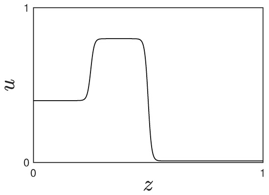
Figure 1. Initial condition $u(z,0)$ for problem (55) with a single overshoot.

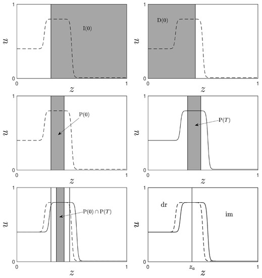
Figure 2. Schematic illustration for the decoupling of the imbibition and drainage fronts. The initial saturation profile $u(z,0)$ is the dashed line, and the propagated profile $u(z,T)$ with $T>0$ is shown as a solid line. The top left figure illustrates $\mathbb{I}\left(0\right)$ in gray, the top right figure illustrates $\mathbb{D}\left(0\right)$ in gray, the middle left figure shows the intersection $\mathbb{P}\left(0\right)=\mathbb{I}\left(0\right)\cap \mathbb{D}\left(0\right)$ at time $t=0$, the middle right figure shows $\mathbb{P}\left(T\right)$ at some time $T>0$, and the lower left figure shows $\mathbb{P}\left(0\right)\cap \mathbb{P}\left(T\right)$. The location $z_a$ in the lower right subfigure can be chosen arbitrarily from within the gray interval $\mathbb{P}\left(0\right)\cap \mathbb{P}\left(T\right)$ in the lower left subfigure.

Numerical solutions for problem (55) with initial data as shown in Figure 1 were studied in [6,7,8]. For this simple class of processes with a single saturation overshoot, the saturation history at positions $z>z_a$ has length $N\left(z\right)=0$, while $N\left(z\right)=1$ for $z\le z_a$. For any time t with $0<t<T$, there is a fixed graph ${\mathcal{G}}^{\mathrm{im}}$ describing the flow process at each $z\in \mathbb{I}\left(t\right)$ in terms of a flow function $f_{\mathrm{im}}(u;\left\{u_{\ast 0}\right\})$ parametrized by the saturation value $u_{\ast 0}=u(z,0)$ at $t^0=0$. Furthermore, there is a fixed graph ${\mathcal{G}}^{\mathrm{dr}}$ describing the flow process at each $z\in \mathbb{D}\left(t\right)$ in terms of a flow function $f_{\mathrm{dr}}(u;\left\{u_{\ast 1}\right\})$ parametrized by the saturation value $u_{\ast 1}=u(z,t^1)$ at the time instant $t^1\left(z\right)$ when the flow process switched from imbibition to drainage. For a single overshoot, the value of $u_{\ast 1}$ is, of course, $u_{\ast z}={max}_{z\in \mathsf{\Omega }}u(z,0)$. By continuity of the hysteresis model and by continuity of the graph $\mathcal{G}={\mathcal{G}}^{\mathrm{im}}\cup {\mathcal{G}}^{\mathrm{dr}}$, the flux is continous for all $z\in \mathbb{P}\left(t\right)$ with $0<t<T$. In this situation, the first order term in Equation (55) simplifies to

$$\begin{array}{}\hfill \frac{\partial }{\partial z}{f}_{{}_{\mathcal{G}}}\left(u\right)& =\frac{\partial }{\partial z}\left({\chi }_{\mathbb{I}\left(t\right)}{f}_{\mathrm{im}}(u;\left\{u_{\ast 0}\right\})+{\chi }_{\mathbb{D}\left(t\right)}{f}_{\mathrm{dr}}(u;\left\{u_{\ast 1}\right\})-{\chi }_{\mathbb{P}\left(t\right)}{f}_{\mathrm{im}}(u;\left\{u_{\ast 0}\right\})\right)\hfill & \mathrm{(57a)}\hfill & =\frac{\partial }{\partial z}\left({\chi }_{\mathbb{I}\left(t\right)}{f}_{\mathrm{im}}(u;\left\{u_{\ast 0}\right\})+{\chi }_{\mathbb{D}\left(t\right)}{f}_{\mathrm{dr}}(u;\left\{u_{\ast 1}\right\})-{\chi }_{\mathbb{P}\left(t\right)}{f}_{\mathrm{dr}}(u;\left\{u_{\ast 1}\right\})\right)\hfill & \mathrm{(57b)}\hfill & ={\chi }_{\mathbb{I}\left(t\right)}{f}_{\mathrm{im}}^{\prime }(u;\left\{u_{\ast 0}\right\})u_z+{\chi }_{\mathbb{D}\left(t\right)}{f}_{\mathrm{dr}}^{\prime }(u;\left\{u_{\ast 1}\right\})u_z-{\chi }_{\mathbb{P}\left(t\right)}{f}_{\mathrm{im}}^{\prime }(u;\left\{u_{\ast 0}\right\})u_z\hfill & \mathrm{(57c)}\hfill & =\chi (z,z_a)f_{\mathrm{im}}^{\prime }(u;\left\{u_{\ast 0}\right\})u_z+\left[1-\chi (z,z_a)\right]f_{\mathrm{dr}}^{\prime }(u;\left\{u_{\ast 1}\right\})u_z\hfill & \mathrm{(57d)}\end{array}$$

where $f_{\mathrm{im}}(·;\left\{u_{\ast 0}\right\})=f_{{\mathcal{G}}^{\mathrm{im}}}(·)$ and $f_{\mathrm{dr}}(·;\left\{u_{\ast 0}\right\})=f_{{\mathcal{G}}^{\mathrm{dr}}}(·)$. A possible choice for $f_{{}_{\mathcal{G}}}$ can be seen in ([8], Equation (2)). The term ${\chi }_{\mathbb{P}\left(t\right)}{f}_{\mathrm{im}}^{\prime }(u;\left\{u_{\ast 0}\right\})u_z$ is necessary because the imbibition interval and drainage interval are overlapping in the plateau interval $\mathbb{P}\left(t\right)$. Inserting this into the differential Equation (55) gives

$$u_t+\chi (z,z_a)f_{\mathrm{im}}^{\prime }(u;\left\{u_{\ast 0}\right\})u_z+\left[1-\chi (z,z_a)\right]f_{\mathrm{dr}}^{\prime }(u;\left\{u_{\ast 1}\right\})u_z-D{u}_{zz}=0$$

(58a)

where $\left\{u_{\ast 0}\right\}=u_0\left(z\right)=u(z,0)$ is the initial condition and $\left\{u_{\ast 1}\right\}=u(z,t^1\left(z\right))$ is the saturation at position z at the switching time $t^1$. The fractional flow functions for imbibition and drainage at the switching point obey flux continuity at $t^1$, i.e.

$$f_{\mathrm{im}}(u(z,t^1);\left\{u_{\ast 0}\right\})=f_{\mathrm{dr}}(u(z,t^1);\left\{u_{\ast 1}\right\})$$

(58b)

for all $z\in \mathbb{P}\left(t\right)$. Note that the fractional flow functions are explicitly position dependent due to hysteresis.

Numerical (and experimental) evidence in [6,7,8] suggest that imbibition and drainage fronts decouple for the simple class of hysteretic processes with a single saturation overshoot assumed in our mathematical model. The decoupling assumption is supported by noting that, for $D=0$, piecewise constant functions are indeed weak solutions.

The decoupling is implemented here in this work by assuming that the set $\mathbb{P}\left(t\right)$ has positive measure for some nonempty time interval $[0,T]$ with $T>0$. If the decoupling assumption holds true, then the fractional flow functions

$$f_{\mathrm{im}}(u(z,t);\left\{u_{\ast 0}\right\})=f_{\mathrm{dr}}(u(z,t);\left\{u_{\ast 1}\right\})$$

(59)

agree for all $z\in \mathbb{P}\left(t\right)$. In this way, a plateau in the saturation determines two position-independent fractional flow functions that agree on $\mathbb{P}\left(t\right)$ for $0<t<T$. The rigorous results for problem (1) obtained in this work support the numerical results for problem (55) in [8]. The main point here is that, given a non-monotone single overshoot initial condition similar to the one shown in Figure 1, there is an open interval ${\bigcap }_{t=0}^T\mathbb{P}\left(t\right)\subset (\mathbb{I}\left(t\right)\cap \mathbb{D}\left(t\right))$ with $u=const.$ for $t\in [0,T]$ and $z_a\in {\bigcap }_{t=0}^T\mathbb{P}\left(t\right)$. This fact ensures the decoupling of the imbibition and the drainage front, and Equation (55) can be reduced to Equation (1) for $t\in [0,T]$.

References

- Alt, H.W.; Luckhaus, S.; Visintin, A. On nonstationary flow through porous media. Ann. Di Mat. Pura Ed Appl. 1985, 136, 303–316. [Google Scholar] [CrossRef]
- Amadori, D.; Baiti, P.; Corli, A.; Dal Santo, E. Global weak solutions for a model of two-phase flow with a single interface. J. Evol. Equations 2015, 15, 699–726. [Google Scholar] [CrossRef] [Green Version]
- Cao, X.; Pop, I.S. Two-phase porous media flows with dynamic capillary effects and hysteresis: Uniqueness of weak solutions. Comput. Math. Appl. 2015, 69, 688–695. [Google Scholar] [CrossRef]
- Cao, X.; Pop, I.S. Degenerate two-phase porous media flow model with dynamic capillarity. J. Differ. Equations 2016, 260, 2418–2456. [Google Scholar] [CrossRef]
- Mikelić, A. A global existence result for the equations describing unsaturated flow in porous media with dynamic capillary pressure. J. Differ. Equations 2010, 248, 1561–1577. [Google Scholar] [CrossRef] [Green Version]
- Hilfer, R.; Steinle, R. Saturation overshoot and hysteresis for twophase flow in porous media. Eur. Phys. J. Spec. Top. 2014, 223, 2323–2338. [Google Scholar] [CrossRef]
- Steinle, R.; Hilfer, R. Influence of initial conditions on propagation, growth and decay of saturation overshoot. Transp. Porous Media 2016, 111, 369–380. [Google Scholar] [CrossRef]
- Steinle, R.; Hilfer, R. Hysteresis in relative permeabilities suffices for propagation of saturation overshoot: A quantitative comparison with experiment. Phys. Rev. E 2017, 95, 043112–1–043112–10. [Google Scholar] [CrossRef] [PubMed] [Green Version]
- Böhm, M.; Showalter, R.E. A nonlinear pseudoparabolic diffusion equation. SIAM J. Math. Anal. 1985, 16, 980–999. [Google Scholar] [CrossRef]
- Cuesta, C.; Hulshof, J. A model problem for groundwater flow with dynamic capillary pressure: Stability of travelling waves. Nonlinear Anal. 2003, 52, 1199–1218. [Google Scholar] [CrossRef]
- Hulshof, J.; King, J.R. Analysis of a Darcy flow model with a dynamic pressure saturation relation. SIAM J. Appl. Math. 1999, 59, 318–346. [Google Scholar]
- Köhne, M.; Prüss, J.; Wilke, M. On quasilinear parabolic evolution equations in weighted Lp-spaces. J. Evol. Equations 2010, 10, 443–463. [Google Scholar] [CrossRef] [Green Version]
- Kopfová, J. Nonlinear semigroup methods in problems with hysteresis. Discret. Contin. Dyn. Syst. Suppl. 2007, 2007, 580–589. [Google Scholar]
- Pazy, A. Semigroups of Linear Operators and Applications to Partial Differential Equations; Springer: Berlin/Heidelberg, Germany, 1983. [Google Scholar]
- Yagi, A. Abstract Parabolic Equations and Their Applications; Springer: Berlin/Heidelberg, Germany, 2010. [Google Scholar]
- Little, T.D.; Showalter, R.E. Semilinear Parabolic Equations With Preisach Hysteresis. Differ. Integral Equations 1994, 7, 1021–1040. [Google Scholar]
- Zeidler, E. Nonlinear Functional Analysis and its Applications I: Fixed-Point Theorems; Springer: New York, NY, USA, 1986. [Google Scholar]
Publisher’s Note: MDPI stays neutral with regard to jurisdictional claims in published maps and institutional affiliations. |
© 2022 by the authors. Licensee MDPI, Basel, Switzerland. This article is an open access article distributed under the terms and conditions of the Creative Commons Attribution (CC BY) license (https://creativecommons.org/licenses/by/4.0/).