Article

A Reliable Combination of Double Laplace Transform and Homotopy Analysis Method for Solving a Singular Nonlocal Problem with Bessel Operator

Department of Mathematics, College of Science, King Saud University, Riyadh 11451, Saudi Arabia
*
Author to whom correspondence should be addressed.
Axioms 2023, 12(10), 933; https://doi.org/10.3390/axioms12100933
Submission received: 31 August 2023 / Revised: 22 September 2023 / Accepted: 28 September 2023 / Published: 29 September 2023
(This article belongs to the Special Issue The Numerical Analysis and Its Application)

Abstract

:
In this article, we present a numerical iterative scheme for solving a non-local singular initial-boundary value problem by combining two well known efficient methods. Namely, the homotopy analysis method and the double Laplace transform method. The resulting scheme is tested on a set of test examples to illustrate its efficiency, it generates the exact analytical solution for each one of these examples. The convergence of the resulting numerical solutions of these examples is tested both graphically and numerically.

1. Introduction

Many applications in engineering and natural sciences involve mathematical models with nonclassical conditions. Usually these models involve initial-boundary value problems accompanied with constraints of integral type. These models appear in various applications such as thermoelasticity, transmission theory, chemical diffusion, control theory, nuclear reactor dynamics, etc. See for example Muravei and Philinovskii [1], Nakhushev [2], Pulkina [3,4], Samarskii [5], Shi and Shillor [6], Cannon [7], Ionkin and Moiseev [8], Kacur and Keer [9].
Unfortunately, theoretical analytical solutions of this type of problems mostly can not be determined, especially for nonlinear problems. Thus, in the literature various numerical techniques have been developed by several researchers to determine approximate solutions for these problems. In [10], finite difference methods have been used to address a one-dimensional parabolic partial differential equation with initial and nonlocal boundary conditions that involve nonlocal integral terms. Meanwhile, a combination of finite difference and orthogonal function approximation techniques has been utilized to solve a one-dimensional parabolic equation featuring two integral conditions, as demonstrated in [11]. Furthermore, a hybrid approach integrating finite difference and spectral methods has been proposed for solving a one-dimensional wave equation accompanied with an integral condition, as presented in [12]. Moreover, the Chebyshev spectral method is used to solve a class of local and nonlocal elliptic boundary value problems in [13]. Also, the finite element method is employed to solve a nonlocal problem of Kirchhoff type in [14].
On the other hand, several computational techniques that do not require discretization have been developed in the last decades. For example the differential transform method is applied in [15,16]. The Adomian decomposition method given in [17,18,19], which is developed to treat nonlinearity in partial differential equations. In addition to that Laplace decomposition method is given in [20,21]. One more analytical method is the variational iteration method given in [22,23]. Another method is the homotopy perturbation presented in [24,25,26]. A powerful analytical technique which is widely used by many researchers is the homotopy analysis method introduced by Liao [27,28,29,30,31].
In this work, we combined two well known techniques, the homotopy analysis method and the double Laplace transform method, to develop a numerical scheme, named as homotopy analysis double Laplace transform method (HADLTM), to solve a singular one-dimensional parabolic equation subject to Dirichlet conditions and a non-local condition of integral type. To our knowledge it is the first time in the literature where such combination between these two methods is applied.
Here we will consider the following problem:
L η ( x , t ) = G ( x , t ) , ( x , t ) Ω = ( 0 , 1 ) × [ 0 , T ] , η ( x , t ) : = η ( x , 0 ) = w ( x ) , x ( 0 , 1 ) , 0 1 x η ( x , t ) d x = 0 , η ( 1 , t ) = 0 , t ( 0 , T ) ,
where L is the operator t 1 x x x x , and G and w ( x ) are known functions.
Problem (1) can be written in an operator form as:
K η = ( L , ) η = : F ,
in which K is an unbounded operator that satisfies K : A H , with domain all functions of η in the set:
D ( ( Ω ) = { η : η , η t , η x , a n d η x x L x 2 ( Ω ) }
which satisfy the given boundary conditions, and A is a Banach space of functions η equipped with a finite norm as [32]:
η A 2 = η t L x 2 ( Ω ) 2 + x ( x η x ) L x 2 ( Ω ) 2 + sup 0 τ T η ( x , τ ) W x 1 ( Ω ) 2 ,
with values in the Hilbert space H consisting of the functions F = ( G , w ) L x 2 ( Ω ) × W x 1 ( Ω ) equipped with the norm [32]:
F H 2 = G L x 2 ( Ω ) 2 + w W x 1 ( Ω ) 2 .
The double Laplace transform of a function f ( x , t ) is given as [33,34,35]:
L x L t f ( x , t ) = 0 e r x 0 e s t f ( x , t ) d t d x = : F ( r , s ) ,
where x and t are positive real variables, and r and s are complex variables. On the other hand, the double Laplace transform of its time-partial derivative; f t ( x , t ) , is given by:
L x L t f ( x , t ) t = s F ( r , s ) F ( r , 0 ) ,
where F is the double Laplace transform of f.
The rest of the article is organized as follows: In Section 2, we recall some existence results of the solution of problem (1). In Section 3, we present the development of the numerical scheme for solving problem (1) based on the HADLTM. In Section 4, we provide several examples to test the applicability and efficiency of the developed scheme. Finally, we present some comments and conclusions in Section 5.

2. Existence and Uniqueness of the Solution

Here, we present some existence and uniqueness results of the solution of problem (1). First, we recall the two sided a prior estimates:
Theorem 1
([32,36]). For every function η D ( K ) , we have:
K η H 2 2 η A ,
Theorem 2
([32,36]). For every function η D ( K ) , the following energy inequality holds true:
η A C K η H ,
for some positive constant C independent of η.
As pointed in it [32], in view of Theorem 1, it follows that the operator K : A H is continuous. Thus, Theorem 2 implies that the set R ( K ) H ; the range of K , is closed. Hence, the inverse operator K 1 exists and is continuous. To verify the existence of the solution of (1), we need to verify that the set I m ( K ) ; the image of K , coincides with the whole Hilbert space H .
Theorem 3
([32,36]). For any two functions G L x 2 ( Ω ) and w W x 1 ( Ω ) , there exists a unique solution η = K 1 Ψ of problem (1) that satisfies the inequality
η A C K η H ,
where Ψ = ( G , w ) , and C is a positive constant which does not depend on η.

3. Method Development

Consider a general partial differential equation as:
θ t + R ˜ θ ( x , t ) + N ˜ θ ( x , t ) = f ( x , t ) ,
where θ is an unknown function in x and t, R ˜ is a linear differential operator, N ˜ represents a nonlinear differential operator, and f is a given function. Applying double Laplace transform on both sides of (3), implies:
s Θ ( r , s ) Θ ( r , 0 ) + L x L t R ˜ θ ( x , t ) + N ˜ θ ( x , t ) = L x L t f ( x , t ) ,
or equivalently,
Θ ( r , s ) 1 s Θ ( r , 0 ) + 1 s L x L t R ˜ θ ( x , t ) + N ˜ θ ( x , t ) f ( x , t ) = 0 ,
where Θ ( r , s ) is the double Laplace transform of θ ( x , t ) . According to the homotopy analysis method [27], we define the operator:
N [ ϕ ( x , t ; p ) ] = L x L t ϕ ( x , t ; p ) 1 s Θ ( r , 0 ) + 1 s L x L t R ˜ ϕ ( x , t ; p ) + N ˜ ϕ ( x , t ; p ) f ( x , t ) ,
where p [ 0 , 1 ] , and ϕ is a real valued function of x , t and p. Thus, the zeroth-order deformation equation will be on the form:
( 1 p ) L x L t ϕ ( x , t ; p ) θ 0 ( x , t ) = p N [ ϕ ( x , t ; p ) ] ,
where 0 is an auxiliary parameter, p [ 0 , 1 ] is an embedding parameter, θ 0 ( x , t ) is an initial guess to start with to get the solution θ ( x , t ) , and ϕ ( x , t ; p ) is an unknown function.
In view of Equation (4), it is clear that for p = 0 and p = 1 we obtain:
ϕ ( x , t ; 0 ) = θ 0 ( x , t ) and ϕ ( x , t ; 1 ) = θ ( x , t ) .
Thus, as p increases from 0 to 1, the function ϕ ( x , t ; p ) deforms from θ 0 ( x , t ) to the exact solution θ ( x , t ) .
Then, using the Taylor series expansion of ϕ ( x , t ; p ) with respect to p gives:
ϕ ( x , t ; p ) = θ 0 ( x , t ) + k = 1 θ k ( x , t ) p k ,
where
θ k ( x , t ) = 1 k ! k ϕ ( x , t ; p ) p k p = 0 .
As Liao mentioned in [30] if the auxiliary parameter , the inverted operator L , and the initial guess θ 0 ( x , t ) are chosen properly, then the power series (5) will converge at p = 1 to one of the solutions of the original equation, and this solution is given in a series form as:
θ ( x , t ) = θ 0 ( x , t ) + k = 1 θ k ( x , t ) ,
as pointed out by Liao in [28], the parameter helps one in controlling and adjusting the convergence region of the series solution. The values of this parameter can be determined through the curve.
Now, differentiating Equation (4) k-times with respect to p, dividing by k ! , then setting p = 0 , produces the kth order deformation equations as:
L x L t θ k ( x , t ) χ k θ k 1 ( x , t ) = R ( θ k 1 ) ,
where
θ k ( x , t ) = [ θ 0 ( x , t ) , θ 1 ( x , t ) , , θ k ( x , t ) ] ,
and
R ( θ k 1 ) = 1 ( k 1 ) ! k 1 p k 1 N ϕ ( x , t ; p ) p = 0 .
Then, applying the inverse double Laplace transform to both sides of (6), the components θ k ( x , t ) of the HADLTM can be determined recursively through the formula:
θ k ( x , t ) = χ k θ k 1 ( x , t ) + L r 1 L s 1 R ( θ k 1 ) ,
where
χ k = 0 , k 1 , 1 , k > 1 .

4. Application of the Method

The presence of the integral condition in problem (1) complicates the computations. Therefore, to avoid this difficulty in exploring the applicability and efficiency of the HADLTM for solving this problem, we consider the forthcoming equivalent problem (9), in which the integral condition is replaced by classical conditions.
Thus, suppose that 0 1 x θ ( x , t ) d x = 0 and 0 1 x f ( x , t ) d x = 0 . Then, multiplying the equation:
t θ ( x , t ) 1 x x θ ( x , t ) 2 x 2 θ ( x , t ) = f ( x , t ) ,
by x, and integrating the resulting equation with respect to x on the interval [ 0 , 1 ] , gives:
t 0 1 x θ ( x , t ) d x 0 1 θ x ( x , t ) d x 0 1 x θ x x ( x , t ) d x = 0 1 x f ( x , t ) d x ,
or
t 0 1 x θ ( x , t ) d x 0 1 θ x ( x , t ) d x x θ x ( x , t ) 0 1 0 1 θ x ( x , t ) = 0 1 x f ( x , t ) d x ,
which implies θ x ( 1 , t ) = 0 .
Conversely, suppose that θ x ( 1 , t ) = 0 , and 0 1 x f ( x , t ) d x = 0 . Now, multiplying Equation (7) by x, and integrating the resulting equation with respect to x on [ 0 , 1 ] , then using (8), we get t 0 1 x θ ( x , t ) d x = 0 , which implies 0 1 x θ ( x , t ) d x = c , t [ 0 , 1 ] , where c is a constant.
In particular 0 1 x θ ( x , 0 ) d x = c = 0 , as the initial condition θ ( x , 0 ) = η ( x ) satisfies the compatibility condition, which implies 0 1 x θ ( x , t ) d x = 0 .
Therefore the condition 0 1 x θ ( x , t ) d x = 0 in problem (1) is equivalent to the conditions θ x ( 1 , t ) = 0 and 0 1 x f ( x , t ) d x = 0 . Thus, problem (1) is equivalent to:
θ ( x , t ) t 1 x x x θ ( x , t ) x = f ( x , t ) , 0 < x < 1 , 0 < t < T , θ ( x , 0 ) = η ( x ) , 0 < x < 1 , θ ( 1 , t ) = φ ( t ) , θ x ( 1 , t ) = 0 , t ( 0 , T ) ,
provided that 0 1 x f ( x , t ) d x = 0 , where f , η and φ are given functions.
Now, in view of (2), taking double Laplace transform for both sides of (9), we obtain:
Θ ( r , s ) 1 s Θ ( r , 0 ) 1 s L x L t 1 x x x θ ( x , t ) x + f ( x , t ) = 0 .
Thus, we define the operator N [ ϕ ( x , t ; q ) ] as:
N [ ϕ ( x , t ; p ) ] = L x L t ϕ ( x , t ; p ) 1 s Θ ( r , 0 ) 1 s L x L t 1 x x x ϕ ( x , t ; p ) x + f ( x , t ) .
Hence, the kth order deformation equation is given by:
L x L t [ θ k ( x , t ) χ k θ k 1 ( x , t ) ] = R ( θ k 1 ) ,
where
R ( θ k 1 ) = L x L t θ k 1 ( x , t ) 1 χ k 1 s Θ ( r , 0 ) 1 s L x L t 1 x x x θ k 1 ( x , t ) x + 1 χ k f ( x , t ) .
Hence, the series solution is given as:
θ ( x , t ) = θ 0 ( x , t ) + k = 1 θ k ( x , t ) .
where
θ k ( x , t ) = χ k θ k 1 ( x , t ) + L r 1 L s 1 R ( θ k 1 ) .
To test the efficiency of the scheme (10) in handling the numerical solutions of problems of the type (9), it is applied to the forthcoming set of test examples.
Example 1.
Consider the homogeneous PDE:
θ ( x , t ) t 1 x θ ( x , t ) x 2 θ ( x , t ) x 2 = 0 , 0 < x < 1 , 0 < t < T ,
satisfying the following initial and boundary conditions:
θ ( x , 0 ) = x 2 4 ln ( x ) 2 , 0 < x < 1 , θ ( 1 , t ) = t + 1 4 , θ x ( 1 , t ) = 0 , 0 < t < T .
Solution.
Let θ 0 ( x , t ) = θ ( x , 0 ) = x 2 4 ln ( x ) 2 + 1 2 . In view of (10) we obtain:
θ 1 ( x , t ) = χ 1 θ 0 ( x , t ) + L r 1 L s 1 [ R ( θ 0 ) ] = L r 1 L s 1 [ R ( θ 0 ) ] = L r 1 L s 1 L x L t { θ 0 ( x , t ) } ( 1 χ 1 ) 1 s Θ ( r , 0 ) 1 s L x L t { 1 x ( θ 0 ( x , t ) ) x + ( θ 0 ( x , t ) ) x x } = L r 1 L s 1 L x L t { θ 0 ( x , t ) } ( 1 χ 1 ) 1 s Θ ( r , 0 ) 1 s L x L t { 1 } = t .
θ 2 ( x , t ) = χ 2 θ 1 ( x , t ) + L r 1 L s 1 [ R ( θ 1 ) ] = θ 1 ( x , t ) + L r 1 L s 1 [ R ( θ 1 ) ] = θ 1 ( x , t ) + L r 1 L s 1 L x L t { θ 1 ( x , t ) } = ( 1 + ) θ 1 ( x , t ) .
θ 3 ( x , t ) = χ 3 θ 2 ( x , t ) + L r 1 L s 1 [ R ( θ 2 ) ] = θ 2 ( x , t ) + L r 1 L s 1 [ R ( θ 2 ) ] = θ 2 ( x , t ) + L r 1 L s 1 L x L t { θ 2 ( x , t ) } = ( 1 + ) θ 2 ( x , t ) = ( 1 + ) 2 θ 1 ( x , t )
In general we obtain:
θ j ( x , t ) = ( 1 + ) j 1 θ 1 ( x , t ) , j 1 ,
hence, we have:
θ ( x , t ) = θ 0 ( x , t ) + j = 1 θ j ( x , t ) = θ 0 ( x , t ) j = 1 ( 1 + ) j 1 t .
Now, if we choose the parameter within the range 2 < < 0 , then the series (11) converges to the exact solution given by:
θ ( x , t ) = θ 0 ( x , t ) + t = x 2 4 ln ( x ) 2 + t .
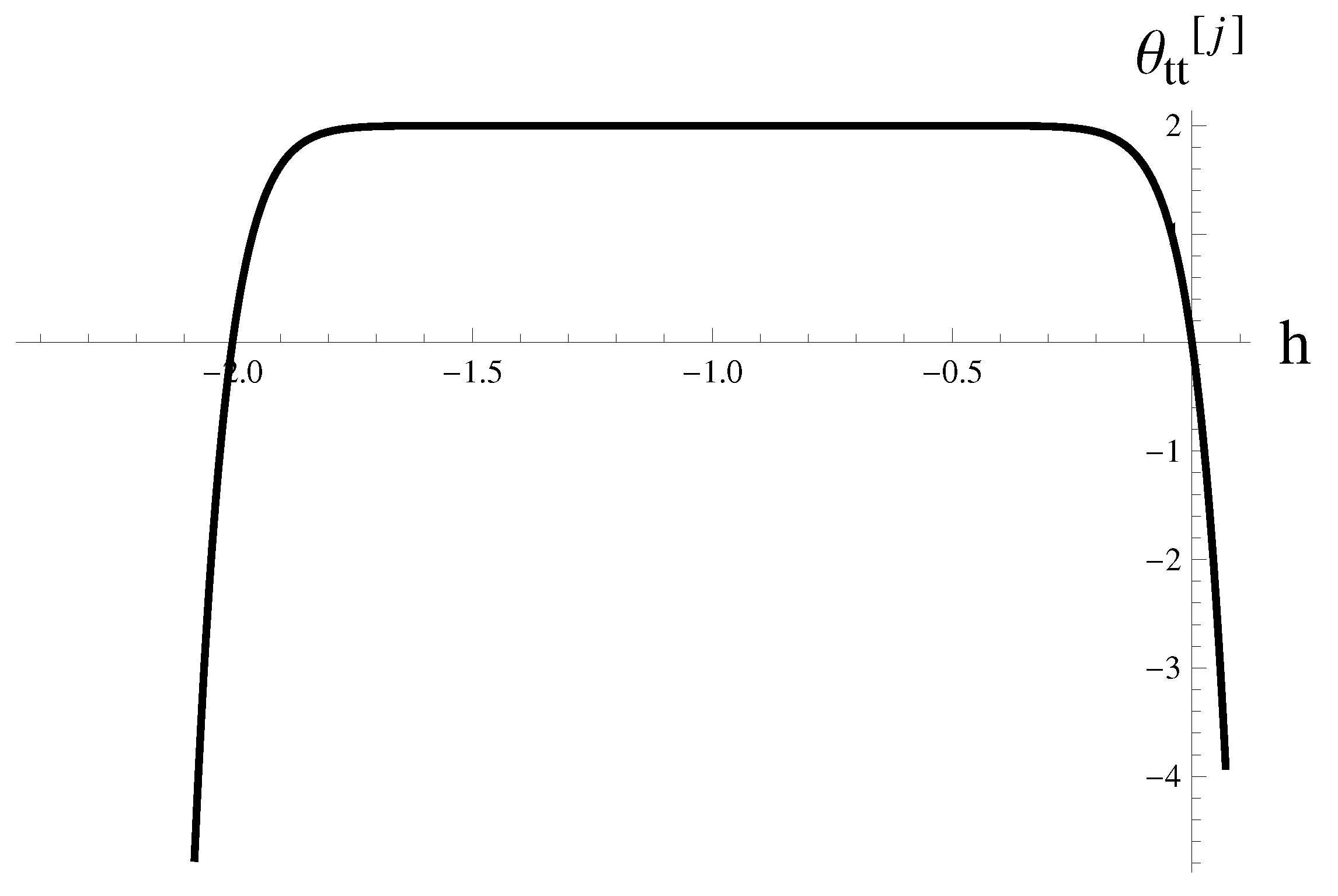
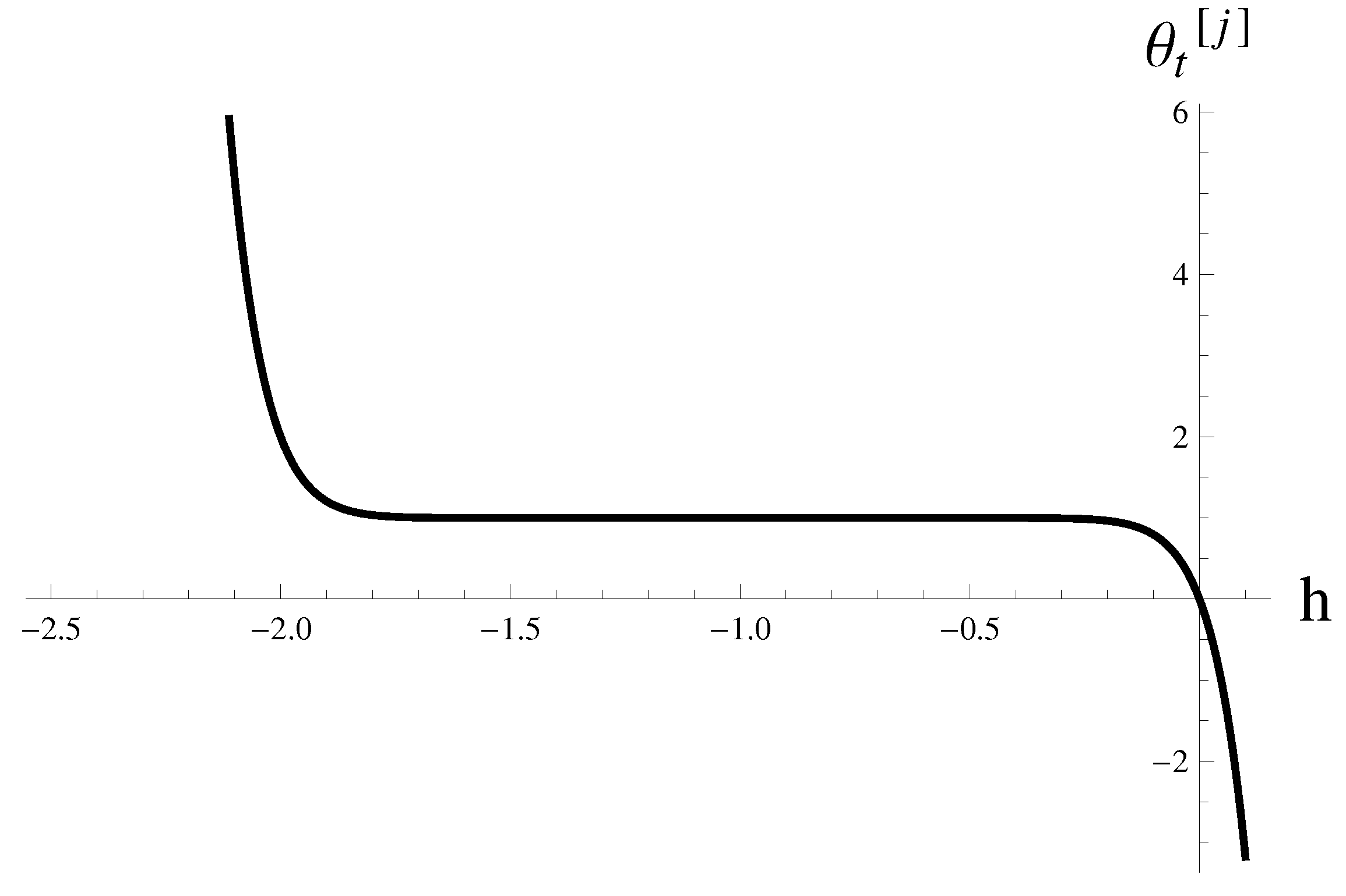
Figure 1 displays the h-curve corresponding to the 15th order truncated series solution at x = 0.75 , from which it appears that the values of the parameter required for the convergence of the series solution are located in the interval 1.8 < < 0.2 .
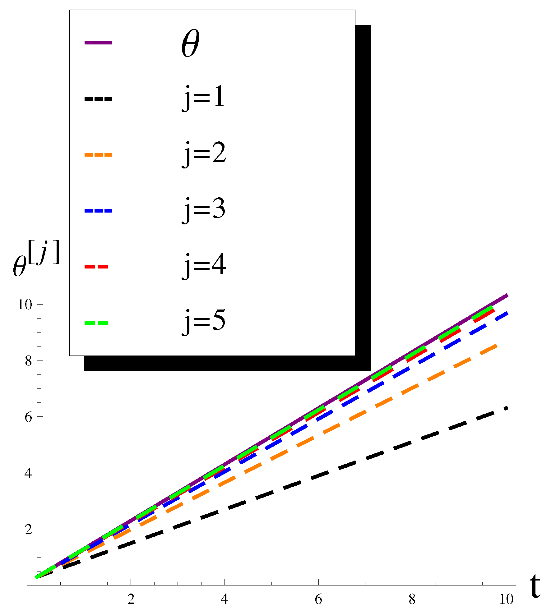
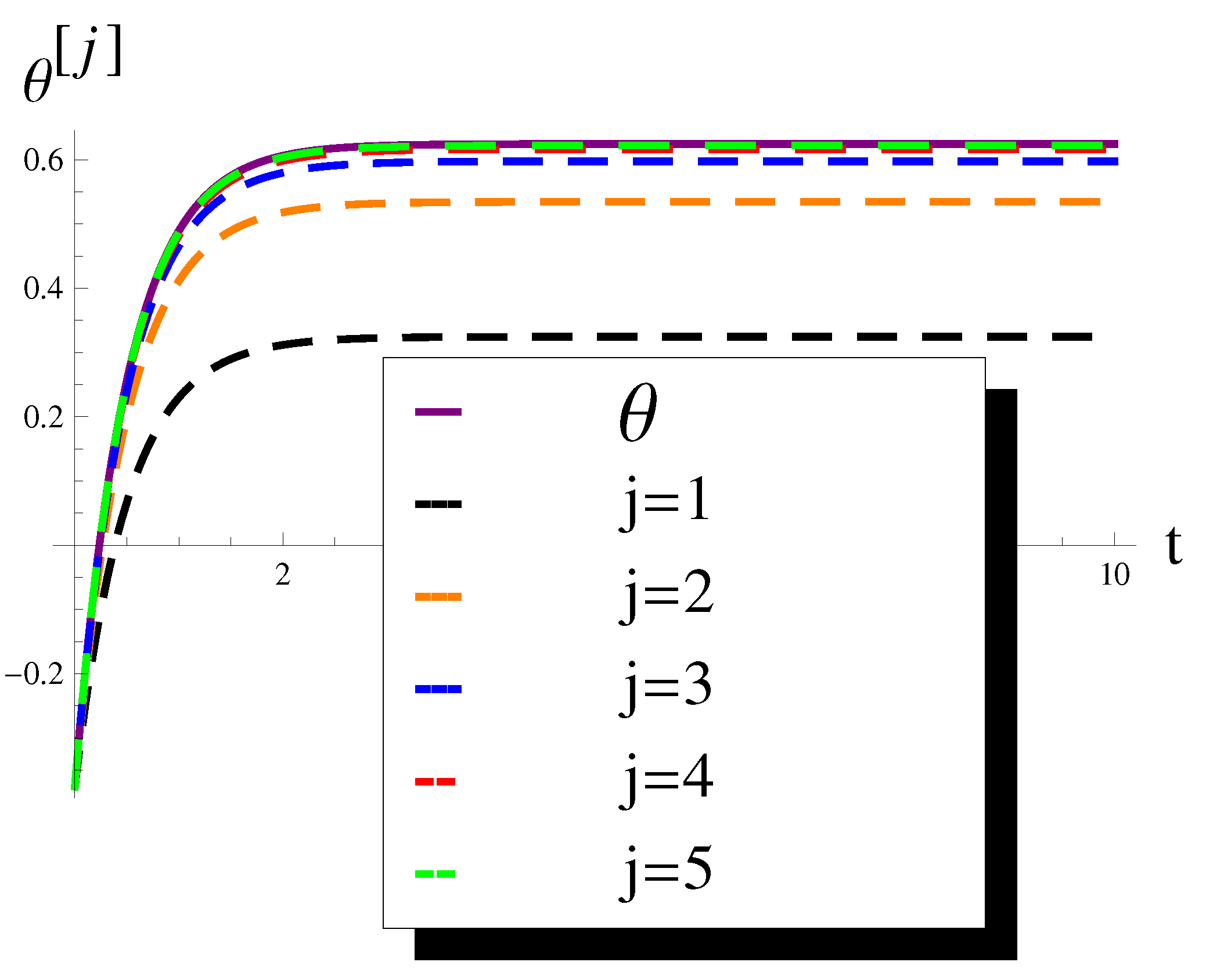
Figure 2 shows the plots of the truncated series solution using different number of terms together with the corresponding exact solution of Example 1 at x = 0.7 and = 0.6 . It shows that the truncated series solution of order j = 5 is very close to the exact solution, which shows the rapid convergence of the proposed method.
Table 1 shows the absolute error E r [ j ] = | θ ( x , t ) θ [ j ] ( x , t ) | due to the difference between the exact solution and the approximate solution of distinct orders of Example 1 at different values of x and t. It illustrates the rapid convergence of the approximate solution obtained by using this method.
Example 2.
Consider the nonhomogeneous PDE:
θ ( x , t ) t 1 x θ ( x , t ) x 2 θ ( x , t ) x 2 = 2 t + 4 x 2 , 0 < x < 1 , 0 < t < T ,
subject to the conditions:
θ ( x , 0 ) = ln ( x ) x 4 4 , 0 < x < 1 , θ ( 1 , t ) = t 2 1 4 , θ x ( 1 , t ) = 0 , 0 < t < T .
Solution.
Let θ 0 ( x , t ) = θ ( x , 0 ) = 1 + x 4 4 ln ( x ) . Then, in view of (10) we get:
θ 1 ( x , t ) = χ 1 θ 0 ( x , t ) + L r 1 L s 1 [ R ( θ 0 ) ] = L r 1 L s 1 [ R ( θ 0 ) ] = L r 1 L s 1 L x L t { θ 0 ( x , t ) } ( 1 χ 1 ) 1 s Θ ( r , 0 ) 1 s L x L t { 1 x ( θ 0 ( x , t ) ) x + ( θ 0 ( x , t ) ) x x } = L r 1 L s 1 L x L t { θ 0 ( x , t ) } ( 1 χ 1 ) 1 s Θ ( r , 0 ) 1 s L x L t { 4 x 2 } = t 2 .
θ 2 ( x , t ) = χ 2 θ 1 ( x , t ) + L r 1 L s 1 [ R ( θ 1 ) ] = θ 1 ( x , t ) + L r 1 L s 1 [ R ( θ 1 ) ] = θ 1 ( x , t ) + L r 1 L s 1 L x L t { θ 1 ( x , t ) } = ( 1 + ) θ 1 ( x , t ) .
θ 3 ( x , t ) = χ 3 θ 2 ( x , t ) + L r 1 L s 1 [ R ( θ 2 ) ] = θ 2 ( x , t ) + L r 1 L s 1 [ R ( θ 2 ) ] = θ 2 ( x , t ) + L r 1 L s 1 L x L t { θ 2 ( x , t ) } = ( 1 + ) θ 2 ( x , t ) = ( 1 + ) 2 θ 1 ( x , t )
Proceeding on this manner we obtain:
θ j ( x , t ) = ( 1 + ) j 1 θ 1 ( x , t ) , j 1 ,
hence, we have:
θ ( x , t ) = θ 0 ( x , t ) + j = 1 θ j ( x , t ) . = θ 0 ( x , t ) j = 1 ( 1 + ) j 1 t 2 .
Hence, if the parameter satisfies 2 < < 0 , then the series (12) converges to the exact solution given by:
θ ( x , t ) = θ 0 ( x , t ) + t 2 = ln ( x ) x 4 4 + t 2 .
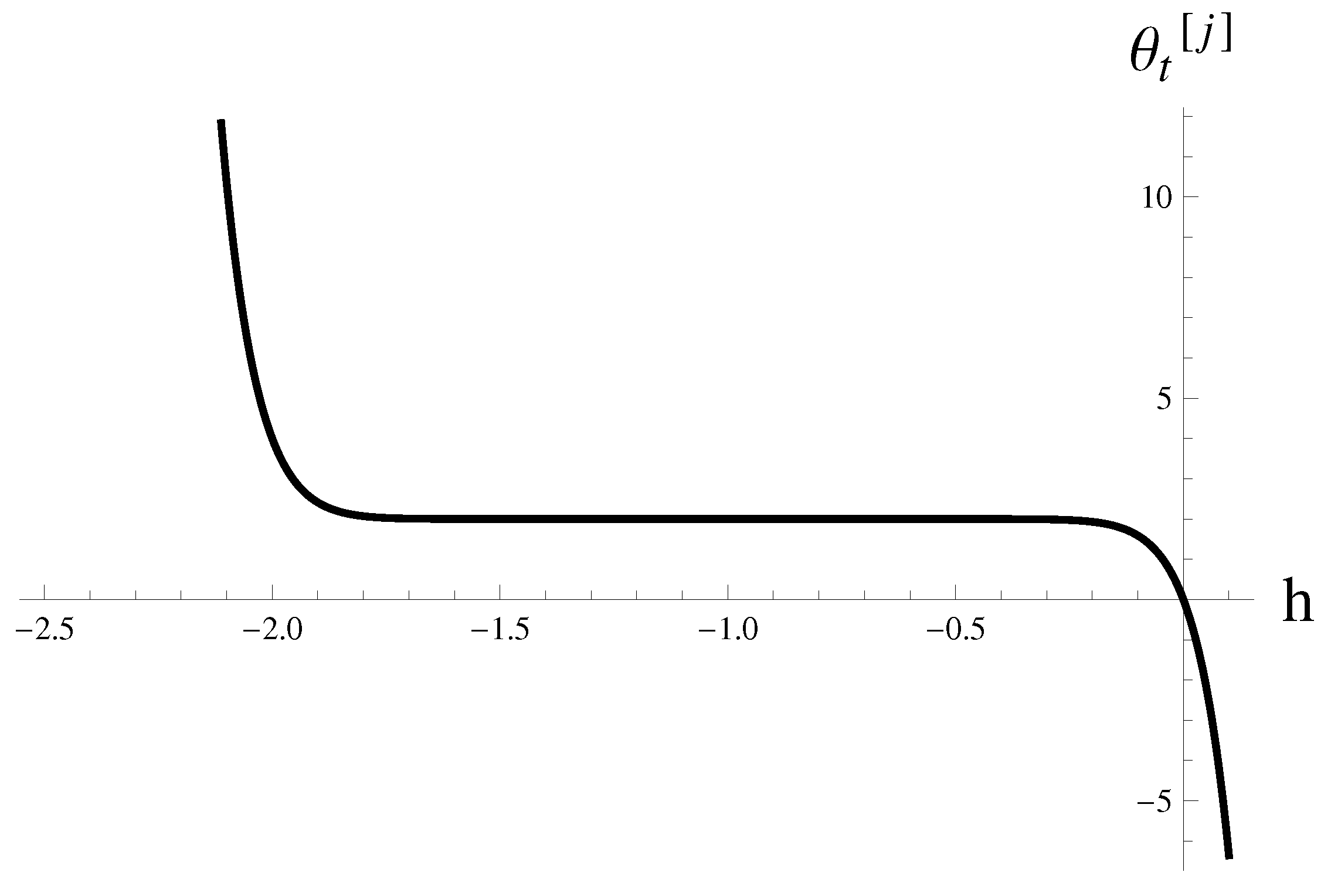
Figure 3 shows the h-curve corresponding to the 16th order truncated series solution at x = 0.75 , it appears that the valid values of the parameter that lead to a convergent series solution are located in the interval 1.8 < < 0.2 .
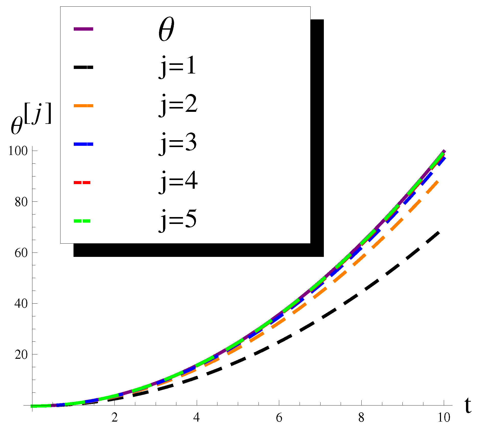
Figure 4 shows plots of the truncated series solution using different number of terms together with the corresponding exact solution of Example 2 at x = 0.8 and = 0.7 . It shows that the truncated series solution of order j = 5 almost coincide with the exact solution, which shows the rapid convergence of the proposed method.
Table 2 shows the absolute error E r [ j ] = | θ ( x , t ) θ [ j ] ( x , t ) | due to the difference between the exact solution and the approximate solution of distinct orders of Example 2 at different values of x and t. It illustrates the rapid convergence of the approximate solutions generated by this method.
Example 3.
Consider the nonhomogeneous PDE:
θ ( x , t ) t 1 x θ ( x , t ) x 2 θ ( x , t ) x 2 = 2 e 2 t 1 , 0 < x < 1 , 0 < t < T ,
subject to the constraints:
θ ( x , 0 ) = x 2 4 ln ( x ) 2 1 , 0 < x < 1 , θ ( 1 , t ) = 1 4 e 2 t , u x ( 1 , t ) = 0 , 0 < t < T ,
Solution.
Starting with θ 0 ( x , t ) = θ ( x , 0 ) = x 2 4 ln ( x ) 2 1 , in view of (10), we obtain:
θ 1 ( x , t ) = χ 1 θ 0 ( x , t ) + L r 1 L s 1 [ R ( θ 0 ) ] = L r 1 L s 1 [ R ( θ 0 ) ] = L r 1 L s 1 L x L t { θ 0 ( x , t ) } ( 1 χ 1 ) 1 s Θ ( r , 0 ) 1 s L x L t { 1 x ( θ 0 ( x , t ) ) x + ( θ 0 ( x , t ) ) x x } = L r 1 L s 1 L x L t { θ 0 ( x , t ) } ( 1 χ 1 ) 1 s Θ ( r , 0 ) 1 s L x L t { 1 } = ( e 2 t 1 ) .
θ 2 ( x , t ) = χ 2 θ 1 ( x , t ) + L r 1 L s 1 [ R ( θ 1 ) ] = θ 1 ( x , t ) + L r 1 L s 1 [ R ( θ 1 ) ] = θ 1 ( x , t ) + L r 1 L s 1 L x L t { θ 1 ( x , t ) } = ( 1 + ) θ 1 ( x , t ) .
θ 3 ( x , t ) = χ 3 θ 2 ( x , t ) + L r 1 L s 1 [ R ( θ 2 ) ] = θ 2 ( x , t ) + L r 1 L s 1 [ R ( θ 2 ) ] = θ 2 ( x , t ) + L r 1 L s 1 L x L t { θ 2 ( x , t ) } = ( 1 + ) θ 2 ( x , t ) = ( 1 + ) 2 θ 1 ( x , t ) .
In general we get:
θ j ( x , t ) = ( 1 + ) j 1 θ 1 ( x , t ) , j 1 ,
hence, the series solution takes the form:
θ ( x , t ) = θ 0 ( x , t ) + j = 1 θ j ( x , t ) . = θ 0 ( x , t ) + j = 1 ( 1 + ) j 1 ( e 2 t 1 ) .
Thus, if the parameter satisfies 2 < < 0 , then the series (12) converges to the exact solution:
θ ( x , t ) = θ 0 ( x , t ) + 1 e 2 t = x 2 4 ln ( x ) 2 e 2 t .
Figure 5 shows the h-curve corresponding to the 15th order truncated series solution at x = 0.7 , from which it appears that the valid values of the parameter that lead to a convergent series solution are located in the interval 1.8 < < 0.2 .
Figure 6 shows the plots of the truncated series solution using different number of terms together with the corresponding exact solution of Example 3 at x = 0.3 and = 0.7 . It shows that the truncated series solution of order j = 5 is very close to the exact solution, which demonstrates the rapid convergence of the proposed method.
Table 3 presents the absolute error E r [ j ] = | θ ( x , t ) θ [ j ] ( x , t ) | due to the difference between the exact solution and the approximate solution of distinct orders of Example 3 at different values of x and t. It illustrates the rapid convergence of the approximate solutions generated by this method.
Example 4.
Consider the nonhomogeneous PDE:
θ ( x , t ) t 1 x θ ( x , t ) x 2 θ ( x , t ) x 2 = cos ( t ) 2 , 0 < x < 1 , 0 < t < T ,
subject to the constraints:
θ ( x , 0 ) = x 2 2 ln ( x ) , 0 < x < 1 , θ ( 1 , t ) = sin ( t ) + 1 2 , u x ( 1 , t ) = 0 , 0 < t < T .
Solution.
Choosing θ 0 ( x , t ) = θ ( x , 0 ) = x 2 2 ln ( x ) , in view of (10), we have:
θ 1 ( x , t ) = χ 1 θ 0 ( x , t ) + L r 1 L s 1 [ R ( θ 0 ) ] = L r 1 L s 1 [ R ( θ 0 ) ] = L r 1 L s 1 [ L x L t { θ 0 ( x , t ) } 1 s Θ ( r , 0 ) 1 s L x L t { 1 x ( θ 0 ( x , t ) ) x + ( θ 0 ( x , t ) ) x x + ( 1 χ 1 ) ( cos ( t ) 2 ) } ] = L r 1 L s 1 L x L t { θ 0 ( x , t ) } 1 s Θ ( r , 0 ) 1 s L x L t { cos ( t ) } = L r 1 L s 1 L x L t { θ 0 ( x , t ) } 1 s Θ ( r , 0 ) 1 r ( s 2 + 1 ) = sin ( t ) .
θ 2 ( x , t ) = χ 2 θ 1 ( x , t ) + L r 1 L s 1 [ R ( θ 1 ) ] = θ 1 ( x , t ) + L r 1 L s 1 [ R ( θ 1 ) ] = θ 1 ( x , t ) + L r 1 L s 1 L x L t { θ 1 ( x , t ) } = ( 1 + ) θ 1 ( x , t ) .
Proceeding on this manner we get:
θ j ( x , t ) = ( 1 + ) j 1 θ 1 ( x , t ) ,
hence, the series solution is given as:
θ ( x , t ) = θ 0 ( x , t ) + j = 1 θ j ( x , t ) = θ 0 ( x , t ) j = 1 ( 1 + ) j 1 sin ( t ) .
It follows that if the parameter lies in the range 2 < < 0 , then the series (14) converges to the analytical solution:
θ ( x , t ) = θ 0 ( x , t ) + sin ( t ) = sin ( t ) + x 2 2 ln ( x ) ,
Figure 7 shows the h-curve corresponding to the 15th order truncated series solution at x = 0.7 , it appears that the valid values of the parameter that lead to a convergent series solution are located in the interval 1.8 < < 0.2 .
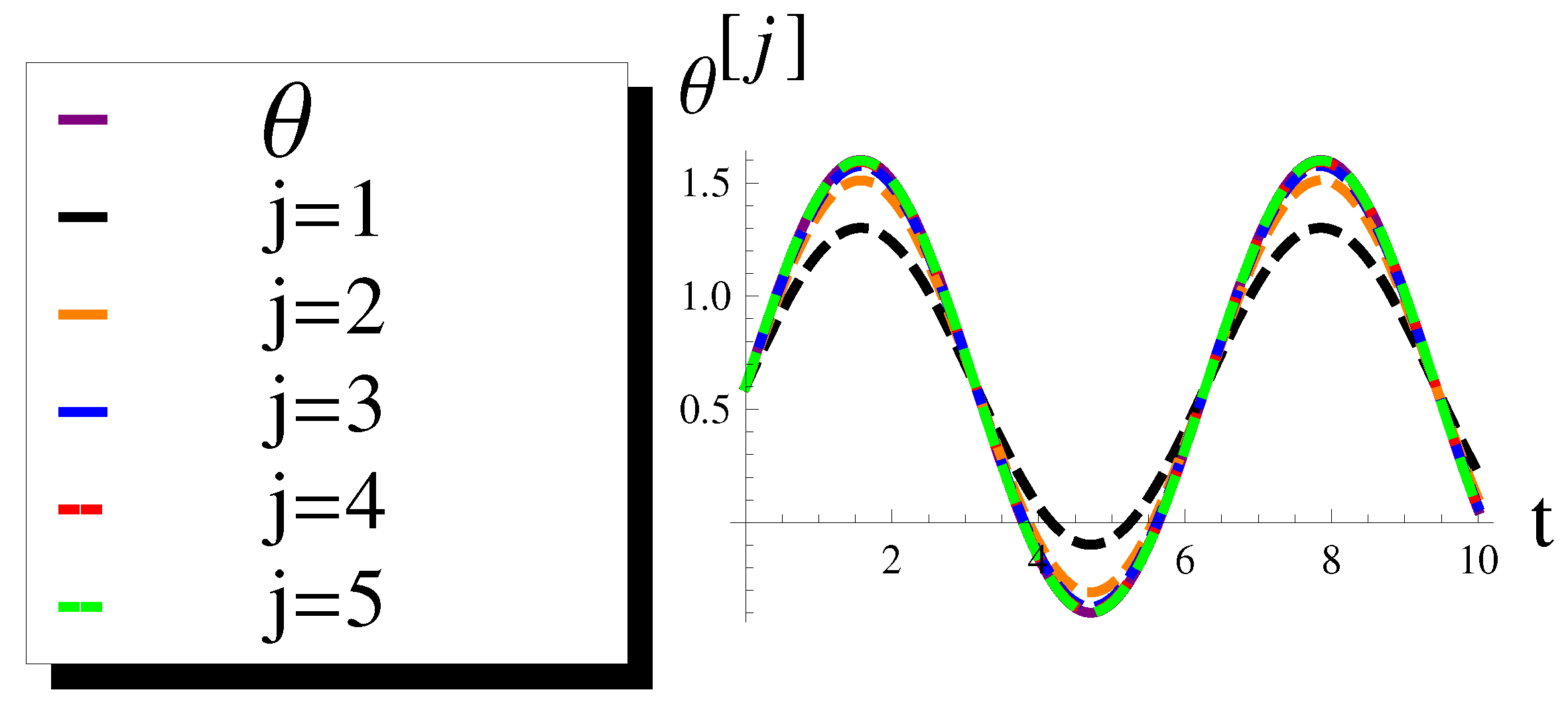
Figure 8 shows the plots of the truncated series solution using different number of terms together with the corresponding analytical exact solution of Example 4 at x = 0.7 and = 0.7 . It shows that the truncated series solution of order j = 5 is very close to the exact solution, which indicates the rapid convergence of the proposed method.
Table 4 presents the absolute error E r [ j ] = | θ ( x , t ) θ [ j ] ( x , t ) | due to the difference between the exact solution and the approximate solution of various orders of Example 4 at different values of x and t. It illustrates the rapid convergence of the approximate solution obtained by using this method.

5. Conclusions

In this article, a numerical scheme is developed to solve a mathematical model subject to a non-local condition of integral type by combining two well known methods; the double Laplace transform and the homotopy analysis method. The derived scheme is applied on a set of test examples to demonstrate it’s reliability and efficiency. This scheme generates the exact solution for each one of these example. The convergence of the obtained approximate solutions is tested graphically as shown in Figure 2, Figure 4, Figure 6, and Figure 8. These figures show rapid convergence of the numerical solutions towards the exact solution just after few iterations. The error in these approximate solutions is computed for several values of the independent variables x and t, and it is presented in Table 1, Table 2, Table 3 and Table 4. These tables reflect the efficiency and accuracy of the proposed method using few terms of the truncated series solutions. These results show that the HADLTM is an efficient technique for solving this problem, and any other similar problems.

Author Contributions

Conceptualization, S.M.; methodology, S.M. and H.E.G.; software, S.M. and I.B.; validation, S.M. and I.B.; formal analysis, S.M. and H.E.G.; resources, S.M. and H.E.G.; investigation, S.M. and I.B. All authors have read and agreed to the published version of the manuscript.

Funding

Researchers Supporting Project number (RSPD2023R975) King Saud University, Riyadh, Saudi Arabia.

Data Availability Statement

Not applicable.

Acknowledgments

The author extend his appreciation to the Researchers Supporting Project Number (RSPD2023R975) King Saud University, Riyadh Saudi Arabia.

Conflicts of Interest

The author declare no conflict of interest in this paper.

References

  1. Muravei, L.A.; Philinovskii, A.V. On a certain nonlocal boundary value problem for hyperbolic equation. Matem. Zametki 1993, 54, 98–116. [Google Scholar]
  2. Nakhushev, A.N. An approximate method for solving boundary value problems for differential equations and its application to the dynamics of ground moisture and ground water. Differ. Uravn. 1982, 18, 72–81. [Google Scholar]
  3. Pulkina, L.S. A nonlocal problem with integral conditions for hyperbolic equations. Electron. J. Differ. Equ. 1999, 45, 1–6. [Google Scholar] [CrossRef]
  4. Pulkina, L.S. On the solvability in L2 of a nonlocal problem with integral conditions for a hyperbolic equation. Differ. Equ. 2000, 36, 316–318. [Google Scholar] [CrossRef]
  5. Samarskii, A.A. Some problems in differential equations theory. Differ. Uravn. 1980, 16, 1221–1228. [Google Scholar]
  6. Shi, P.; Shillor, M. Design of Contact Patterns in One Dimensional Thermoelasticity in Theoretical Aspects of Industrial Design; Society for Industrial and Applied Mathematics: Philadelphia, PA, USA, 1992. [Google Scholar]
  7. Cannon, J.R. The solution of heat equation subject to the specification of energy. Q. Appl. Math. 1963, 21, 155–160. [Google Scholar] [CrossRef]
  8. Ionkin, N.I.; Moiseev, E.I. A problem for heat conduction equation with two point boundary condition. Differ. Uravn. 1979, 15, 1284–1295. [Google Scholar]
  9. Kacur, J.; van Keer, R. On the numerical solution of semilinear parabolic problems in multicomponent structures with Volterra operators in the transmission conditions and in the boundary conditions. Z. Fuer Angew. Math. Und Mech. 1995, 75, 91–103. [Google Scholar] [CrossRef]
  10. Dehghan, M. The one-dimensional heat equation subject to a boundary integral specification. Chaos Solitons Fractals 2007, 32, 661–675. [Google Scholar] [CrossRef]
  11. Taki-Eddine, O.; Abdelfatah, B.; Gattal, N. Numerical Solution of Mixed Problem of Parabolic Equation with an Integral Conditions by using Finite Difference and Orthogonal Function Approximation. Math. Moravica 2012, 16, 89–98. [Google Scholar] [CrossRef]
  12. Ramezani, M.; Dehghan, M.; Razzaghi, M. Combined finite difference and spectral methods for the numerical solution of hyperbolic equation with an integral condition. Numer. Methods Partial. Differ. Equ. 2008, 24, 1–8. [Google Scholar] [CrossRef]
  13. Singh, H. Chebyshev spectral method for solving a class of local and nonlocal elliptic boundary value problems. Int. J. Nonlinear Sci. Numer. Simul. 2023, 24, 899–915. [Google Scholar] [CrossRef]
  14. Gudi, T. Finite element method for a nonlocal problem of Kirchhoff type. SIAM J. Numer. Anal. 2012, 50, 657–668. [Google Scholar] [CrossRef]
  15. Chang, S.H.; Chang, I.L. A new algorithm for calculating one-dimensional differential transform of nonlinear functions. Appl. Math. Comput. 2008, 195, 799–808. [Google Scholar] [CrossRef]
  16. Arikoglu, A.; Ozkol, I. Solution of fractional differential equations by using differential transform method. Chaos Solitons Fractals 2007, 34, 1473–1481. [Google Scholar] [CrossRef]
  17. Adomian, G. Nonlinear Stochastic Operator Equations; Kluwer Academic Publishers: Alphen aan den Rijn, The Netherlands, 1986; ISBN 978-0-12-044375-8. [Google Scholar]
  18. Adomian, G. A Review of the Decomposition Method in Applied Mathematics. J. Math. Anal. Appl. 1988, 135, 501–544. [Google Scholar] [CrossRef]
  19. Adomian, G. A review of the decomposition method and some recent results for nonlinear equations. Comput. Math. Appl. 1991, 21, 101–127. [Google Scholar]
  20. Khuri, S.A. A Laplace decomposition algorithm applied to a class of nonlinear differential equations. J. Appl. Math. 2001, 1, 141–155. [Google Scholar] [CrossRef]
  21. Khuri, S.A. A new approach to Bratu’s problem. Appl. Math. Comput. 2004, 147, 131–136. [Google Scholar] [CrossRef]
  22. He, J.H. Variational iteration method a kind of non-linear analytical technique: Some examples. Int. J. Non-Linear Mech. 1999, 34, 699–708. [Google Scholar] [CrossRef]
  23. He, J.H. Variational iteration method for autonomous ordinary differential systems. Appl. Math. Comput. 2000, 114, 115–123. [Google Scholar] [CrossRef]
  24. He, J.H. Homotopy perturbation technique. Comput. Methods Appl. Mech. Eng. 1999, 178, 257–262. [Google Scholar] [CrossRef]
  25. He, J.H. A coupling method of a homotopy technique and a perturbation technique for non-linear problems. Int. J. Nonlinear Mech. 2000, 35, 37–43. [Google Scholar] [CrossRef]
  26. He, J.H. New interpretation of homotopy perturbation method. Int. J. Mod. Phys. B 2006, 20, 2561–2568. [Google Scholar] [CrossRef]
  27. Liao, S.J. The Proposed Homotopy Analysis Technique for the Solution of Nonlinear Problems. Ph.D. Thesis, Shanghai Jiao Tong University, Shanghai, China, 1992. [Google Scholar]
  28. Liao, S.J. Homotopy analysis method a new analytical technique for nonlinear problems. Commun. Nonlinear Sci. Numer. Simul. 1997, 2, 95–100. [Google Scholar] [CrossRef]
  29. Liao, S.J. An explicit, totally analytic approximation of Blasius’ viscous flow problems. Int. J. Non-Linear Mech. 1999, 34, 759–778. [Google Scholar] [CrossRef]
  30. Liao, S.J. Beyond Perturbation: Introduction to the Homotopy Analysis Method; Chapman & Hall/CRC Press: Boca Raton, FL, USA, 2003; ISBN 978-1-58488-407-1. [Google Scholar]
  31. Liao, S.J. On the homotopy analysis method for nonlinear problems. Appl. Math. Comput. 2004, 147, 499–513. [Google Scholar] [CrossRef]
  32. Mesloub, S.; Obaidat, S. On the application of the homotopy analysis method for a nonlocal mixed problem with Bessel operator. Appl. Math. Comput. 2012, 219, 3477–3485. [Google Scholar] [CrossRef]
  33. Eltayeb, H.; Kiliçman, A. A note on solutions of wave, Laplace’s and heat equations with convolution terms by using a double Laplace transform. Appl. Math. Lett. 2008, 21, 1324–1329. [Google Scholar] [CrossRef]
  34. Kiliçman, A.; Eltayeb, H. A note on defining singular integral as distribution and partial differential equations with convolution term. Math. Comput. Model. 2009, 49, 327–336. [Google Scholar] [CrossRef]
  35. Kiliçman, A.; Gadain, H.E. On the applications of Laplace and Sumudu transforms. J. Frankl. Inst. 2010, 347, 848–862. [Google Scholar] [CrossRef]
  36. Mesloub, S.; Bouziani, A. Mixed problem with a weighted integral condition for a parabolic equation with the Bessel operator. J. Appl. Math. Stoch. Anal. 2000, 15, 277–286. [Google Scholar] [CrossRef]
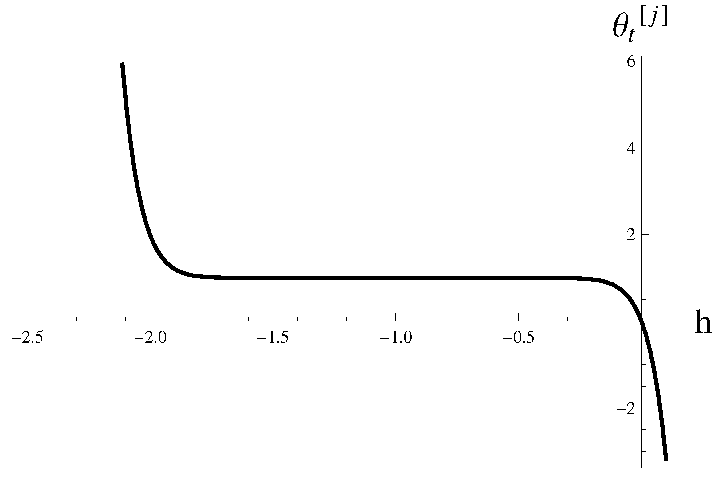
Figure 1. The -curve corresponding to the 15th order series solution at t = 0 .
Axioms 12 00933 g001
Figure 2. Approximate solution θ [ j ] ( x , t ) with various values of j together with the exact solution θ ( x , t ) of Example 1.
Axioms 12 00933 g002
Figure 3. The -curve corresponding to the 16th order approximate solution at t = 0 .
Axioms 12 00933 g003
Figure 4. Approximate solution θ [ j ] ( x , t ) with various values of j together with the exact solution θ ( x , t ) of Example 2.
Axioms 12 00933 g004
Figure 5. The -curve corresponding to the 15th order series solution at t = 0 .
Axioms 12 00933 g005
Figure 6. Approximate solution θ [ j ] ( x , t ) with various values of j together with the exact solution θ ( x , t ) of Example 3.
Axioms 12 00933 g006
Figure 7. The -curve for the 15th order series solution at t = 0 .
Axioms 12 00933 g007
Figure 8. Approximate solution θ [ j ] ( x , t ) with various values of j together with the exact solution θ ( x , t ) of Example 3.
Axioms 12 00933 g008
Table 1. Absolute error at = 0.9 and different values of j, x, and t.
t
0.10.515
x j Er [ j ] Er [ j ] Er [ j ] Er [ j ]
0.120.0010.0050.010.05
51 × 10 6 5 × 10 6 0.000010.00005
101 × 10 11 5.00002 × 10 11 1.00001 × 10 10 5.00003 × 10 10
14 1.33227 × 10 15 5.55112 × 10 15 1.15463 × 10 14 5.59552 × 10 14
0.520.0010.0050.010.05
51 × 10 6 5 × 10 6 0.000010.00005
10 1.00001 × 10 11 5.00004 × 10 11 1.00001 × 10 10 5.00003 × 10 10
14 1.22125 × 10 15 5.66214 × 10 15 1.13243 × 10 14 5.59552 × 10 14
0.720.0010.0050.010.05
51 × 10 6 5 × 10 6 0.000010.00005
10 1.00001 × 10 11 5.00003 × 10 11 1.00001 × 10 10 5.00002 × 10 10
14 1.11022 × 10 15 5.55112 × 10 15 1.13243 × 10 14 5.50671 × 10 14
0.920.0010.0050.010.05
51 × 10 6 5 × 10 6 0.000010.00005
10 1.00001 × 10 11 5.00004 × 10 11 1.00001 × 10 10 5.00002 × 10 10
14 1.11022 × 10 15 5.66214 × 10 15 1.13243 × 10 14 5.50671 × 10 14
Table 2. Absolute error at = 0.9 and different values of j, x, and t.
t
0.10.515
x j Er [ j ] Er [ j ] Er [ j ] Er [ j ]
0.120.00010.00250.010.25
51 × 10 7 2.5 × 10 6 0.000010.00025
10 1.00009 × 10 12 2.50004 × 10 11 1.00001 × 10 10 2.50003 × 10 9
14 8.88178 × 10 16 2.4869 × 10 14 9.9698 × 10 14 2.51887 × 10 12
0.520.00010.00250.010.25
51 × 10 7 2.5 × 10 6 0.000010.00025
10 9.99978 × 10 13 2.50002 × 10 11 1.00001 × 10 10 2.50003 × 10 9
14 1.11022 × 10 16 2.83107 × 10 15 1.12133 × 10 14 2.4869 × 10 13
0.720.00010.00250.010.25
51 × 10 7 2.5 × 10 6 0.000010.00025
10 9.99978 × 10 13 2.50002 × 10 11 1.00001 × 10 10 2.50003 × 10 9
14 1.11022 × 10 16 2.77556 × 10 15 1.12133 × 10 14 2.4869 × 10 13
0.920.00010.00250.010.25
51 × 10 7 2.5 × 10 6 0.000010.00025
10 9.99978 × 10 13 2.50002 × 10 11 1.00001 × 10 10 2.50003 × 10 9
14 1.11022 × 10 16 2.77556 × 10 15 1.11022 × 10 14 2.4869 × 10 13
Table 3. Absolute error at = 1.1 and different values of j, x, and t.
t
0.10.515
x j Er [ j ] Er [ j ] Er [ j ] Er [ j ]
0.120.001812690.006321210.008646650.00999955
5 1.81269 × 10 6 6.32121 × 10 6 8.64665 × 10 6 9.99955 × 10 6
10 1.81267 × 10 11 6.32119 × 10 11 8.64666 × 10 11 9.99953 × 10 11
14 1.77636 × 10 15 6.43929 × 10 15 8.88178 × 10 15 1.02141 × 10 14
0.520.001812690.006321210.008646650.00999955
5 1.81269 × 10 6 6.32121 × 10 6 8.64665 × 10 6 9.99955 × 10 6
10 1.81268 × 10 11 6.32121 × 10 11 8.64664 × 10 11 9.99955 × 10 11
14 1.77636 × 10 15 6.32827 × 10 15 8.71525 × 10 15 1.00475 × 10 14
0.720.001812690.006321210.008646650.00999955
5 1.81269 × 10 6 6.32121 × 10 6 8.64665 × 10 6 9.99955 × 10 6
10 1.81268 × 10 11 6.32121 × 10 11 8.64665 × 10 11 9.99955 × 10 11
14 1.77636 × 10 15 6.32827 × 10 15 8.6875 × 10 15 1.00475 × 10 14
0.920.001812690.006321210.008646650.00999955
5 1.81269 × 10 6 6.32121 × 10 6 8.64665 × 10 6 9.99955 × 10 6
10 1.81268 × 10 11 6.32121 × 10 11 8.64665 × 10 11 9.99955 × 10 11
14 1.77636 × 10 15 6.30052 × 10 15 8.65974 × 10 15 1.00475 × 10 14
Table 4. Absolute error at = 1.1 and different values of j, x, and t.
t
0.10.515
x j Er [ j ] Er [ j ] Er [ j ] Er [ j ]
0.120.0009983340.004794260.008414710.00958924
5 9.98334 × 10 7 4.79426 × 10 6 8.41471 × 10 6 9.58924 × 10 6
10 9.98357 × 10 12 4.79425 × 10 11 8.41469 × 10 11 9.58926 × 10 11
14 8.88178 × 10 16 4.88498 × 10 15 7.99361 × 10 15 9.76996 × 10 15
0.520.0009983340.004794260.008414710.00958924
5 9.98334 × 10 7 4.79426 × 10 6 8.41471 × 10 6 9.58924 × 10 6
10 9.98324 × 10 12 4.79425 × 10 11 8.41469 × 10 11 9.58925 × 10 11
14 8.88178 × 10 16 4.88498 × 10 15 7.99361 × 10 15 9.63118 × 10 15
0.720.0009983340.004794260.008414710.00958924
5 9.98334 × 10 7 4.79426 × 10 6 8.41471 × 10 6 9.58924 × 10 6
10 9.98324 × 10 12 4.79425 × 10 11 8.41469 × 10 11 9.58925 × 10 11
14 8.88178 × 10 16 4.88498 × 10 15 7.99361 × 10 15 9.65894 × 10 15
0.920.0009983340.004794260.008414710.00958924
5 9.98334 × 10 7 4.79426 × 10 6 8.41471 × 10 6 9.58924 × 10 6
10 9.98335 × 10 12 4.79425 × 10 11 8.41469 × 10 11 9.58925 × 10 11
14 9.99201 × 10 16 4.77396 × 10 15 8.21565 × 10 15 9.65894 × 10 15
Disclaimer/Publisher’s Note: The statements, opinions and data contained in all publications are solely those of the individual author(s) and contributor(s) and not of MDPI and/or the editor(s). MDPI and/or the editor(s) disclaim responsibility for any injury to people or property resulting from any ideas, methods, instructions or products referred to in the content.