Adaptive Type-II Hybrid Progressive Censoring Samples for Statistical Inference of Comparative Inverse Weibull Distributions

Abstract

Recently, there has been a lot of interest in comparative life testing for items under jointly censored schemes for products from multiple production lines. The inverse Weibull distribution (IWD) is commonly used in life testing and reliability theory. In this paper, we address the problem of statistical inference from comparative inverse Weibull distributions under joint samples. An adaptive type-II hybrid progressive censoring scheme (HPCS) is used to save the balance between the ideal test time and the number of observed failures. Under the adaptive type-II HPCS, unknown parameters of the inverse Weibull populations are estimated using both maximum likelihood and Bayesian approaches. Asymptotic confidence intervals are established using the observed Fisher information matrix and bootstrap confidence intervals. We suggest using Markov chain Monte Carlo (MCMC) techniques to compute credible intervals under independent gamma priors. Using Monte Carlo simulations, all theoretical conclusions are tested and contrasted. For illustration purposes, an actual sample from comparative populations is analysed.

1. Introduction

The inverse Weibull distribution (IWD) is employed as a lifetime model in the reliability engineering discipline. The density and hazard function of the IWD might be unimodal or declining, depending on the form of the parameter used. As a result, if empirical studies confirm that the hazard function is unimodal, the IWD fits the data better than the Weibull distribution. The following examples highlight the significance of the IWD: the IWD is more useful for modelling several failure characteristics, including wear-out periods, infant mortality, and the time to breakdown of an insulating fluid subjected to the effect of constant strain. Furthermore, the IWD is a viable model for describing the failure of mechanical components in diesel engines. In situations where units consist of several parts and the failure of each part has the same distribution, Weibull and inverse Weibull distributions are more acceptable for modelling; see Liu [1] and Nelson [2]. A comparison between Weibull and inverse Weibull composite distributions was performed by Cooray and colleagues [3]. The parameters of IWD were estimated under adaptive type-II progressive hybrid censoring scheme, see Nassar and Abo-Kasem [4]. For entropy estimation of the IWD, see Xu and Gui [5], and for modelling reliability data, see Alkarni et al. [6]. The random variable T has an inverse Weibull random variable if the probability density function (PDF) is

$$f\left(t\right)=\alpha \beta t^{-\left(\beta +1\right)}{e}^{-\alpha t^{-\beta }},\alpha ,\beta >0,t>0,$$

(1)

where $\alpha$ and $\beta$ are the scale and shape parameters, respectively. Figure 1 was plotted using Mathematica version 10 to show the different shapes of PDFs and the corresponding hazard failure rate (HFR) function of the IWD for the scale parameter $\alpha =1.0$ and different parameters $\beta .$

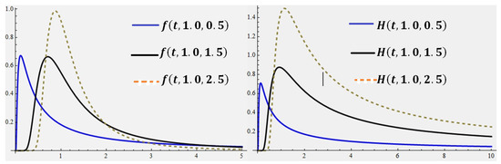
Figure 1. The PDF and the corresponding hazard failure rate function of the IWD.

To determine the reliability of any product, certain product units must be submitted to a life testing trial, and the resulting lifetime data may be complete or censored. The cost and duration of the test determine the best approach for collecting data. In the literature, common and simple censoring schemes are known as type-I and type-II censoring schemes (CSs). If a random sample of size n is randomly selected from a life population, under the type-I CS, the test time is proposed but the number of failures r is random, $0\le r\le n$. In contrast, in the type-II CS, the test time is random but the number of failures is proposed beforehand. It is that the number of failures r is randomly selected in the type-I CS; the test has a lack of memory and r may be zero. However, in the type-II CS, the test time $T_m$ is random and it may be that $T_m\to \infty$. This is more conventional in several cases. The ideal test time $\tau$ and the number of failures m are proposed beforehand in the hybrid censoring scheme (HCS). Therefore, when the type-I CS is combined with the HCS design, type-I HCS is presented. In the type-I HCS and the type-II HCS, the experimenter terminates the experiment at min($\tau ,$ $T_m$) and max($\tau ,$ $T_m$), respectively. The last two types of censoring schemes type-I HCS and type-II HCS have the same lack of memory (i.e., a small number of failures and a higher test time, respectively). Type-I and type-II CSs or type-I and type-II HCSs do not allow for the removal of units from the test other than the final point. The concept of removing units other than the final point is allowed in progressive censoring schemes (PCSs) and hybrid progressive censoring schemes (HPCSs), see Balakrishnan and Aggarwala [7] and Balakrishnan [8].

For type-II PCSs, a random sample of units of size n is tested. The number of failures m and the CS $\mathbf{R}=(R_1,$ $R_2,$ $\dots ,$ $R_m)$ are proposed beforehand. When the experiment is running at each failure time $T_{i:m,n},$ $i=$ 1, 2, …, m, $R_i$ survival units are randomly removed from the test. The experiment is continued until the failure time $T_{m:m,n}$ is reached and then the remaining $R_m$ survival units are removed from the test. Then, the random sample $\mathbf{T}=(T_{1;m,n}^{\mathbf{R}},$ $T_{2;m,n}^{\mathbf{R}},$ $\dots ,$ $T_{m;m,n}^{\mathbf{R}})$ is called the type-II PC sample. In contrast, for the type-I HPCS, a sample of size n is put under testing. The number of failures m, the ideal test time $\tau$, and the CS $\mathbf{R}=(R_1,$ $R_2,$ $\dots ,$ $R_m)$ are proposed beforehand. As given in type-II PCSs, at each failure time $T_{i:m,n},$ $i=$1, 2, …, r and $r\le m,R_i$ survival units are randomly removed from the test. The experiment is continued until the time $\tau$ is reached and the remaining $n-r-{\displaystyle \sum _{i=r}^m}{r}_i$ survival units are removed from the test. The random sample $\mathbf{T}=(T_{1;m,n}^{\mathbf{R}},$ $T_{2;m,n}^{\mathbf{R}},$ $\dots ,$ $T_{r;m,n}^{\mathbf{R}})$ is called a type-I HPC sample. Censoring type-I HPC and type-II PC schemes both lack memory, resulting in a small number of failures and a larger test time, respectively. In practice, a problem arises from choosing suitable censorship schemes, which balance the effective number of failures needed for statistical inference and a short test time. Ng et al. [9] proposed a new model called adaptive type-II HPCS, which saves both the cost and the time; see Abd-Elmougod et al. [10] for further information about adaptive type-II HPCS. The experiment design under adaptive type-II HPCS introduced statistical inference efficiency, where a threshold time can be employed to switch from the originally planned censoring scheme to a changed one. Comparative lifetime studies are particularly important in manufacturing processes for determining the relative qualities of many competing products in terms of reliability. The joint censoring scheme (JCS) has recently received a lot of attention, and it is especially significant in comparing the lives of units from various manufacturing lines. Many studies have considered the problem of JCS, such as Bhattacharyya and Mehrotra [11], and Mehrotra and Bhattacharyya [12]. Also, further discussion of JCS is presented by Balakrishnan and Rasouli [13], Rasouli and Balakrishnan [14], and Shafay et al. [15]. The balanced JCS under PCS is given by Mondal and Kundu [16] and recently discussed by Algarni et al. [17] and Tahani et al. [18]. For other recent works on JCS, one can refer to Almarashi et al. [19], Shokr et al. [20], Tolba et al. [21], and Al-Essa et al. [22]. One of the more important subjects in the statistical literature is the statistical inference of comparative life populations. This issue is investigated since the life item has IWD and all of the parameters are unknown. As a result, the purpose of this study is to provide statistical inference for comparing IW lifetime populations. We employed this problem under adaptive type-II HPCS with a joint censoring scheme to create the joint adaptive type-II HPCS. To create point and interval estimators for comparative population parameters, maximum likelihood (ML) and Bayesian estimating methodologies are used. Asymptomatic properties of the ML estimations are used to calculate asymptotic confidence intervals. Bootstrap confidence intervals are also provided. In the Bayesian technique, the parameters are assumed to have independent gamma priors. Bayes estimates, as expected, cannot be obtained in closed form. In this case, we use the Metropolis–Hastings MH with Gibbs sampling technique to generate samples from the posterior distributions and then compute the Bayes estimators of the individual parameters, and Bayesian credible intervals are then calculated. The performance of classical and Bayes estimators is compared using several simulated trials. The rest of the paper is summarised as follows: Section 2 describes the model with the joint adaptive type-II hybrid censoring scheme as well as some assumptions. In Section 3, we obtain the traditional maximum likelihood estimators and asymptotic confidence intervals. Bayes point estimation with a credible interval are proposed in the same Section. Section 4, illustrates the analysis of a real-life data set that represents failure times of breakdown of an insulated fluid. Also, the numerical assessment of the developed results from the simulation study are provided in Section 4. The brief comments with our conclusion and recommendations are reported in Section 5.

2. Joint Adaptive Type-II Hybrid Censoring Scheme

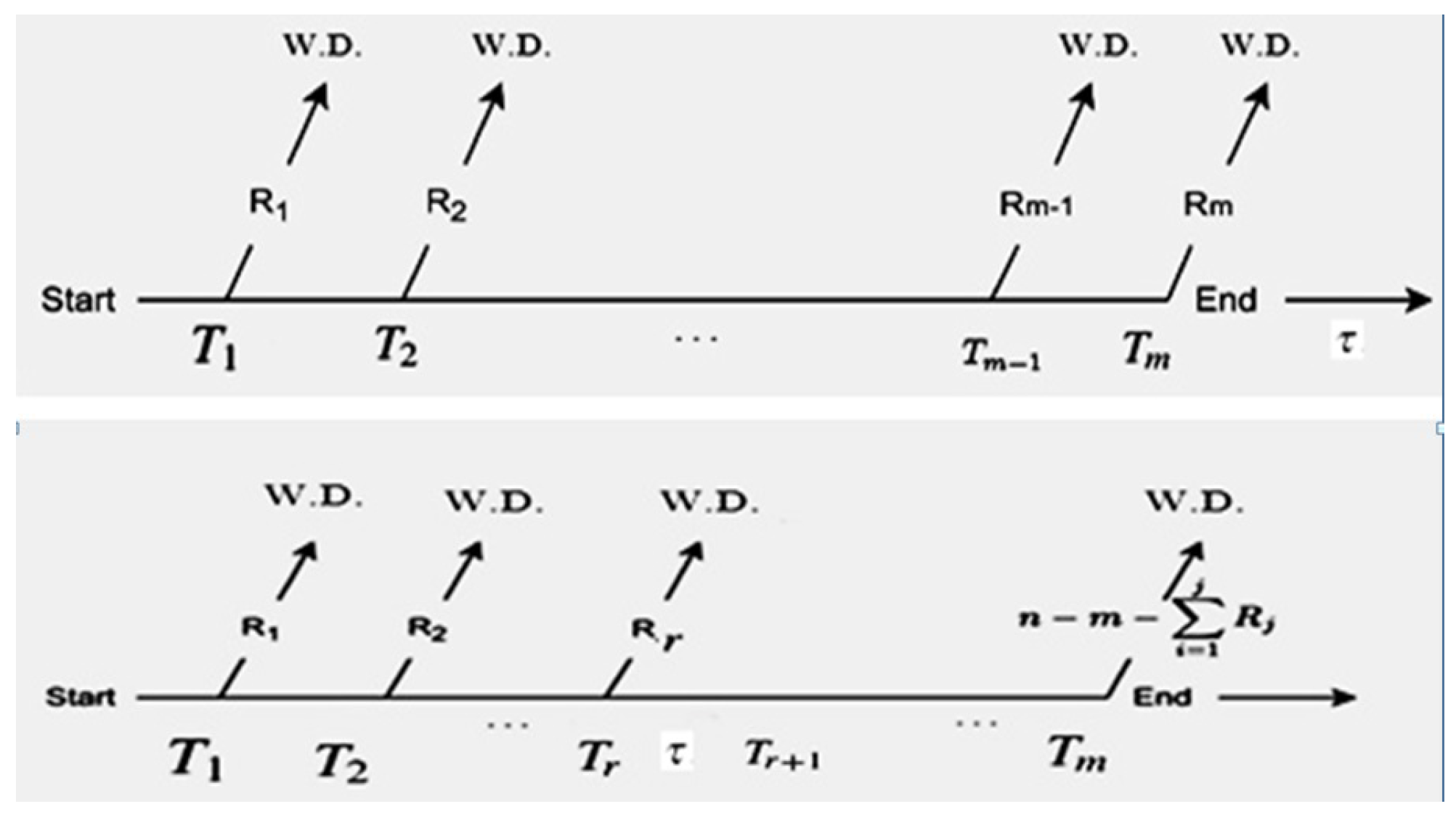
A joint random sample of size n is selected from a two comparative life product to put under a life-testing experiment. Suppose that a random sample of size n is taken from two lines of production, such that $n_1$ from line ${\Phi }_1$ and $n_2$ from line ${\Phi }_2,$ $n=n_1+n_2.$ The mechanism of joint adaptive type-II HPCS can be described as follows: let the pairs ($m,$ $\tau$) denote the number of observed failures and the ideal test time, with the censoring scheme $\mathbf{R}=(R_1,$ $R_2,$ $\dots ,$ $R_m)$ being proposed. When the experiment is running, the failure time and the corresponding type ($T_i,{\eta }_i$) are recorded. On observing the first failure $T_1$ and the corresponding type ${\eta }_1,$ we record ($T_1,{\eta }_1$) and $R_1$ survival units are randomly removed from the test. When the second failure $T_2$ is observed, then we record ($T_2,{\eta }_2$) and $R_2$ survival units are removed from the test. The experiment is continued until the time $\tau$ is reached, $T_r<\tau <$ $T_{r+1},$ $1\le r<m$ and $T_0=0$, $T_{m+1}=\infty .$ If m-th failures are observed before the time $\tau$, then the experiment is terminated at time $T_m$. But if $T_m>\tau$ (which means that the number of failures r is smaller than $m)$, then we need to terminate the experiment as soon as possible. Then, the observed joint adaptive type-II HPCS is given as: $\mathbf{T}=${($T_1$, ${\eta }_1$), ($T_2$, ${\eta }_2$)$,\dots ,$ ($T_r$, ${\eta }_r$), ($T_{r+1}$, ${\eta }_{r+1}$), …, $(T_m$, ${\eta }_m\left)\right\}.$ For more details, see David and Nagaraja [23] and Ng and Chan [24]. Therefore, under adaptive type-II HPCS, the scheme $\mathbf{R}=(R_1,$ $R_2,$ $\dots ,$ $R_m)$ change to ${\mathbf{R}}^{*}=(R_1,$ $R_2,$ $\dots ,$ $R_r,$ $0,$ $0,$ $\dots ,$ $0,$ $R_m^{*}),$ $R_m^{*}=n-m-{\displaystyle \sum _{i=1}^r}{R}_i$. The time $\tau$ is essential for the modification $\mathbf{R}$ to ${\mathbf{R}}^{*}$ (reduced the total test time). It should be noted that, when $\tau =0,$ the adaptive type-II HPCS is reduced to ordinary type-II CS, and when $\tau \to \infty$, it is reduced to ordinary type-II PCS. Figure 2 was drawn to present the different cases of adaptive type-II HPCS.

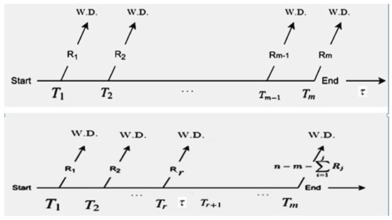
Figure 2. Adaptive type-II HPCS when $T_m<\tau$, (top) and $T_m>\tau$, (bottom).

Let $m_1={\displaystyle \sum _{i=1}^m}{\eta }_i$ and $m_2={\displaystyle \sum _{i=1}^m}(1-{\eta }_i)$ are number of observed failure from lines ${\Phi }_1$ and ${\Phi }_2,$ respectively (where ${\eta }_i=1$ mean from the line ${\Phi }_1$ and ${\eta }_i=0$ mean from the line ${\Phi }_2).$

Under consideration that two lines ${\Phi }_1$ and ${\Phi }_2$ of production with units have PDFs, and CDFs follow the IWD lifetime distribution defined by:

$$f_j\left(t\right)={\alpha }_j{\beta }_j{t}^{-\left({\beta }_j+1\right)}{e}^{-{\alpha }_j{t}^{-{\beta }_j}},{\alpha }_j,{\beta }_j>0,t>0,j=1,2,$$

(2)

with the corresponding CDFs, reliability, and failure rate functions

$$F_j\left(t\right)=e^{-{\alpha }_j{t}^{-{\beta }_j}},$$

(3)

$$S_j\left(t\right)=1-e^{-{\alpha }_j{t}^{-{\beta }_j}},$$

(4)

and

$$H_j\left(t\right)=\frac{{\alpha }_j{\beta }_j{t}^{-\left({\beta }_j+1\right)}{e}^{-{\alpha }_j{t}^{-{\beta }_j}}}{1-e^{-{\alpha }_j{t}^{-{\beta }_j}}}.$$

(5)

Suppose that the failure times $X_1,$ $X_2,$ $\dots ,X_{n_1}$ are observed from the line ${\Phi }_1$, which have a cumulative distribution function (CDF) and probability density function (PDF), given respectively, by $F_1(.)$ and $f_1(.).$ Also, let the failure times $Y_1,$ $Y_2,$ $\dots ,Y_{n_2}$ belong to the line ${\Phi }_2$ with CDF and PDF, given respectively, by $F_2(.)$ and $f_2(.).$ For a given data of size m and test time $\tau ,$ the ordered life times {$T_1,$ $T_2,$ $\dots ,$ $T_r,$ $T_{r+1},\dots ,T_m\},$ obtained from the joint sample $\{X_1,X_2,\dots ,X_{m_1},$ $Y_1,$ $Y_2,$ $\dots ,Y_{m_2}\}$ with $m=m_1+m_2$ is called a joint adaptive type-II HPC sample.

The likelihood function of the observed joint adaptive type-II HPC sample $\mathbf{T}=${($T_1$, ${\eta }_1$), ($T_2$, ${\eta }_2$)$,\dots ,$ ($T_r$, ${\eta }_r$), ($T_{r+1}$, ${\eta }_{r+1}$), …, $(T_m$, ${\eta }_m\left)\right\}$ is formulated by:  

$$f(t_1,t_2,\dots ,t_r,t_{r+1},\dots ,t_m|\Theta )=A{\displaystyle \prod _{i=1}^m}{\left[f_1\left(t_i\right)\right]}^{{\eta }_i}{\left[f_2\left(t_i\right)\right]}^{1-{\eta }_i}{\left[S_1\left(t_i\right)\right]}^{R_{1i}^{*}}{\left[S_2\left(t_i\right)\right]}^{R_{2i}^{*}},$$

(6)

where $R_{1i}^{*}+R_{2i}^{*}=R_i^{*}$ denote the number of survival units removed from the lines ${\Phi }_1$ and ${\Phi }_2.$ Also, $\Theta$ is the parameters vectors, $S_j(.)=1-F_j(.),$ $j=1,$ $2,$ with

$$0<t_1<t_2<\dots <t_r<t_{r+1}<\dots <t_m<\infty ,$$

$$A={\displaystyle \prod _{i=1}^m}\left[n-i+1-{\displaystyle \sum _{i=1}^{min\left\{i-1,J\right\}}}{R}_i\right],$$

(7)

and

$$R_i^{\ast }=\left\{\begin{array}{cc}{R}_i& \mathrm{if}i\le r\\ 0& \mathrm{if}r<i<m\\ \hfill {}^{n-m-{\displaystyle \sum _{j=1}^r}Rj}& \mathrm{if}i=m\mathrm{and}r<m.\end{array}\right.$$

(8)

3. Methodology

3.1. Point Estimation

In this section, we formulate the point estimations of the model parameters and some parameters of life (reliability and hazard failure rate functions) by using classical and Bayesian approaches.

3.1.1. ML Estimation

For the given joint sample $\mathbf{T}=${($T_1$, ${\eta }_1$), ($T_2$, ${\eta }_2$)$,\dots ,$ ($T_r$, ${\eta }_r$), ($T_{r+1}$, ${\eta }_{r+1}$), …, $(T_m$, ${\eta }_m\left)\right\}$ and IWD distribution given by (2)–(4), the joint likelihood function is

$$\begin{array}{cc}\hfill L\left(\Theta |\mathbf{T}\right)& \propto {\alpha }_1^{m_1}{\alpha }_2^{m_2}{\beta }_1^{m_1}{\beta }_2^{m_2}{\displaystyle \prod _{i=1}^m}{\left[t_i^{-\left({\beta }_1+1\right)}{e}^{-{\alpha }_1{t}_i^{-{\beta }_1}}\right]}^{{\eta }_i}{(1-e^{-{\alpha }_1{t}_i^{-{\beta }_1}})}^{R_{1i}^{\ast }}{\left[t_i^{-\left({\beta }_2+1\right)}{e}^{-{\alpha }_2{t}_i^{-{\beta }_2}}\right]}^{1-{\eta }_i}\hfill \\ \hfill & \times {(1-e^{-{\alpha }_2{t}_i^{-{\beta }_2}})}^{R_{2i}^{\ast }},\hfill \end{array}$$

(9)

where $\Theta =\{{\alpha }_1,$ ${\alpha }_2,$ ${\beta }_1,$ ${\beta }_2\}.$ The natural logarithm of the likelihood function is given by

$$\begin{array}{cc}\hfill \ell \left(\Theta |\mathbf{T}\right)& =m_{1}log{\alpha }_1+m_{2}log{\alpha }_2+m_{1}log{\beta }_1+m_{2}log{\beta }_2-\left({\beta }_1+1\right){\displaystyle \sum _{i=1}^m}{\eta }_{i}log{t}_i-{\alpha }_1{\displaystyle \sum _{i=1}^m}{\eta }_i{t}_i^{-{\beta }_1}\hfill \\ \hfill & +{\displaystyle \sum _{i=1}^m}{R}_{1i}^{\ast }log\left[1-e^{-{\alpha }_1{t}_i^{-{\beta }_1}}\right]-\left({\beta }_2+1\right){\displaystyle \sum _{i=1}^m}(1-{\eta }_i)log{t}_i-{\alpha }_2{\displaystyle \sum _{i=1}^m}(1-{\eta }_i)t_i^{-{\beta }_2}\hfill \\ \hfill & +{\displaystyle \sum _{i=1}^m}{R}_{2i}^{\ast }log\left[1-e^{-{\alpha }_2{t}_i^{-{\beta }_2}}\right],\hfill \end{array}$$

(10)

by taking the first partial derivatives of (10) with respect to the model parameters $\Theta =\{{\alpha }_1,$ ${\alpha }_2,$ ${\beta }_1,$ ${\beta }_2\},$ and equating them zero, the following likelihood equations are obtained:

$$\frac{\partial \ell \left(\Theta |\mathbf{T}\right)}{\partial {\alpha }_1}=\frac{m_1}{{\alpha }_1}-{\displaystyle \sum _{i=1}^m}{\eta }_i{t}_i^{-{\beta }_1}+{\displaystyle \sum _{i=1}^m}{R}_{1i}^{\ast }\frac{t_i^{-{\beta }_1}{e}^{-{\alpha }_1{t}_i^{-{\beta }_1}}}{1-e^{-{\alpha }_1{t}_i^{-{\beta }_1}}}=0,$$

(11)

$$\frac{\partial \ell \left(\Theta |\mathbf{T}\right)}{\partial {\alpha }_2}=\frac{m_2}{{\alpha }_2}-{\displaystyle \sum _{i=1}^m}(1-{\eta }_i)t_i^{-{\beta }_2}+{\displaystyle \sum _{i=1}^m}{R}_{2i}^{\ast }\frac{t_i^{-{\beta }_2}{e}^{-{\alpha }_2{t}_i^{-{\beta }_2}}}{1-e^{-{\alpha }_2{t}_i^{-{\beta }_2}}}=0,$$

(12)

$$\begin{array}{cc}\hfill & \frac{\partial \ell \left(\Theta |\mathbf{T}\right)}{\partial {\beta }_1}=\frac{m_1}{{\beta }_1}-{\displaystyle \sum _{i=1}^m}{\eta }_{i}log{t}_i+{\alpha }_1{\displaystyle \sum _{i=1}^m}{\eta }_i{t}_i^{-{\beta }_1}log{t}_i-{\alpha }_1{\displaystyle \sum _{i=1}^m}{R}_i^{\ast }\frac{t_i^{-{\beta }_1}log{t}_i{e}^{-{\alpha }_1{t}_i^{-{\beta }_1}}}{1-e^{-{\alpha }_1{t}_i^{-{\beta }_1}}}=0,\hfill \end{array}$$

(13)

and

$$\begin{array}{cc}\hfill & \frac{\partial \ell \left(\Theta |\mathbf{T}\right)}{\partial {\beta }_2}=\frac{m_2}{{\beta }_2}-{\displaystyle \sum _{i=1}^m}(1-{\eta }_i)log{t}_i+{\alpha }_2{\displaystyle \sum _{i=1}^m}(1-{\eta }_i)t_i^{-{\beta }_2}log{t}_i-{\alpha }_2{\displaystyle \sum _{i=1}^m}{R}_{2i}^{\ast }\frac{t_i^{-{\beta }_2}log{t}_i{e}^{-{\alpha }_2{t}_i^{-{\beta }_2}}}{1-e^{-{\alpha }_2{t}_i^{-{\beta }_2}}}=0.\hfill \end{array}$$

(14)

The nonlinear Equations (11)–(14) do not admit explicit solutions. Therefore, the Newton–Raphson iteration methods are used to solve them and to obtain the ML estimates $\widehat{\Theta }=\{{\widehat{\alpha }}_1,$ ${\widehat{\alpha }}_2,$ ${\widehat{\beta }}_1,$ ${\widehat{\beta }}_2\}.$ It should be noted that the numerical manipulations in this paper were carried out using the Mathematica package (Mathematica ver. 10). In Mathematica, the FindRoot module uses Newton’s method to solve a nonlinear system. Also, the FindRoot module uses a damped version of Newton–Raphson, for without the damping, bad choices of starting values will more often result in divergence. The damping makes the iterations less likely to go wild. As a consequence of the invariance property of the ML estimator, we can obtain the ML estimators of the reliability and hazard failure rate functions as

$${\widehat{S}}_j\left(t\right)=1-e^{-{\widehat{\alpha }}_j{t}^{-{\widehat{\beta }}_j}},$$

(15)

and

$${\widehat{H}}_j\left(t\right)=\frac{{\widehat{\alpha }}_j{\widehat{\beta }}_j{t}^{-\left({\widehat{\beta }}_j+1\right)}{e}^{-{\widehat{\alpha }}_j{t}^{-{\widehat{\beta }}_j}}}{1-e^{-{\widehat{\alpha }}_j{t}^{-{\widehat{\beta }}_j}}}.$$

(16)

3.1.2. Bayesian Estimation

The Bayesian approach is dependent on the prior information of the model parameters and information in the data presented by the likelihood function. The problem of choosing suitable prior information is more important in the statistical literature. The gamma distribution has a maximum entropy probability distribution, and the main motivation for the gamma prior is usually to constrain the random variables to positive values. Also, the gamma distribution is considered a family of distributions, and each of the exponential and chi-square distributions is considered a special case. Therefore, in this study, independent gamma priors are assumed for all parameters, as follows:

$${\Pi }_i^{*}\left({\Theta }_i\right)\propto {\Theta }_i^{a_i-1}exp(-b_i{\Theta }_i),{\Theta }_i>0;a_i,b_i>0,i=1,\dots ,4,$$

(17)

where $\Theta =\{{\alpha }_1,$ ${\alpha }_2,$ ${\beta }_1,$ ${\beta }_2\}.$ The corresponding joint density function of prior distribution is given by

$${\Pi }^{\ast }({\alpha }_1,{\alpha }_2,{\beta }_1,{\beta }_2)\propto {\alpha }_1^{a_1-1}{\alpha }_2^{a_2-1}{\beta }_1^{a_3-1}{\beta }_2^{a_4-1}exp(-b_1{\alpha }_1-b_2{\alpha }_2-b_3{\beta }_1-b_4{\beta }_2).$$

(18)

The joint posterior density function is formulated from (9) and (18) by

$$\begin{array}{cc}\hfill & \Pi ({\alpha }_1,{\alpha }_2,{\beta }_1,{\beta }_2|\mathbf{T})\propto {\alpha }_1^{m_1+a_1-1}{\alpha }_2^{m_2+a_2-1}{\beta }_1^{m_1+a_3-1}{\beta }_2^{m_2+a_4-1}exp\left\{-\left({\beta }_1+1\right){\displaystyle \sum _{i=1}^m}{\eta }_{i}log{t}_i\right.\hfill \\ \hfill & -b_1{\alpha }_1-b_3{\beta }_1-{\alpha }_1{\displaystyle \sum _{i=1}^m}{\eta }_i{t}_i^{-{\beta }_1}+{\displaystyle \sum _{i=1}^m}{R}_{1i}^{\ast }log\left[1-e^{-{\alpha }_1{t}_i^{-{\beta }_1}}\right]-\left({\beta }_2+1\right){\displaystyle \sum _{i=1}^m}(1-{\eta }_i)log{t}_i\hfill \\ \hfill & \left.-b_2{\alpha }_2-b_4{\beta }_2-{\alpha }_2{\displaystyle \sum _{i=1}^m}(1-{\eta }_i)t_i^{-{\beta }_2}+{\displaystyle \sum _{i=1}^m}{R}_{2i}^{\ast }log\left[1-e^{-{\alpha }_2{t}_i^{-{\beta }_2}}\right]\right\}.\hfill \end{array}$$

(19)

The joint posterior distribution (19) has shown that, under a high-dimensional case, the posterior distribution and the corresponding Bayes estimators cannot be simplified to a closed form. Therefore, different methods can be applied to obtain the Bayes estimators of the model parameters, such as Lindely approximation, numerical integration and the Markov Chen Monte Carlo (MCMC) method. In the following subsection, we discuss the MCMC method.

3.1.3. MCMC Method

The full conditional posterior distributions obtained from (19) are formulated by:

$${\Pi }_1\left({\alpha }_1\right|{\alpha }_2,{\beta }_1,{\beta }_2,\mathbf{T})\propto {\alpha }_1^{m_1+a_1-1}exp\left\{-{\alpha }_1\left(b_1+{\displaystyle \sum _{i=1}^m}{\eta }_i{t}_i^{-{\beta }_1}\right)\right\},$$

(20)

$${\Pi }_2\left({\alpha }_2\right|{\alpha }_1,{\beta }_1,{\beta }_2,\mathbf{T})\propto {\alpha }_2^{m_2+a_2-1}exp\left\{-{\alpha }_2\left(b_2+{\displaystyle \sum _{i=1}^m}(1-{\eta }_i)t_i^{-{\beta }_2}\right)\right\},$$

(21)

$${\Pi }_3\left({\beta }_1\right|{\alpha }_1,{\alpha }_2,{\beta }_2,\mathbf{T})\propto {\beta }_1^{m_1+a_3-1}exp\left\{-{\beta }_1\left(b_3+{\displaystyle \sum _{i=1}^m}{\eta }_{i}log{t}_i\right)\right\},$$

(22)

and

$${\Pi }_4\left({\beta }_1\right|{\alpha }_1,{\alpha }_2,{\beta }_2,\mathbf{T})\propto {\beta }_2^{m_2+a_4-1}exp\left\{-{\beta }_2\left(b_4+{\displaystyle \sum _{i=1}^m}(1-{\eta }_i)log{t}_i\right)\right\},$$

(23)

with the associated weight

$$h({\alpha }_1,{\alpha }_2,{\beta }_1,{\beta }_2|\mathbf{T})=\frac{exp\left\{{\displaystyle \sum _{i=1}^m}{R}_{1i}^{*}log\left[1-e^{-{\alpha }_1{t}_i^{-{\beta }_1}}\right]+{\displaystyle \sum _{i=1}^m}{R}_{2i}^{*}log\left[1-e^{-{\alpha }_2{t}_i^{-{\beta }_2}}\right]\right\}}{{\left(b_1+{\displaystyle \sum _{i=1}^m}{\eta }_i{t}_i^{-{\beta }_1}\right)}^{m_1+a_1}{\left(b_2+{\displaystyle \sum _{i=1}^m}(1-{\eta }_i)t_i^{-{\beta }_2}\right)}^{m_2+a_2}}.$$

(24)

   The empirical posterior distribution is obtained with the help of the subclass of the MCMC method for the full conditional distributions (20) to (23). Moreover, since the functions in (20)–(23) follow gamma, it is quite simple to generate from these functions. So, we provide the importance sampling procedure to compute the Bayes estimates according to the following Algorithm 1:

Algorithm 1: Importance sample algorithm

1. Put $\kappa =1$ and begin with initial guess value of ${\Theta }^{\left(0\right)}=\{{\widehat{\alpha }}_1,$ ${\widehat{\alpha }}_2,$ ${\widehat{\beta }}_1,$ ${\widehat{\beta }}_2\}$. 2. The values ${\alpha }_j^{\left(\kappa \right)},$ $j=1,$ $2,$ is generated from gamma distributions given by (20) and (21). 3. The values ${\beta }_j^{\left(\kappa \right)},$ $j=1,$ $2,$ is generated from gamma distributions given by (22) and (23). 4. Compute $h({\alpha }_1^{\left(\kappa \right)},{\alpha }_2^{\left(\kappa \right)},{\beta }_1^{\left(\kappa \right)},{\beta }_2^{\left(\kappa \right)}|\mathbf{T})$ 5. Put $\kappa$ = $\kappa +1.$ 6. Steps from (2) to (5) is repeated $\mathbf{MC}$ times. 7. Under consideration that, ${\mathbf{MC}}^{*}$ is the number of MCMC iteration need to reaching the stationary distribution. The Bayes estimate of any function $\Psi ({\alpha }_1,{\alpha }_2,{\beta }_1,{\beta }_2)$ of the model parameters under squared error loss function is given by $${\widehat{\Psi }}_{\mathrm{B}}={\mathrm{E}}_{\Pi }(\Psi |\mathbf{T})=\frac{\frac{1}{\mathbf{MC}-{\mathbf{MC}}^{*}}{\displaystyle \sum _{j={\mathbf{MC}}^{*}+1}^{\mathbf{MC}}}\Psi ({\alpha }_1^{\left(j\right)},{\alpha }_2^{\left(j\right)},{\beta }_1^{\left(j\right)},{\beta }_2^{\left(j\right)})h({\alpha }_1^{\left(j\right)},{\alpha }_2^{\left(j\right)},{\beta }_1^{\left(j\right)},{\beta }_2^{\left(j\right)}|\mathbf{T})}{\frac{1}{\mathbf{MC}-{\mathbf{MC}}^{*}}{\displaystyle \sum _{j={\mathbf{MC}}^{*}+1}^{\mathbf{MC}}}h({\alpha }_1^{\left(j\right)},{\alpha }_2^{\left(j\right)},{\beta }_1^{\left(j\right)},{\beta }_2^{\left(j\right)}|\mathbf{T})},$$ (25) and the corresponding posterior variance is $$\widehat{V}(\Psi )=\frac{\frac{1}{\mathbf{MC}-{\mathbf{MC}}^{*}}{\displaystyle \sum _{j={\mathbf{MC}}^{*}+1}^{\mathbf{MC}}}{({\Psi }^{\left(j\right)}-{\widehat{\Psi }}_{\mathrm{B}})}^{2}h({\alpha }_1^{\left(j\right)},{\alpha }_2^{\left(j\right)},{\beta }_1^{\left(j\right)},{\beta }_2^{\left(j\right)}|\mathbf{T})}{\frac{1}{\mathbf{MC}-{\mathbf{MC}}^{*}}{\displaystyle \sum _{j={\mathbf{MC}}^{*}+1}^{\mathbf{MC}}}h({\alpha }_1^{\left(j\right)},{\alpha }_2^{\left(j\right)},{\beta }_1^{\left(j\right)},{\beta }_2^{\left(j\right)}|\mathbf{T})},$$ (26)

3.2. Interval Estimation

In this section, we discussed the interval estimation of the model parameters. Firstly, we discuss classical estimation (asymptotic ML confidence intervals and bootstrap confidence intervals). Secondly, we present Bayesian credible intervals.

3.2.1. Asymptotic Confidence Intervals

The Fisher information matrix (FIM) is used to formulate interval estimators of the model parameters. FIM is defined as the expectation of a minus second derivative of the log-likelihood function. In the cases in which this expectation is more serious, we replace FIM with approximate information matrix (AIM), which is defined by

$$\mathrm{AIM}(\Theta )=-\left(\frac{{\partial }^2\ell \left(\Theta |\mathbf{T}\right)}{\partial {\Theta }_i\partial {\Theta }_k}\right){|}_{i,k=1,2,3,4}.$$

(27)

    Under the property that the ML estimators of the model parameters $\Theta =\{{\alpha }_1,$ ${\alpha }_2,$ ${\beta }_1,$ ${\beta }_2\}$ have a bivariate normal distribution with mean $\Theta =\{{\alpha }_1,$ ${\alpha }_2,$ ${\beta }_1,$ ${\beta }_2\}$ and a variance covariance matrix obtained from the inverse of the AIM at the ML estimate defined by

$${\mathrm{AIM}}^0=-\left(\frac{{\partial }^2\ell \left(\Theta |\mathbf{T}\right)}{\partial {\Theta }_i\partial {\Theta }_k}\right){|}_{{\widehat{\alpha }}_1,{\widehat{\alpha }}_2,{\widehat{\beta }}_1,{\widehat{\beta }}_2}.$$

(28)

The approximate ($1-\gamma$)%100 confidence intervals of $\Theta =\{{\alpha }_1,$ ${\alpha }_2,$ ${\beta }_1,$ ${\beta }_2\}$ is given

$$\left\{\begin{array}{c}{\widehat{\alpha }}_j\mp {\omega }_{\frac{\gamma }{2}}{z}_j,j=1,2,\\ {\widehat{\beta }}_j\mp {\omega }_{\frac{\gamma }{2}}{z}_{j+2j+2},j=1,2,\end{array}\right.,$$

(29)

where the the elements of the diagonal of AIM⁰ take the values $z_j,$ $j=$1, …, 4. And the value ${\omega }_{\frac{\gamma }{2}}$ is a standard normal value under significant level $\gamma .$

3.2.2. Bootstrap Confidence Intervals

Using the bootstrap technique, we can compute any quantity of interest by re-sampling from the pseudo-population. In this subsection, we use the bootstrap method to re-sample and then produce the confidence interval, which can be applied to statistical inference with a small effective sample size. We adopted the percentile parametric bootstrap technique to formulate the confidence interval of the model parameters. For information about bootstrap-p, see Efron [25]. Algorithm 2, can be used to compute parametric bootstrap-p confidence intervals.

3.2.3. Bayesian HP Credible Interval

Bayesian HP credible intervals of the model parameters $\Theta =\{{\alpha }_1,$ ${\alpha }_2,$ ${\beta }_1,$ ${\beta }_2\}$ are obtained by using the idea of Chen and Shao [26]. The algorithms used to formulate HP credible intervals of the model parameters can be described as follows.

Step 1 

From the MCMC sample ${\Theta }^{\left(i\right)}=\{{\alpha }_1^{\left(i\right)},$ ${\alpha }_2^{\left(i\right)},$ ${\beta }_1^{\left(i\right)},$ ${\beta }_2^{\left(i\right)}\}$, $i={\mathbf{MC}}^{*}+1,$ ${\mathbf{MC}}^{*}+2,$ …, $\mathbf{MC}$ generated by the importance sampling technique.

Step 2 

Sort ${\Theta }_k^{\left(i\right)},k=1,2,3,4$ to obtain the ordered values, ${\Theta }_{k\left(i\right)}.$

Step 3 

Compute the weighted function $w_i$

$$w_i=\frac{h({\alpha }_1^{\left(i\right)},{\alpha }_2^{\left(i\right)},{\beta }_1^{\left(i\right)},{\beta }_2^{\left(i\right)}|\mathbf{T})}{{\displaystyle \sum _{j={\mathbf{MC}}^{*}+1}^{\mathbf{MC}}}h({\alpha }_1^{\left(i\right)},{\alpha }_2^{\left(i\right)},{\beta }_1^{\left(i\right)},{\beta }_2^{\left(i\right)}|\mathbf{T})}.$$

(30)

Then, rewrite $(w_i,i={\mathbf{MC}}^{*}+1,$ ${\mathbf{MC}}^{*}+2,$ $\dots ,$ $\mathbf{MC})$ as $(w_{\left(i\right)},i=1,$ $2,$ $\dots ,$ $\mathbf{MC}-{\mathbf{MC}}^{*})$ so that the i-th value $w_{\left(i\right)}$ corresponds to the the value ${\Theta }_{k\left(i\right)}$.

Step 4 

The $\gamma -$quantile of the marginal posterior of ${\Theta }_{k\left(i\right)}$ can be estimated by

$${\tilde{\Theta }}_k{}^{\left(\gamma \right)}=\left\{\begin{array}{c}{\Theta }_{k\left(1\right)},\mathrm{if}\gamma =0\hfill \\ \multicolumn{1}{c}{{\Theta }_{k\left(j\right)},\mathrm{if}{\displaystyle \sum _{i=1}^{j-1}}{w}_{\left(i\right)}<\gamma <{\displaystyle \sum _{i=1}^j}{w}_{\left(i\right)}}\end{array}.\right.$$

(31)

Step 5 

Compute the $(1-\gamma )100\%$ credible intervals of $\theta$

$$[{\theta }^{\frac{L}{\mathbf{MC}-{\mathbf{MC}}^{*}}},{\theta }^{(\frac{L+(1-\gamma )(\mathbf{MC}-{\mathbf{MC}}^{*})}{\mathbf{MC}-{\mathbf{MC}}^{*}})}],$$

(32)

where $L=1,2,\dots ,\gamma (\mathbf{MC}-{\mathbf{MC}}^{*}).$

Step 6 

The ($1-\gamma$)100% HPD interval is the one with the smallest interval width among all credible intervals.

Algorithm 2: Bootstrap-p confidence intervals

From the original data set $\mathbf{T}=$ {($T_1$, ${\eta }_1$), ($T_2$, ${\eta }_2$)$,\dots ,$ ($T_r$, ${\eta }_r$), ($T_{r+1}$, ${\eta }_{r+1}$), …, $(T_m$, ${\eta }_m\left)\right\},$ compute $\widehat{\Theta }=\{{\widehat{\alpha }}_1,$ ${\widehat{\alpha }}_2,$ ${\widehat{\beta }}_1,$ ${\widehat{\beta }}_2\}$. Generate two samples of sizes $n_1$ and $n_2$ from IWD(${\widehat{\alpha }}_1,$ ${\widehat{\beta }}_1$) and IWD(${\widehat{\alpha }}_2,$ ${\widehat{\beta }}_2$), respectively. From the joint sample of size $n_1$ + $n_2,$ generate random type-II PC sample of size m by using the algorithms given by Balakrishnan and Sandhu [27]. Form the random type-II PC sample of size m for given $\tau ,$ report the sample {$T_1,$ $T_2,$ $\dots ,$ $T_r\}$, $r\le m.$ Generate two samples of size ($m-r$) from truncated distributions, see Ng et al. [9] and choose the smallest ($m-r$) values from the joint sample. Report the bootstrap joint adaptive type-II HPC sample and its type ${\mathbf{T}}^{\ast }=${$T_1^{\ast },$ $T_2^{\ast },$ $\dots ,$ $T_r^{\ast },$ $T_{r+1}^{\ast },\dots ,T_m^{\ast }\}.$ Based on ${\mathbf{T}}^{\ast }=${$T_1^{\ast },$ $T_2^{\ast },$ $\dots ,$ $T_r^{\ast },$ $T_{r+1}^{\ast },\dots ,T_m^{\ast }\}$, compute ${\Theta }^{\ast \left(0\right)}=\{{\widehat{\alpha }}_1^{\ast },$ ${\widehat{\alpha }}_2^{\ast },$ ${\widehat{\beta }}_1^{\ast },$ ${\widehat{\beta }}_2^{\ast }\}.$ Repeat the Steps (2–6) MB times, we have ${\widehat{\Theta }}^{\ast \left(i\right)}=\{{\widehat{\alpha }}_1^{\ast \left(i\right)},$ ${\widehat{\alpha }}_2^{\ast \left(i\right)},$ ${\widehat{\beta }}_1^{\ast \left(i\right)},$ ${\widehat{\beta }}_2^{\ast \left(i\right)}\},$ $i=$1, 2, …, MB. Put, the bootstrap sample estimate in ascending order as ${\widehat{\Theta }}_{\left(i\right)}^{\ast }=\{{\widehat{\alpha }}_{1\left(i\right)}^{\ast },$ ${\widehat{\alpha }}_{2\left(i\right)}^{\ast },$ ${\widehat{\beta }}_{1\left(i\right)}^{\ast },$ ${\widehat{\beta }}_{2\left(i\right)}^{\ast }\},$ $i=$1, 2, …, MB. The cumulative distribution function of ${\widehat{\Theta }}_{\left(i\right)}^{\ast }$ can be defined by $\mathsf{ϝ}\left({\widehat{\Theta }}_k^{\ast }\right)=P({\widehat{\Theta }}_k^{\ast }⩽z),$ ${\widehat{\Theta }}_1^{\ast }={\widehat{\alpha }}_1^{\ast }$ and others. Hence, $(1-\gamma )100\%$ percentile Bootstrap confidence intervals is given by $$\left[{\widehat{\Theta }}_{k\mathrm{boot}}^{\ast }\left(\frac{\gamma }{2}\right),{\widehat{\Theta }}_{k\mathrm{boot}}^{\ast }(1-\frac{\gamma }{2})\right].$$

4. Numerical Results

4.1. Simulation Studies

To determine the quality of the ML and Bayesian estimation methods discussed in the preceding sections, a Monte Carlo simulation study is conducted. Some measures are computed, such as the mean squared error for the point estimation and the mean interval length and coverage percentage for the interval estimation. In this study, we consider different sample sizes, different effective sample sizes, and different choices for censoring schemes, with varying values of the ideal test time. The parameters $\{{\alpha }_1,{\alpha }_2,{\beta }_1,{\beta }_2\}$ are chosen to be (2.0, 1.0, 0.5, 0.8) and (1.0, 0.5, 1.5, 2.0). For the Bayesian estimation, we have taken both informative (P${}^1$) and non-informative priors (P${}^0$), and the hyperparameter values are chosen so that the expectation of the prior distributions is equivalent to the true value. In the simulation study, we generate 1000 samples with the pre-specified model parameters. For each sample, we compute the point ML and Bayes estimates and the mean estimate (ME) with the corresponding mean squared error (MSE). For interval estimations, we compute average interval length (AIL) and coverage percentage (CP). We adopted four censoring schemes (CS) defined as:

scheme I: $R_m=n_1+n_2-m,R_i=0$ for $i\ne m.$

scheme II: $R_i=0,$ $i=1,2,\dots ,n_1+n_2-m$, $R_i=1,$ $i=n_1+n_2-m,\dots ,n_1+n_2.$

scheme III: $R_i=1$ for $i=1,$ $2,$ $\dots ,$ m, $R_i=0$ for $i=m+1,$ $2,$ $\dots ,$ $n_1+n_2$.

scheme IV: $R_1=n_1+n_2-m,$ $R_i=0$ for $i\ne 1.$

The results of the simulation study are computed according to Algorithm 3:   

Algorithm 3: Monte Carlo simulation study

For given $\Theta =\{{\alpha }_1,{\alpha }_2,{\beta }_1,{\beta }_2\}$, generate two samples of sizes $n_1$ and $n_2$ from IWD(${\alpha }_1$, ${\beta }_1$) and IWD(${\alpha }_2$, ${\beta }_2$), respectively. From the joint sample of size $n_1$+$n_2$, randomly generate type-II PC sample of size m. Under comparison between the ideal test time $\tau ,$ with type-II PC sample of size m report the sample {$T_1,$ $T_2,$ $\dots ,$ $T_r\}$, $r\le m.$ Generate two samples of size ($m-r$) from truncated IWDs see Ng et al. [9] and choose the smallest ($m-r$) values. Report the joint adaptive type-II HPC sample $\mathbf{T}=${($T_1$, ${\eta }_1$), ($T_2$, ${\eta }_2$)$,\dots ,$ ($T_r$, ${\eta }_r$), ($T_{r+1}$, ${\eta }_{r+1}$), …, $(T_m$, ${\eta }_m\left)\right\}$. Steps from 1 to 4 are repeated 1000 times. For each adaptive type-II HPC sample we compute the MLE and Bayes estimates (point and interval). The mean estimate ME and MSE are computed and reported in Table 1 and Table 2. The results of point estimates show ML and non-informative Bayes estimates are close to each other. Therefore, the AIL and CP are computed and reported in Table 3 and Table 4 for informative Bayes credible intervals.

Table 1. ME and MSE of the parameter estimates for $\Theta =$ {2.0, 1.0, 0.5, 0.8}.

				MLE				Bayes(P${}^0$)				Bayes(P${}^1$)
$\mathit{\tau }$	(${\mathit{n}}_{\mathbf{1}}\mathbf{,}{\mathit{n}}_{\mathbf{2}}\mathbf{,}\mathit{m}$)	CS		${\mathit{\alpha }}_{\mathbf{1}}$	${\mathit{\beta }}_{\mathbf{1}}$	${\mathit{\alpha }}_{\mathbf{2}}$	${\mathit{\beta }}_{\mathbf{2}}$	${\mathit{\alpha }}_{\mathbf{1}}$	${\mathit{\beta }}_{\mathbf{1}}$	${\mathit{\alpha }}_{\mathbf{2}}$	${\mathit{\beta }}_{\mathbf{2}}$	${\mathit{\alpha }}_{\mathbf{1}}$	${\mathit{\beta }}_{\mathbf{1}}$	${\mathit{\alpha }}_{\mathbf{2}}$	${\mathit{\beta }}_{\mathbf{2}}$
0.5	(20,20,15)	I	ME	2.345	0.734	1.298	1.098	2.311	0.701	1.254	1.071	2.281	0.667	1.178	1.001
			MSE	0.321	0.147	0.224	0.200	0.301	0.132	0.207	0.193	0.301	0.132	0.207	0.193
		II	ME	2.338	0.739	1.277	1.077	2.288	0.698	1.251	1.062	2.254	0.648	1.170	0.978
			MSE	0.307	0.132	0.207	0.183	0.281	0.112	0.200	0.179	0.286	0.114	0.191	0.177
		III	ME	2.318	0.722	1.265	1.070	2.269	0.682	1.239	1.049	2.241	0.633	1.159	0.966
			MSE	0.288	0.111	0.188	0.166	0.264	0.092	0.181	0.161	0.265	0.100	0.177	0.168
		IV	ME	2.310	0.708	1.249	1.058	2.255	0.671	1.230	1.037	2.232	0.620	1.148	0.954
			MSE	0.255	0.092	0.171	0.152	0.248	0.081	0.168	0.145	0.249	0.081	0.160	0.152
	(30,30,35)	I	ME	2.241	0.645	1.200	0974	2.228	0.633	1.192	0966	2.187	0.556	1.099	0901
			MSE	0.204	0.069	0.124	0.099	0.189	0.063	0.112	0.093	0.102	0.044	0.089	0.045
		II	ME	2.237	0.640	1.192	0968	2.221	0.625	1.188	0958	2.180	0.548	1.092	0893
			MSE	0.189	0.061	0.117	0.087	0.166	0.052	0.101	0.079	0.088	0.032	0.078	0.033
		III	ME	2.231	0.634	1.187	0961	2.214	0.614	1.180	0947	2.171	0.539	1.085	0885
			MSE	0.180	0.053	0.108	0.081	0.154	0.048	0.089	0.072	0.082	0.028	0.071	0.029
		IV	ME	2.224	0.629	1.182	0954	2.200	0.602	1.171	0942	2.165	0.533	1.080	0877
			MSE	0.165	0.044	0.098	0.073	0.145	0.040	0.075	0.064	0.077	0.018	0.064	0.023
1.0	(20,20,15)	I	ME	2.338	0.728	1.291	1.093	2.302	0.687	1.248	1.070	2.271	0.658	1.172	1.003
			MSE	0.312	0.138	0.215	0.192	0.294	0.123	0.199	0.187	0.293	0.125	0.201	0.189
		II	ME	2.332	0.740	1.278	1.071	2.279	0.691	1.244	1.058	2.255	0.639	1.162	0.971
			MSE	0.301	0.128	0.202	0.174	0.273	0.104	0.193	0.171	0.278	0.107	0.180	0.169
		III	ME	2.309	0.724	1.258	1.066	2.269	0.677	1.233	1.043	2.238	0.627	1.154	0.961
			MSE	0.281	0.103	0.179	0.161	0.258	0.088	0.174	0.157	0.261	0.097	0.166	0.161
		IV	ME	2.312	0.711	1.241	1.047	2.251	0.667	1.227	1.031	2.224	0.613	1.141	0.950
			MSE	0.247	0.090	0.166	0.143	0.241	0.074	0.162	0.138	0.242	0.074	0.152	0.145
	(30,30,35)	I	ME	2.233	0.640	1.201	0969	2.223	0.628	1.187	0961	2.182	0.548	1.092	0897
			MSE	0.193	0.062	0.119	0.092	0.181	0.054	0.103	0.087	0.093	0.041	0.082	0.041
		II	ME	2.229	0.632	1.188	0961	2.217	0.614	1.182	0949	2.171	0.540	1.087	0888
			MSE	0.183	0.054	0.112	0.088	0.167	0.055	0.093	0.073	0.082	0.027	0.073	0.028
		III	ME	2.224	0.631	1.182	0958	2.211	0.609	1.178	0943	2.173	0.532	1.081	0881
			MSE	0.174	0.049	0.102	0.076	0.142	0.03	0.084	0.066	0.074	0.022	0.065	0.023
		IV	ME	2.218	0.622	1.175	0947	2.192	0.595	1.173	0935	2.161	0.524	1.082	0871
			MSE	0.161	0.039	0.092	0.066	0.140	0.032	0.071	0.055	0.072	0.014	0.059	0.018

Table 1. ME and MSE of the parameter estimates for $\Theta =$ {2.0, 1.0, 0.5, 0.8}.

				MLE				Bayes(P${}^0$)				Bayes(P${}^1$)
$\mathit{\tau }$	(${\mathit{n}}_{\mathbf{1}}\mathbf{,}{\mathit{n}}_{\mathbf{2}}\mathbf{,}\mathit{m}$)	CS		${\mathit{\alpha }}_{\mathbf{1}}$	${\mathit{\beta }}_{\mathbf{1}}$	${\mathit{\alpha }}_{\mathbf{2}}$	${\mathit{\beta }}_{\mathbf{2}}$	${\mathit{\alpha }}_{\mathbf{1}}$	${\mathit{\beta }}_{\mathbf{1}}$	${\mathit{\alpha }}_{\mathbf{2}}$	${\mathit{\beta }}_{\mathbf{2}}$	${\mathit{\alpha }}_{\mathbf{1}}$	${\mathit{\beta }}_{\mathbf{1}}$	${\mathit{\alpha }}_{\mathbf{2}}$	${\mathit{\beta }}_{\mathbf{2}}$
0.5	(20,20,15)	I	ME	2.345	0.734	1.298	1.098	2.311	0.701	1.254	1.071	2.281	0.667	1.178	1.001
			MSE	0.321	0.147	0.224	0.200	0.301	0.132	0.207	0.193	0.301	0.132	0.207	0.193
		II	ME	2.338	0.739	1.277	1.077	2.288	0.698	1.251	1.062	2.254	0.648	1.170	0.978
			MSE	0.307	0.132	0.207	0.183	0.281	0.112	0.200	0.179	0.286	0.114	0.191	0.177
		III	ME	2.318	0.722	1.265	1.070	2.269	0.682	1.239	1.049	2.241	0.633	1.159	0.966
			MSE	0.288	0.111	0.188	0.166	0.264	0.092	0.181	0.161	0.265	0.100	0.177	0.168
		IV	ME	2.310	0.708	1.249	1.058	2.255	0.671	1.230	1.037	2.232	0.620	1.148	0.954
			MSE	0.255	0.092	0.171	0.152	0.248	0.081	0.168	0.145	0.249	0.081	0.160	0.152
	(30,30,35)	I	ME	2.241	0.645	1.200	0974	2.228	0.633	1.192	0966	2.187	0.556	1.099	0901
			MSE	0.204	0.069	0.124	0.099	0.189	0.063	0.112	0.093	0.102	0.044	0.089	0.045
		II	ME	2.237	0.640	1.192	0968	2.221	0.625	1.188	0958	2.180	0.548	1.092	0893
			MSE	0.189	0.061	0.117	0.087	0.166	0.052	0.101	0.079	0.088	0.032	0.078	0.033
		III	ME	2.231	0.634	1.187	0961	2.214	0.614	1.180	0947	2.171	0.539	1.085	0885
			MSE	0.180	0.053	0.108	0.081	0.154	0.048	0.089	0.072	0.082	0.028	0.071	0.029
		IV	ME	2.224	0.629	1.182	0954	2.200	0.602	1.171	0942	2.165	0.533	1.080	0877
			MSE	0.165	0.044	0.098	0.073	0.145	0.040	0.075	0.064	0.077	0.018	0.064	0.023
1.0	(20,20,15)	I	ME	2.338	0.728	1.291	1.093	2.302	0.687	1.248	1.070	2.271	0.658	1.172	1.003
			MSE	0.312	0.138	0.215	0.192	0.294	0.123	0.199	0.187	0.293	0.125	0.201	0.189
		II	ME	2.332	0.740	1.278	1.071	2.279	0.691	1.244	1.058	2.255	0.639	1.162	0.971
			MSE	0.301	0.128	0.202	0.174	0.273	0.104	0.193	0.171	0.278	0.107	0.180	0.169
		III	ME	2.309	0.724	1.258	1.066	2.269	0.677	1.233	1.043	2.238	0.627	1.154	0.961
			MSE	0.281	0.103	0.179	0.161	0.258	0.088	0.174	0.157	0.261	0.097	0.166	0.161
		IV	ME	2.312	0.711	1.241	1.047	2.251	0.667	1.227	1.031	2.224	0.613	1.141	0.950
			MSE	0.247	0.090	0.166	0.143	0.241	0.074	0.162	0.138	0.242	0.074	0.152	0.145
	(30,30,35)	I	ME	2.233	0.640	1.201	0969	2.223	0.628	1.187	0961	2.182	0.548	1.092	0897
			MSE	0.193	0.062	0.119	0.092	0.181	0.054	0.103	0.087	0.093	0.041	0.082	0.041
		II	ME	2.229	0.632	1.188	0961	2.217	0.614	1.182	0949	2.171	0.540	1.087	0888
			MSE	0.183	0.054	0.112	0.088	0.167	0.055	0.093	0.073	0.082	0.027	0.073	0.028
		III	ME	2.224	0.631	1.182	0958	2.211	0.609	1.178	0943	2.173	0.532	1.081	0881
			MSE	0.174	0.049	0.102	0.076	0.142	0.03	0.084	0.066	0.074	0.022	0.065	0.023
		IV	ME	2.218	0.622	1.175	0947	2.192	0.595	1.173	0935	2.161	0.524	1.082	0871
			MSE	0.161	0.039	0.092	0.066	0.140	0.032	0.071	0.055	0.072	0.014	0.059	0.018

Table 2. ME and MSE of the parameter estimates for $\Theta =$ {$1.0,0.5,1.5,2.0$}.

				MLE				Bayes(P${}^0$)				Bayes(P${}^1$)
$\mathit{\tau }$	(${\mathit{n}}_{\mathbf{1}}\mathbf{,}{\mathit{n}}_{\mathbf{2}}\mathbf{,}\mathit{m}$)	CS		${\mathit{\alpha }}_{\mathbf{1}}$	${\mathit{\beta }}_{\mathbf{1}}$	${\mathit{\alpha }}_{\mathbf{2}}$	${\mathit{\beta }}_{\mathbf{2}}$	${\mathit{\alpha }}_{\mathbf{1}}$	${\mathit{\beta }}_{\mathbf{1}}$	${\mathit{\alpha }}_{\mathbf{2}}$	${\mathit{\beta }}_{\mathbf{2}}$	${\mathit{\alpha }}_{\mathbf{1}}$	${\mathit{\beta }}_{\mathbf{1}}$	${\mathit{\alpha }}_{\mathbf{2}}$	${\mathit{\beta }}_{\mathbf{2}}$
0.7	(20,20,15)	I	ME	1.324	1.842	0.742	2.356	1.311	1.818	0.724	2.333	1.211	1.547	0.621	2.188
			MSE	0.245	0.114	0.375	0.421	0.232	0.101	0.361	0.409	0.188	0.082	0.265	0.341
		II	ME	1.311	1.825	0.731	2.347	1.300	1.807	0.708	2.318	1.195	1.540	0.611	2.180
			MSE	0.238	0.111	0.369	0.417	0.219	0.092	0.349	0.401	0.175	0.075	0.251	0.336
		III	ME	1.304	1.818	0.732	2.341	1.291	1.801	0.702	2.308	1.188	1.536	0.602	2.169
			MSE	0.231	0.103	0.359	0.412	0.212	0.088	0.341	0.388	0.165	0.068	0.245	0.328
		IV	ME	1.289	1.812	0.727	2.335	1.287	1.792	0.691	2.302	1.181	1.527	0.592	2.161
			MSE	0.228	0.097	0.352	0.404	0.207	0.082	0.336	0.375	0.158	0.060	0.236	0.319
	(30,30,35)	I	ME	1.154	1.625	0.665	2.214	1.142	1.611	0.651	2.189	1.088	1.596	0.589	2.102
			MSE	0.182	0.060	0.301	0.350	0.177	0.045	0.289	0.341	0.125	0.025	0.211	0.289
		II	ME	1.147	1.618	0.659	2.207	1.131	1.600	0.647	2.182	1.081	1.591	0.582	2.094
			MSE	0.175	0.054	0.294	0.345	0.170	0.039	0.282	0.338	0.120	0.021	0.201	0.283
		III	ME	1.141	1.612	0.651	2.197	1.122	1.588	0.641	2.169	1.077	1.585	0.571	2.088
			MSE	0.170	0.048	0.288	0.339	0.166	0.031	0.278	0.331	0.109	0.0158	0.188	0.269
		IV	ME	1.135	1.600	0.639	2.191	1.112	1.580	0.632	2.161	1.066	1.577	0.568	2.081
			MSE	0.150	0.041	0.254	0.312	0.135	0.014	0.252	0.311	0.091	0.0131	0.162	0.251
1.5	(20,20,15)	I	ME	1.312	1.829	0.728	2.347	1.300	1.807	0.712	2.324	1.200	1.540	0.614	2.180
			MSE	0.239	0.109	0.371	0.418	0.218	0.094	0.354	0.392	0.184	0.079	0.259	0.336
		II	ME	1.302	1.814	0.722	2.338	1.291	1.798	0.702	2.309	1.187	1.532	0.601	2.175
			MSE	0.232	0.104	0.363	0.411	0.209	0.088	0.342	0.400	0.168	0.070	0.244	0.329
		III	ME	1.277	1.814	0.725	2.331	1.284	1.792	0.692	2.301	1.178	1.528	0.556	2.161
			MSE	0.227	0.101	0.344	0.364	0.182	0.082	0.315	0.345	0.145	0.061	0.222	0.301
		IV	ME	1.275	1.811	0.721	2.328	1.281	1.792	0.691	2.298	1.171	1.521	0.552	2.155
			MSE	0.224	0.098	0.340	0.360	0.177	0.078	0.309	0.340	0.141	0.054	0.217	0.297
	(30,30,35)	I	ME	1.147	1.622	0.652	2.203	1.130	1.601	0.635	2.180	1.082	1.587	0.577	2.088
			MSE	0.173	0.062	0.301	0.341	0.171	0.035	0.278	0.330	0.118	0.013	0.198	0.276
		II	ME	1.142	1.603	0.642	2.198	1.121	1.595	0.633	2.182	1.072	1.580	0.566	2.081
			MSE	0.164	0.047	0.283	0.340	0.161	0.024	0.271	0.326	0.110	0.012	0.184	0.271
		III	ME	1.131	1.597	0.639	2.188	1.110	1.572	0.619	2.161	1.064	1.570	0.555	2.077
			MSE	0.166	0.041	0.282	0.333	0.161	0.024	0.272	0.324	0.103	0.0153	0.182	0.264
		IV	ME	1.131	1.598	0.633	2.193	1.104	1.572	0.625	2.156	1.061	1.571	0.562	2.078
			MSE	0.145	0.039	0.247	0.303	0.131	0.012	0.247	0.305	0.087	0.0124	0.154	0.247

Table 2. ME and MSE of the parameter estimates for $\Theta =$ {$1.0,0.5,1.5,2.0$}.

				MLE				Bayes(P${}^0$)				Bayes(P${}^1$)
$\mathit{\tau }$	(${\mathit{n}}_{\mathbf{1}}\mathbf{,}{\mathit{n}}_{\mathbf{2}}\mathbf{,}\mathit{m}$)	CS		${\mathit{\alpha }}_{\mathbf{1}}$	${\mathit{\beta }}_{\mathbf{1}}$	${\mathit{\alpha }}_{\mathbf{2}}$	${\mathit{\beta }}_{\mathbf{2}}$	${\mathit{\alpha }}_{\mathbf{1}}$	${\mathit{\beta }}_{\mathbf{1}}$	${\mathit{\alpha }}_{\mathbf{2}}$	${\mathit{\beta }}_{\mathbf{2}}$	${\mathit{\alpha }}_{\mathbf{1}}$	${\mathit{\beta }}_{\mathbf{1}}$	${\mathit{\alpha }}_{\mathbf{2}}$	${\mathit{\beta }}_{\mathbf{2}}$
0.7	(20,20,15)	I	ME	1.324	1.842	0.742	2.356	1.311	1.818	0.724	2.333	1.211	1.547	0.621	2.188
			MSE	0.245	0.114	0.375	0.421	0.232	0.101	0.361	0.409	0.188	0.082	0.265	0.341
		II	ME	1.311	1.825	0.731	2.347	1.300	1.807	0.708	2.318	1.195	1.540	0.611	2.180
			MSE	0.238	0.111	0.369	0.417	0.219	0.092	0.349	0.401	0.175	0.075	0.251	0.336
		III	ME	1.304	1.818	0.732	2.341	1.291	1.801	0.702	2.308	1.188	1.536	0.602	2.169
			MSE	0.231	0.103	0.359	0.412	0.212	0.088	0.341	0.388	0.165	0.068	0.245	0.328
		IV	ME	1.289	1.812	0.727	2.335	1.287	1.792	0.691	2.302	1.181	1.527	0.592	2.161
			MSE	0.228	0.097	0.352	0.404	0.207	0.082	0.336	0.375	0.158	0.060	0.236	0.319
	(30,30,35)	I	ME	1.154	1.625	0.665	2.214	1.142	1.611	0.651	2.189	1.088	1.596	0.589	2.102
			MSE	0.182	0.060	0.301	0.350	0.177	0.045	0.289	0.341	0.125	0.025	0.211	0.289
		II	ME	1.147	1.618	0.659	2.207	1.131	1.600	0.647	2.182	1.081	1.591	0.582	2.094
			MSE	0.175	0.054	0.294	0.345	0.170	0.039	0.282	0.338	0.120	0.021	0.201	0.283
		III	ME	1.141	1.612	0.651	2.197	1.122	1.588	0.641	2.169	1.077	1.585	0.571	2.088
			MSE	0.170	0.048	0.288	0.339	0.166	0.031	0.278	0.331	0.109	0.0158	0.188	0.269
		IV	ME	1.135	1.600	0.639	2.191	1.112	1.580	0.632	2.161	1.066	1.577	0.568	2.081
			MSE	0.150	0.041	0.254	0.312	0.135	0.014	0.252	0.311	0.091	0.0131	0.162	0.251
1.5	(20,20,15)	I	ME	1.312	1.829	0.728	2.347	1.300	1.807	0.712	2.324	1.200	1.540	0.614	2.180
			MSE	0.239	0.109	0.371	0.418	0.218	0.094	0.354	0.392	0.184	0.079	0.259	0.336
		II	ME	1.302	1.814	0.722	2.338	1.291	1.798	0.702	2.309	1.187	1.532	0.601	2.175
			MSE	0.232	0.104	0.363	0.411	0.209	0.088	0.342	0.400	0.168	0.070	0.244	0.329
		III	ME	1.277	1.814	0.725	2.331	1.284	1.792	0.692	2.301	1.178	1.528	0.556	2.161
			MSE	0.227	0.101	0.344	0.364	0.182	0.082	0.315	0.345	0.145	0.061	0.222	0.301
		IV	ME	1.275	1.811	0.721	2.328	1.281	1.792	0.691	2.298	1.171	1.521	0.552	2.155
			MSE	0.224	0.098	0.340	0.360	0.177	0.078	0.309	0.340	0.141	0.054	0.217	0.297
	(30,30,35)	I	ME	1.147	1.622	0.652	2.203	1.130	1.601	0.635	2.180	1.082	1.587	0.577	2.088
			MSE	0.173	0.062	0.301	0.341	0.171	0.035	0.278	0.330	0.118	0.013	0.198	0.276
		II	ME	1.142	1.603	0.642	2.198	1.121	1.595	0.633	2.182	1.072	1.580	0.566	2.081
			MSE	0.164	0.047	0.283	0.340	0.161	0.024	0.271	0.326	0.110	0.012	0.184	0.271
		III	ME	1.131	1.597	0.639	2.188	1.110	1.572	0.619	2.161	1.064	1.570	0.555	2.077
			MSE	0.166	0.041	0.282	0.333	0.161	0.024	0.272	0.324	0.103	0.0153	0.182	0.264
		IV	ME	1.131	1.598	0.633	2.193	1.104	1.572	0.625	2.156	1.061	1.571	0.562	2.078
			MSE	0.145	0.039	0.247	0.303	0.131	0.012	0.247	0.305	0.087	0.0124	0.154	0.247

Table 3. MIL and CP of the parameter estimates for $\Theta =$ {2.0, 1.0, 0.5, 0.8}.

				ACI				BCI				BHPI
$\mathit{\tau }$	(${\mathit{n}}_{\mathbf{1}}\mathbf{,}{\mathit{n}}_{\mathbf{2}}\mathbf{,}\mathit{m}$)	CS		${\mathit{\alpha }}_{\mathbf{1}}$	${\mathit{\beta }}_{\mathbf{1}}$	${\mathit{\alpha }}_{\mathbf{2}}$	${\mathit{\beta }}_{\mathbf{2}}$	${\mathit{\alpha }}_{\mathbf{1}}$	${\mathit{\beta }}_{\mathbf{1}}$	${\mathit{\alpha }}_{\mathbf{2}}$	${\mathit{\beta }}_{\mathbf{2}}$	${\mathit{\alpha }}_{\mathbf{1}}$	${\mathit{\beta }}_{\mathbf{1}}$	${\mathit{\alpha }}_{\mathbf{2}}$	${\mathit{\beta }}_{\mathbf{2}}$
0.5	(20,20,15)	I	MIL	3.541	1.325	2.457	1.854	3.523	1.312	2.432	1.828	3.245	1.135	2.255	1.542
			CP	0.88	0.89	0.89	0.89	0.90	0.91	0.90	0.90	0.91	0.91	0.92	0.91
		II	MIL	3.518	1.304	2.439	1.831	3.505	1.292	2.411	1.809	3.218	1.121	2.241	1.519
			CP	0.90	0.89	0.90	0.89	0.91	0.91	0.92	0.93	0.92	0.93	0.92	0.91
		III	MIL	3.509	1.295	2.425	1.820	3.497	1.281	2.400	1.801	3.207	1.109	2.229	1.503
			CP	0.91	0.89	0.92	0.90	0.91	0.92	0.93	0.91	0.92	0.93	0.92	0.94
		IV	MIL	3.491	1.284	2.420	1.808	3.494	1.274	2.391	1.791	3.201	1.089	2.214	1.500
			CP	0.92	0.90	0.91	0.90	0.92	0.92	0.91	0.91	0.93	0.93	0.93	0.91
	(30,30,35)	I	MIL	3.478	1.271	2.409	1.801	3.479	1.270	2.382	1.777	3.189	1.080	2.205	1.487
			CP	0.92	0.91	0.93	0.92	0.92	0.92	0.90	0.91	0.91	0.95	0.93	0.94
		II	MIL	3.471	1.265	2.402	1.794	3.471	1.266	2.374	1.771	3.177	1.066	2.201	1.482
			CP	0.91	0.93	0.94	0.92	0.93	0.91	0.93	0.91	0.91	0.92	0.92	0.93
		III	MIL	3.461	1.260	2.387	1.778	3.460	1.252	2.363	1.759	3.170	1.049	2.189	1.477
			CP	0.93	0.91	0.92	0.95	0.93	0.93	0.94	0.91	0.95	0.92	0.95	0.94
		IV	MIL	3.423	1.248	2.384	1.771	3.449	1.242	2.360	1.751	3.164	1.041	2.183	1.469
			CP	0.93	0.92	0.92	0.95	0.93	0.92	0.94	0.92	0.95	0.92	0.92	0.92
1.0	(20,20,15)	I	MIL	3.532	1.319	2.448	1.851	3.517	1.304	2.424	1.820	3.235	1.127	2.249	1.545
			CP	0.89	0.89	0.90	0.90	0.91	0.91	0.89	0.91	0.92	0.92	0.92	0.92
		II	MIL	3.511	1.301	2.431	1.824	3.501	1.287	2.400	1.801	3.209	1.117	2.229	1.512
			CP	0.91	0.89	0.92	0.89	0.92	0.91	0.92	0.92	0.92	0.92	0.92	0.93
		III	MIL	3.501	1.287	2.411	1.808	3.491	1.271	2.402	1.790	3.202	1.102	2.215	1.492
			CP	0.91	0.90	0.92	0.93	0.91	0.92	0.92	0.91	0.95	0.93	0.92	0.96
		IV	MIL	3.487	1.280	2.422	1.801	3.487	1.266	2.388	1.785	3.194	1.082	2.208	1.492
			CP	0.92	0.95	0.92	0.90	0.92	0.95	0.91	0.94	0.93	0.94	0.94	0.92
	(30,30,35)	I	MIL	3.470	1.264	2.401	1.792	3.470	1.259	2.371	1.771	3.179	1.065	2.195	1.480
			CP	0.93	0.93	0.93	0.92	0.93	0.93	0.90	0.93	0.91	0.93	0.93	0.96
		II	MIL	3.462	1.254	2.391	1.790	3.466	1.265	2.364	1.762	3.170	1.054	2.190	1.471
			CP	0.92	0.92	0.94	0.92	0.93	0.93	0.94	0.94	0.91	0.92	0.92	0.94
		III	MIL	3.451	1.249	2.380	1.768	3.451	1.242	2.356	1.750	3.162	1.041	2.182	1.470
			CP	0.93	0.92	0.92	0.94	0.94	0.92	0.94	0.91	0.94	0.92	0.95	0.92
		IV	MIL	3.418	1.239	2.377	1.762	3.441	1.233	2.349	1.747	3.160	1.036	2.175	1.461
			CP	0.94	0.92	0.94	0.94	0.93	0.92	0.94	0.92	0.95	0.94	0.92	0.94

Table 3. MIL and CP of the parameter estimates for $\Theta =$ {2.0, 1.0, 0.5, 0.8}.

				ACI				BCI				BHPI
$\mathit{\tau }$	(${\mathit{n}}_{\mathbf{1}}\mathbf{,}{\mathit{n}}_{\mathbf{2}}\mathbf{,}\mathit{m}$)	CS		${\mathit{\alpha }}_{\mathbf{1}}$	${\mathit{\beta }}_{\mathbf{1}}$	${\mathit{\alpha }}_{\mathbf{2}}$	${\mathit{\beta }}_{\mathbf{2}}$	${\mathit{\alpha }}_{\mathbf{1}}$	${\mathit{\beta }}_{\mathbf{1}}$	${\mathit{\alpha }}_{\mathbf{2}}$	${\mathit{\beta }}_{\mathbf{2}}$	${\mathit{\alpha }}_{\mathbf{1}}$	${\mathit{\beta }}_{\mathbf{1}}$	${\mathit{\alpha }}_{\mathbf{2}}$	${\mathit{\beta }}_{\mathbf{2}}$
0.5	(20,20,15)	I	MIL	3.541	1.325	2.457	1.854	3.523	1.312	2.432	1.828	3.245	1.135	2.255	1.542
			CP	0.88	0.89	0.89	0.89	0.90	0.91	0.90	0.90	0.91	0.91	0.92	0.91
		II	MIL	3.518	1.304	2.439	1.831	3.505	1.292	2.411	1.809	3.218	1.121	2.241	1.519
			CP	0.90	0.89	0.90	0.89	0.91	0.91	0.92	0.93	0.92	0.93	0.92	0.91
		III	MIL	3.509	1.295	2.425	1.820	3.497	1.281	2.400	1.801	3.207	1.109	2.229	1.503
			CP	0.91	0.89	0.92	0.90	0.91	0.92	0.93	0.91	0.92	0.93	0.92	0.94
		IV	MIL	3.491	1.284	2.420	1.808	3.494	1.274	2.391	1.791	3.201	1.089	2.214	1.500
			CP	0.92	0.90	0.91	0.90	0.92	0.92	0.91	0.91	0.93	0.93	0.93	0.91
	(30,30,35)	I	MIL	3.478	1.271	2.409	1.801	3.479	1.270	2.382	1.777	3.189	1.080	2.205	1.487
			CP	0.92	0.91	0.93	0.92	0.92	0.92	0.90	0.91	0.91	0.95	0.93	0.94
		II	MIL	3.471	1.265	2.402	1.794	3.471	1.266	2.374	1.771	3.177	1.066	2.201	1.482
			CP	0.91	0.93	0.94	0.92	0.93	0.91	0.93	0.91	0.91	0.92	0.92	0.93
		III	MIL	3.461	1.260	2.387	1.778	3.460	1.252	2.363	1.759	3.170	1.049	2.189	1.477
			CP	0.93	0.91	0.92	0.95	0.93	0.93	0.94	0.91	0.95	0.92	0.95	0.94
		IV	MIL	3.423	1.248	2.384	1.771	3.449	1.242	2.360	1.751	3.164	1.041	2.183	1.469
			CP	0.93	0.92	0.92	0.95	0.93	0.92	0.94	0.92	0.95	0.92	0.92	0.92
1.0	(20,20,15)	I	MIL	3.532	1.319	2.448	1.851	3.517	1.304	2.424	1.820	3.235	1.127	2.249	1.545
			CP	0.89	0.89	0.90	0.90	0.91	0.91	0.89	0.91	0.92	0.92	0.92	0.92
		II	MIL	3.511	1.301	2.431	1.824	3.501	1.287	2.400	1.801	3.209	1.117	2.229	1.512
			CP	0.91	0.89	0.92	0.89	0.92	0.91	0.92	0.92	0.92	0.92	0.92	0.93
		III	MIL	3.501	1.287	2.411	1.808	3.491	1.271	2.402	1.790	3.202	1.102	2.215	1.492
			CP	0.91	0.90	0.92	0.93	0.91	0.92	0.92	0.91	0.95	0.93	0.92	0.96
		IV	MIL	3.487	1.280	2.422	1.801	3.487	1.266	2.388	1.785	3.194	1.082	2.208	1.492
			CP	0.92	0.95	0.92	0.90	0.92	0.95	0.91	0.94	0.93	0.94	0.94	0.92
	(30,30,35)	I	MIL	3.470	1.264	2.401	1.792	3.470	1.259	2.371	1.771	3.179	1.065	2.195	1.480
			CP	0.93	0.93	0.93	0.92	0.93	0.93	0.90	0.93	0.91	0.93	0.93	0.96
		II	MIL	3.462	1.254	2.391	1.790	3.466	1.265	2.364	1.762	3.170	1.054	2.190	1.471
			CP	0.92	0.92	0.94	0.92	0.93	0.93	0.94	0.94	0.91	0.92	0.92	0.94
		III	MIL	3.451	1.249	2.380	1.768	3.451	1.242	2.356	1.750	3.162	1.041	2.182	1.470
			CP	0.93	0.92	0.92	0.94	0.94	0.92	0.94	0.91	0.94	0.92	0.95	0.92
		IV	MIL	3.418	1.239	2.377	1.762	3.441	1.233	2.349	1.747	3.160	1.036	2.175	1.461
			CP	0.94	0.92	0.94	0.94	0.93	0.92	0.94	0.92	0.95	0.94	0.92	0.94

Table 4. MIL and CP of the parameter estimates for $\Theta =$ {1.0, 0.5, 1.5, 2.0}.

				ACI				BCI				BHPI
$\mathit{\tau }$	(${\mathit{n}}_{\mathbf{1}}\mathbf{,}{\mathit{n}}_{\mathbf{2}}\mathbf{,}\mathit{m}$)	CS		${\mathit{\alpha }}_{\mathbf{1}}$	${\mathit{\beta }}_{\mathbf{1}}$	${\mathit{\alpha }}_{\mathbf{2}}$	${\mathit{\beta }}_{\mathbf{2}}$	${\mathit{\alpha }}_{\mathbf{1}}$	${\mathit{\beta }}_{\mathbf{1}}$	${\mathit{\alpha }}_{\mathbf{2}}$	${\mathit{\beta }}_{\mathbf{2}}$	${\mathit{\alpha }}_{\mathbf{1}}$	${\mathit{\beta }}_{\mathbf{1}}$	${\mathit{\alpha }}_{\mathbf{2}}$	${\mathit{\beta }}_{\mathbf{2}}$
0.7	(20,20,15)	I	MIL	2.452	3.412	1.354	4.213	2.432	3.395	1.328	4.200	2.265	3.174	1.154	4.022
			CP	0.89	0.90	0.89	0.90	0.91	0.90	0.92	0.90	0.91	0.93	0.91	0.91
		II	MIL	2.441	3.403	1.342	4.207	2.418	3.381	1.311	4.187	2.254	3.162	1.142	4.007
			CP	0.90	0.91	0.89	0.90	0.91	0.93	0.92	0.94	0.92	0.95	0.92	0.93
		III	MIL	2.428	3.384	1.328	4.201	2.404	3.372	1.300	4.172	2.241	3.150	1.124	4.001
			CP	0.91	0.91	0.92	0.93	0.91	0.90	0.92	0.91	0.91	0.93	0.94	0.94
		IV	MIL	2.421	3.377	1.322	4.189	2.391	3.367	1.292	4.169	2.225	3.142	1.112	3.987
			CP	0.92	0.92	0.91	0.93	0.93	0.92	0.92	0.91	0.92	0.93	0.93	0.95
	(30,30,35)	I	MIL	2.390	3.352	1.291	4.155	2.362	3.332	1.266	4.166	2.202	3.114	1.082	3.952
			CP	0.93	0.94	0.93	0.93	0.92	0.92	0.93	0.91	0.93	0.95	0.93	0.96
		II	MIL	2.382	3.340	1.278	4.142	2.349	3.327	1.254	4.149	2.189	3.100	1.070	3.938
			CP	0.92	0.91	0.92	0.93	0.92	0.91	0.93	0.93	0.91	0.94	0.93	0.92
		III	MIL	2.371	3.331	1.272	4.131	2.340	3.321	1.249	4.143	2.179	3.94	1.062	3.933
			CP	0.92	0.92	0.92	0.93	0.93	0.93	0.92	0.91	0.95	0.94	0.95	0.95
		IV	MIL	2.362	3.324	1.262	4.119	2.332	3.314	1.240	4.131	2.170	3.923	1.049	3.925
			CP	0.91	0.92	0.92	0.91	0.93	0.92	0.93	0.92	0.95	0.93	0.92	0.93
1.5	(20,20,15)	I	MIL	2.448	3.413	1.354	4.207	2.424	3.391	1.317	4.187	2.261	3.169	1.155	4.014
			CP	0.90	0.90	0.89	0.91	0.91	0.92	0.92	0.93	0.91	0.94	0.92	0.93
		II	MIL	2.433	3.395	1.334	4.201	2.412	3.374	1.305	4.175	2.249	3.155	1.140	3.998
			CP	0.91	0.91	0.90	0.92	0.93	0.93	0.92	0.92	0.92	0.92	0.92	0.94
		III	MIL	2.421	3.377	1.321	4.194	2.392	3.366	1.292	4.170	2.244	3.144	1.118	4.003
			CP	0.92	0.92	0.93	0.92	0.91	0.92	0.92	0.91	0.92	0.93	0.94	0.92
		IV	MIL	2.414	3.371	1.315	4.181	2.379	3.362	1.284	4.162	2.227	3.136	1.104	3.979
			CP	0.93	0.92	0.92	0.93	0.93	0.92	0.96	0.92	0.92	0.93	0.96	0.95
	(30,30,35)	I	MIL	2.385	3.347	1.285	4.150	2.354	3.325	1.248	4.160	2.194	3.100	1.071	3.939
			CP	0.94	0.94	0.94	0.93	0.92	0.94	0.93	0.94	0.93	0.94	0.93	0.90
		II	MIL	2.374	3.333	1.271	4.129	2.339	3.321	1.248	4.141	2.180	3.104	1.062	3.932
			CP	0.91	0.93	0.92	0.94	0.92	0.91	0.95	0.93	0.95	0.94	0.96	0.92
		III	MIL	2.365	3.319	1.270	4.133	2.328	3.314	1.240	4.139	2.173	3.936	1.054	3.928
			CP	0.91	0.92	0.94	0.93	0.93	0.96	0.92	0.96	0.95	0.94	0.93	0.92
		IV	MIL	2.355	3.318	1.254	4.108	2.324	3.307	1.225	4.125	2.166	3.920	1.039	3.911
			CP	0.93	0.92	0.93	0.91	0.93	0.93	0.93	0.94	0.95	0.93	0.94	0.95

Table 4. MIL and CP of the parameter estimates for $\Theta =$ {1.0, 0.5, 1.5, 2.0}.

				ACI				BCI				BHPI
$\mathit{\tau }$	(${\mathit{n}}_{\mathbf{1}}\mathbf{,}{\mathit{n}}_{\mathbf{2}}\mathbf{,}\mathit{m}$)	CS		${\mathit{\alpha }}_{\mathbf{1}}$	${\mathit{\beta }}_{\mathbf{1}}$	${\mathit{\alpha }}_{\mathbf{2}}$	${\mathit{\beta }}_{\mathbf{2}}$	${\mathit{\alpha }}_{\mathbf{1}}$	${\mathit{\beta }}_{\mathbf{1}}$	${\mathit{\alpha }}_{\mathbf{2}}$	${\mathit{\beta }}_{\mathbf{2}}$	${\mathit{\alpha }}_{\mathbf{1}}$	${\mathit{\beta }}_{\mathbf{1}}$	${\mathit{\alpha }}_{\mathbf{2}}$	${\mathit{\beta }}_{\mathbf{2}}$
0.7	(20,20,15)	I	MIL	2.452	3.412	1.354	4.213	2.432	3.395	1.328	4.200	2.265	3.174	1.154	4.022
			CP	0.89	0.90	0.89	0.90	0.91	0.90	0.92	0.90	0.91	0.93	0.91	0.91
		II	MIL	2.441	3.403	1.342	4.207	2.418	3.381	1.311	4.187	2.254	3.162	1.142	4.007
			CP	0.90	0.91	0.89	0.90	0.91	0.93	0.92	0.94	0.92	0.95	0.92	0.93
		III	MIL	2.428	3.384	1.328	4.201	2.404	3.372	1.300	4.172	2.241	3.150	1.124	4.001
			CP	0.91	0.91	0.92	0.93	0.91	0.90	0.92	0.91	0.91	0.93	0.94	0.94
		IV	MIL	2.421	3.377	1.322	4.189	2.391	3.367	1.292	4.169	2.225	3.142	1.112	3.987
			CP	0.92	0.92	0.91	0.93	0.93	0.92	0.92	0.91	0.92	0.93	0.93	0.95
	(30,30,35)	I	MIL	2.390	3.352	1.291	4.155	2.362	3.332	1.266	4.166	2.202	3.114	1.082	3.952
			CP	0.93	0.94	0.93	0.93	0.92	0.92	0.93	0.91	0.93	0.95	0.93	0.96
		II	MIL	2.382	3.340	1.278	4.142	2.349	3.327	1.254	4.149	2.189	3.100	1.070	3.938
			CP	0.92	0.91	0.92	0.93	0.92	0.91	0.93	0.93	0.91	0.94	0.93	0.92
		III	MIL	2.371	3.331	1.272	4.131	2.340	3.321	1.249	4.143	2.179	3.94	1.062	3.933
			CP	0.92	0.92	0.92	0.93	0.93	0.93	0.92	0.91	0.95	0.94	0.95	0.95
		IV	MIL	2.362	3.324	1.262	4.119	2.332	3.314	1.240	4.131	2.170	3.923	1.049	3.925
			CP	0.91	0.92	0.92	0.91	0.93	0.92	0.93	0.92	0.95	0.93	0.92	0.93
1.5	(20,20,15)	I	MIL	2.448	3.413	1.354	4.207	2.424	3.391	1.317	4.187	2.261	3.169	1.155	4.014
			CP	0.90	0.90	0.89	0.91	0.91	0.92	0.92	0.93	0.91	0.94	0.92	0.93
		II	MIL	2.433	3.395	1.334	4.201	2.412	3.374	1.305	4.175	2.249	3.155	1.140	3.998
			CP	0.91	0.91	0.90	0.92	0.93	0.93	0.92	0.92	0.92	0.92	0.92	0.94
		III	MIL	2.421	3.377	1.321	4.194	2.392	3.366	1.292	4.170	2.244	3.144	1.118	4.003
			CP	0.92	0.92	0.93	0.92	0.91	0.92	0.92	0.91	0.92	0.93	0.94	0.92
		IV	MIL	2.414	3.371	1.315	4.181	2.379	3.362	1.284	4.162	2.227	3.136	1.104	3.979
			CP	0.93	0.92	0.92	0.93	0.93	0.92	0.96	0.92	0.92	0.93	0.96	0.95
	(30,30,35)	I	MIL	2.385	3.347	1.285	4.150	2.354	3.325	1.248	4.160	2.194	3.100	1.071	3.939
			CP	0.94	0.94	0.94	0.93	0.92	0.94	0.93	0.94	0.93	0.94	0.93	0.90
		II	MIL	2.374	3.333	1.271	4.129	2.339	3.321	1.248	4.141	2.180	3.104	1.062	3.932
			CP	0.91	0.93	0.92	0.94	0.92	0.91	0.95	0.93	0.95	0.94	0.96	0.92
		III	MIL	2.365	3.319	1.270	4.133	2.328	3.314	1.240	4.139	2.173	3.936	1.054	3.928
			CP	0.91	0.92	0.94	0.93	0.93	0.96	0.92	0.96	0.95	0.94	0.93	0.92
		IV	MIL	2.355	3.318	1.254	4.108	2.324	3.307	1.225	4.125	2.166	3.920	1.039	3.911
			CP	0.93	0.92	0.93	0.91	0.93	0.93	0.93	0.94	0.95	0.93	0.94	0.95

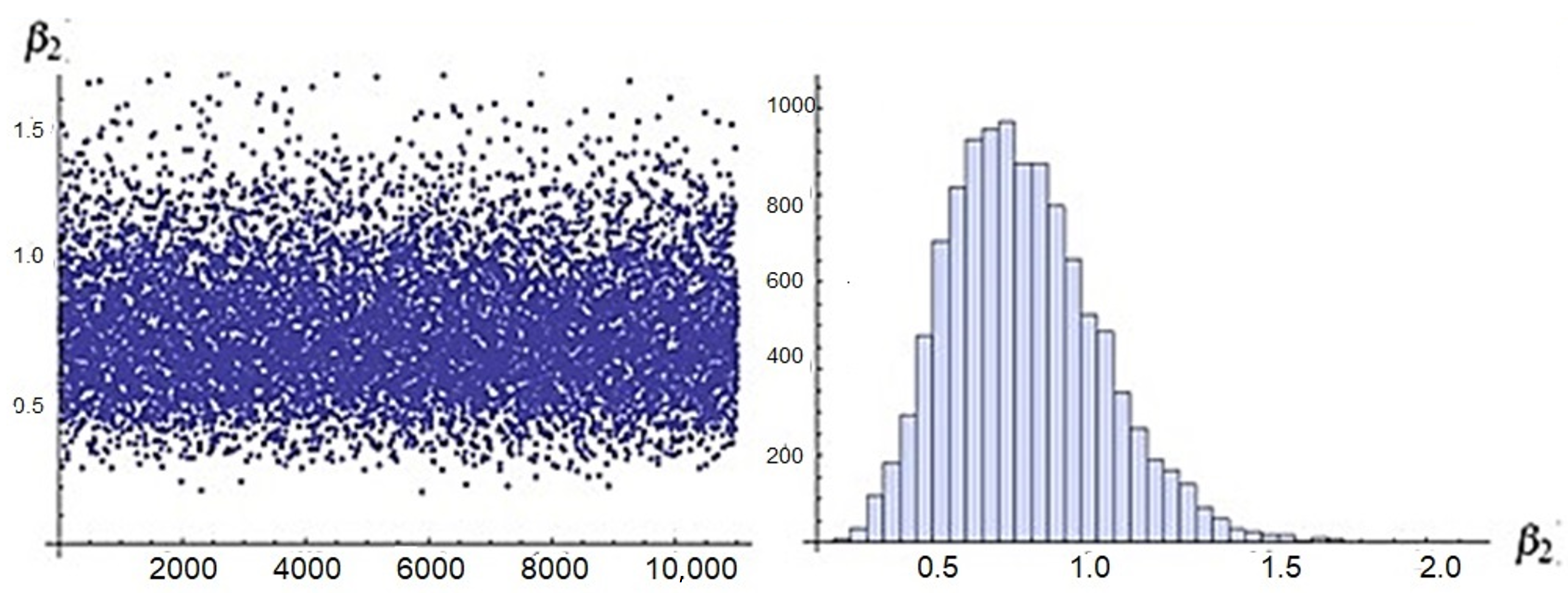
Figure 3, Figure 4, Figure 5 and Figure 6 show scatter plots of the model parameters generated by the MCMC method and the corresponding histograms, which showed the normality of posterior samples.

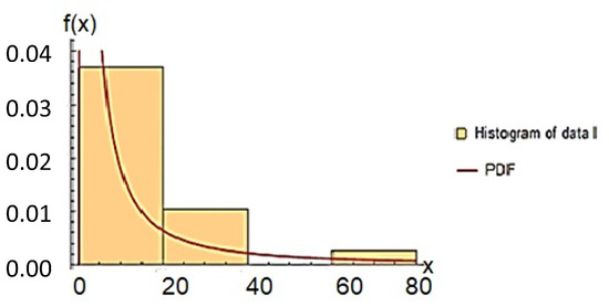
Figure 3. The estimate PDF of data 1.

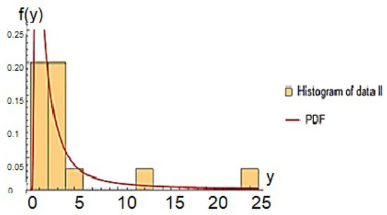
Figure 4. The estimate PDF of data 2.

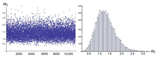
Figure 5. The scatter plot and the corresponding histogram of the parameter ${\alpha }_1$.

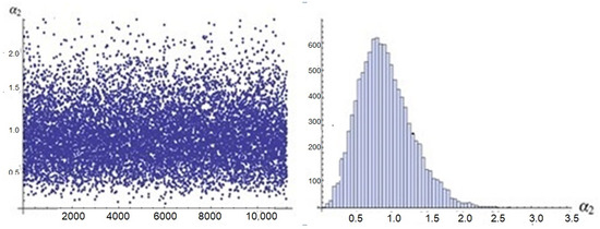
Figure 6. The scatter plot and the corresponding histogram of the parameter ${\alpha }_2$.

Results: From the numerical results, we observed some points, which can be described as follows:

1.

From the results presented in Table 1, Table 2, Table 3 and Table 4, adaptive type-II HPCS presents a more efficacious censoring scheme.

2.

In general, the MSE of all estimates decreases as the effective sample sizes increase.

3.

For all cases, the censoring scheme IV, in which the removed items after the first observed failure give more accurate results through the MSEs than the other schemes.

4.

Estimations under ML and non-informative Bayes are close to others.

5.

Bayesian estimation under informative prior information serves better than classical estimation (ML and bootstrapping) and non-informative Bayes estimation.

6.

The proposed model serves well for all of the parameter values.

7.

The informative Bayes credible interval serves better than bootstrap CIs and asymptotic CIs.

8.

As the effective sample sizes increase, the coverage probability for the parameters is close to the nominal level of 0.95.

9.

We also observed that better estimates are obtained by increasing the ideal test time $\tau$.

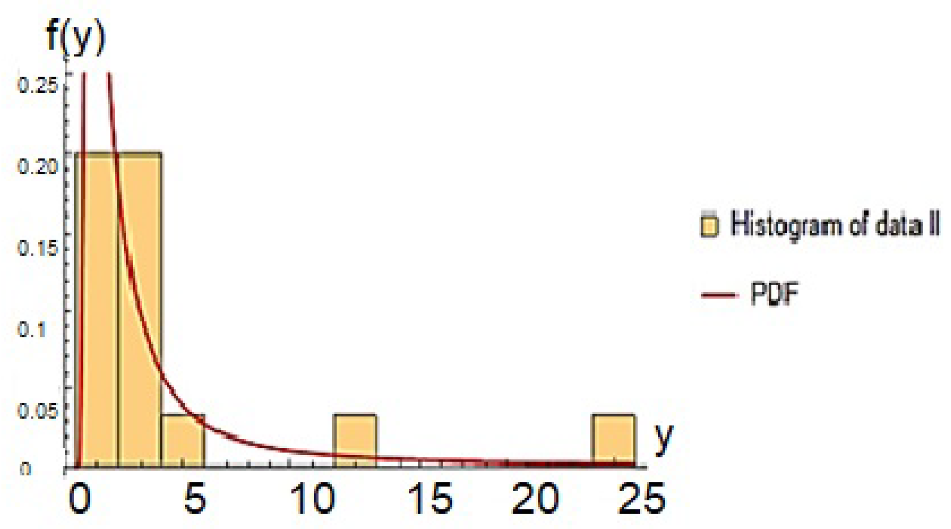
4.2. Real Data Example

In this section, we consider the combination of two real-life examples to illustrate and discuss the proposed model and the corresponding methods of estimation. The data were presented by Nelson [28] to describe breakdown times for insulating fluid per minute between two electrodes under different voltages. Data 1 was reported under 34. kilo-volts, and data 2 was reported under 36 kilo-volts. The data and the corresponding joint sample are presented in Table 5. The problem of fitting the data with respect to IWD was discussed by Alslman and Amal [29]. The estimate PDF of two data points is described in Figure 3 and Figure 4, see [29].

Table 5. The Breakdown times in minutes of insulating fluid Nelson [28].

Data 1	0.19, 0.78, 0.96, 1.31, 2.78, 3.16, 4.15, 4.67, 4.85, 6.5, 7.35, 8.01, 8.27, 12.06, 31.75,
	32.52, 33.91, 36.71, 72.89
Data 2	0.35, 0.59, 0.96, 0.99, 1.69, 1.97, 2.07, 2.58, 2.71, 2.9, 3.67, 3.99, 5.35, 13.77, 25.50
Joint data	(0.19,1), (0.35,0), (0.59,0), (0.78,1), (0.96,1), (0.96,0), (0.99,0), (1.31,1), (1.69,0), (1.97,0)
	(2.07,0), (2.58,0), (2.71,0), (2.78,1), (2.9,0), (3.16,1), (3.67,0), (3.99,0), (4.15,1)
	(4.67,1), (4.85,1), (5.35,2), (6.5,1), (7.35,1), (8.01,1), (8.27,1), (12.06,1), (13.77,0)
	(25.5,0), (31.75,1), (32.52,1), (33.91,1), (36.71,1), (72.89,1)
Joint adaptive	(0.19, 1), (0.35,0), (0.59,0), (0.78,1), (0.96,1), (0.96,0), (0.99,0), (1.69,0)
type-II HPCS	(1.97,0), (2.07,0), (3.16,1), (3.67,0), (3.99,0), (4.15,1), (4.67,1), (5.35,0), (7.35,1)
	(8.01,1), (13.77,0), (32.52,1), (33.91,1), (36.71,1)

Hence, we considered the IWD as a good fit for both data samples. From the joint sample, we generated the joint adaptive type-II PHCS under censoring scheme $\tau =10$ and $R=${1, 1, 1, 2, 1, 0, 0, 2, 0, 1, 0, 0, 1, 0, 0, 1, 0, 1, 0, 0, 0, 0}. The random generated sample and its type is reported in Table 5. The corresponding censoring schemes $R_1^{*}=${1, 0, 0, 1, 0, 0, 0, 1, 0, 1, 0, 0, 0, 0, 0, 0, 0, 1, 0, 0, 0, 0} and $R_1^{*}=${0, 1, 1, 1, 1, 0, 0, 1, 0, 0, 0, 0, 1, 0, 0, 1, 0, 0, 0, 0, 0, 0}. Point ML and Bayes estimates of the model parameters are reported in Table 6. The approximate confidence interval (ACI), bootstrap confidence intervals (BCI), and the Bayesian HP credible interval (HPCI) are computed and reported in Table 6. Estimations of reliability and failure rate functions of two lines are also computed, results are summarized in Table 7. In the Bayesian approach, we adopted non-informative prior information for the model parameters with values $a_i=b_i=0.0001$. For the MCMC approach, we ran the chain 11,000 times and discarded the first 1000 varieties as a burn-in. The MCMC trace and the associated histograms plots are displayed in Figure 5, Figure 6, Figure 7 and Figure 8. These figures show the convergence in the empirical posterior distribution.

Table 6. The point and 95% interval estimates of the parameters.

Pa.s	ML	Bayes	ACI	BCI	HPI
${\alpha }_1$	1.0222	1.6624	(0.2393, 1.8050)	(0.3412, 1.9925)	(0.6245, 1.7452)
${\alpha }_2$	0.5903	1.4963	(0.0603, 1.1202)	(0.1074, 1.3542)	(0.4215, 1.6542)
${\beta }_1$	0.7525	0.6135	(0.4103, 1.0947)	(0.4555, 1.4221)	(0.5008, 1.1245)
${\beta }_2$	1.5822	1.0196	(0.9066, 2.2578)	(0.9325, 2.4478)	(0.7421, 1.4582)

Table 7. Reliability and failure rate functions of two line for mission time $t=1.0$.

	${\mathit{S}}_1$	${\mathit{S}}_2$	${\mathit{h}}_1$	${\mathit{h}}_2$
ML	0.64018	0.445814	0.432319	1.16091
MCMC	0.793798	0.755609	0.246514	0.45368

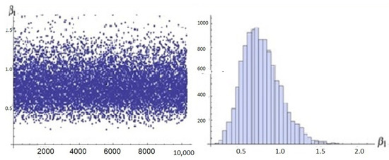
Figure 7. The scatter plot and the corresponding histogram of the parameter ${\beta }_1$.

Figure 8. The scatter plot and the corresponding histogram of the parameter ${\beta }_2$.

5. Conclusions

Comparative life tests have received a great deal of attention in recent years for industrial products that have many lines of manufacture within the same facility. In addition, there is difficulty determining the relative advantages of competing products in terms of competitive duration. So, in this study, we examined this problem for products from two production lines that have inverse Weibull lifetime distributions with different parameters. An adaptive type-II HPCS was proposed to reduce total test time and unit costs. For the unknown model parameters, both Bayesian and maximum likelihood techniques were used to estimate model parameters. The asymptotic confidence intervals were then computed using the observed information matrix. The bootstrap-P method can also be used to calculate confidence intervals. The Bayes estimates and credible intervals were computed using the Markov chain Monte Carlo method. Through Monte Carlo simulation studies, the developed methods were evaluated and compared. For all cases, the censoring scheme IV, in which the removed items were removed after the first observed failure, gives more accurate results through the MSEs than the other schemes. The HPD credible interval has the shortest interval length when compared to the ACI. The proposed model was tested using real-world data examples. The results obtained from this study indicate that the model and associated estimating methods work effectively in different cases. The current method can be extended to generate an ideal progressive censoring sampling plan.

References

- Liu, C.-C. A Comparison between the Weibull and Lognormal Models used to Analyze Reliability Data. Ph.D. Thesis, University of Nottingham, Nottingham, UK, 1997. [Google Scholar]
- Nelson, W. Applied Life Data Analysis; Wiley: New York, NY, USA, 1982; ISBN 0-471-09458-7. [Google Scholar]
- Cooray, K.; Gunasekera, S.; Ananda, M. Weibull and Inverse Weibull Composite Distribution for Modeling Reliability Data. Model Assist. Stat. Appl. 2010, 5, 109–115. [Google Scholar] [CrossRef]
- Nassar, M.; Abo-Kasem, O.E. Estimation of the inverse Weibull parameters under adaptive type-II progressive hybrid censoring scheme. J. Comput. Appl. Math. 2017, 315, 228–239. [Google Scholar] [CrossRef]
- Xu, R.; Gui, W. Entropy Estimation of InverseWeibull Distribution under Adaptive Type-II Progressive Hybrid Censoring Schemes. Symmmetry 2019, 11, 1463. [Google Scholar]
- Alkarni, S.; Afify, A.; Elbatal, I.; Elgarhy, M. The Extended Inverse Weibull Distribution: Properties and Applications. Complexity 2020, 2020, 3297693. [Google Scholar] [CrossRef]
- Balakrishnan, N.; Aggarwala, R. Progressive Censoring; Birkhauser: Boston, MA, USA, 2000. [Google Scholar]
- Balakrishnan, N. Progressive censoring methodology: An appraisal. Test 2007, 16, 211–259. [Google Scholar] [CrossRef]
- Ng, H.K.T.; Kundu, D.; Chan, P.S. Statistical analysis of exponential lifetimes under an adaptive Type-II progressive censoring scheme. Ceram. Int. 2009, 35, 237–246. [Google Scholar] [CrossRef]
- Abd-Elmougod, G.A.; El-Sayed, M.A.; Abdel-Rahman, E.O. Coefficient of variation of Topp-Leone distribution under adaptive Type-II progressive censoring scheme: Bayesian and non-Bayesian approach. J. Comput. Theor. 2015, 12, 4028–4035. [Google Scholar] [CrossRef]
- Bhattacharyya, G.K.; Mehrotra, K.G. On testing equality of two exponential distributions under combined type-IIcensoring. J. Am. Stat. Assoc. 1981, 6, 886–894. [Google Scholar] [CrossRef]
- Mehrotra, K.G.; Bhattacharyya, G.K. Confidence intervals with jointly type-II censored samples from two exponential distributions. J. Am. Stat. Assoc. 1982, 77, 441–446. [Google Scholar] [CrossRef]
- Balakrishnan, N.; Rasouli, A. Exact likelihood inference for two exponential populations under joint type-II censoring. Comput. Stat. Data Anal. 2008, 52, 2725–2738. [Google Scholar] [CrossRef]
- Rasouli, A.; Balakrishnan, N. Exact likelihood inference for two exponential populations under joint progressive type-II censoring. Commun. Stat. Theory Methods 2010, 39, 2172–2191. [Google Scholar] [CrossRef]
- Shafaya, A.R.; Balakrishnanbc, N.; Abdel-Atyd, Y. Bayesian inference based on a jointly type-II censored sample from two exponential populations. J. Stat. Comput. Simul. 2014, 84, 2427–2440. [Google Scholar] [CrossRef]
- Mondal, S.; Kundu, D. Bayesian Inference for Weibull Distribution under the Balanced Joint Type-II Progressive Censoring Scheme. Am. J. Math. Manag. Sci. 2019, 39, 56–74. [Google Scholar] [CrossRef]
- Algarni, A.; Almarashi, A.M.; Abd-Elmougod, G.A.; Abo-Eleneen, Z.A. Two compound Rayleigh lifetime distributions in analyses the jointly type-II censoring samples. J. Math. Chem. 2019, 58, 950–966. [Google Scholar] [CrossRef]
- Abushal, T.A.; Soliman, A.A.; Abd-Elmougod, G.A. Statistical inferences of Burr XII lifetime models under joint Type-1 competing risks samples. J. Math. 2021, 2021, 9553617. [Google Scholar] [CrossRef]
- Almarashi, A.M.; Algarni, A.; Daghistani, A.M.; Abd-Elmougod, G.A.; Abdel-Khalek, S.; Raqab, M.Z. Inferences for Joint Hybrid Progressive Censored Exponential Lifetimes under Competing Risk Model. Math. Probl. Eng. 2021, 2021, 3380467. [Google Scholar] [CrossRef]
- Shokr, E.M.; El-Sagheer, R.M.; Khder, M.; El-Desouky, B.S. Inferences for two Weibull Frechet populations under joint progressive type-II censoring with applications in engineering chemistry. Appl. Math. Inf. Sci. 2022, 16, 73–92. [Google Scholar]
- Tolba, A.H.; Abushal, T.A.; Ramadan, D.A. Statistical inference with joint progressive censoring for two populations using power Rayleigh lifetime distribution. Sci. Rep. 2023, 13, 3832. [Google Scholar] [CrossRef]
- Al-Essa, L.A.; Soliman, A.A.; Abd-Elmougod, G.A.; Alshanbari, H.M. Comparative Study with Applications for Gompertz Models under Competing Risks and Generalized Hybrid Censoring Schemes. Aximos 2023, 12, 322. [Google Scholar] [CrossRef]
- David, H.A.; Nagaraja, H.N. Order Statistics, 3rd ed.; Wiley: New York, NY, USA, 2003. [Google Scholar]
- Ng, H.K.T.; Chan, P.S. Comments on: Progressive censoring methodology: An appraisal. Test 2007, 16, 287–289. [Google Scholar] [CrossRef]
- Efron, B. The jackknife, the bootstrap and other resampling plans. In CBMS-NSF Regional Conference Series in Applied Mathematics; Monograph 38, SIAM: Phiadelphia, PA, USA, 1982. [Google Scholar]
- Chen, M.-H.; Shao, Q.-M. Monte Carlo estimation of Bayesian Credible and HPD intervals. J. Comput. Graph. Stat. 1999, 8, 69–92. [Google Scholar]
- Balakrishnan, N.; Sandhu, R.A. A simple simulation algorithm for generating progressively type-II censored samples. Am. Stat. 1995, 49, 229–230. [Google Scholar]
- Nelson, W.-B. Applied Life Data Analysis; John Wiley & Sons: Hoboken, NJ, USA, 2003; Volume 521. [Google Scholar]
- Alslman, M.; Helu, A. Estimation of the stress-strength reliability for the inverse Weibull distribution under adaptive type-II progressive hybrid censoring. PLoS ONE 2022, 8, e0277514. [Google Scholar] [CrossRef] [PubMed]
Disclaimer/Publisher’s Note: The statements, opinions and data contained in all publications are solely those of the individual author(s) and contributor(s) and not of MDPI and/or the editor(s). MDPI and/or the editor(s) disclaim responsibility for any injury to people or property resulting from any ideas, methods, instructions or products referred to in the content. |
© 2023 by the authors. Licensee MDPI, Basel, Switzerland. This article is an open access article distributed under the terms and conditions of the Creative Commons Attribution (CC BY) license (https://creativecommons.org/licenses/by/4.0/).