A Simplified Approach to the Pricing of Vulnerable Options with Two Underlying Assets in an Intensity-Based Model

Abstract

In this paper, we study a simplified approach to determine the pricing formula for vulnerable options involving two correlated underlying assets. We utilize an intensity-based model to describe the credit risk associated with these vulnerable options. Without the change of measure technique, we derive pricing formulas for vulnerable options involving two underlying assets based on the probabilistic approach. We provide closed-form pricing formulas for two specific types of options: the vulnerable exchange option and the vulnerable foreign equity option. Finally, we present numerical results to demonstrate the accuracy of our formulas using the Monte-Carlo method and the effect of various parameters on the price of options.

1. Introduction

The pricing problem of options with credit risk, also known as “vulnerable options”, has been extensively studied by numerous researchers. Vulnerable options are financial derivatives that take into account the credit risk of the counterparty. In general, two models have been used to model credit risk are the structural model and the intensity-based model. The structural model, proposed by Merton [1], Black and Cox [2] and Geske [3], depends on the option issuer’s firm value process. A credit event occurs in the structural model if the firm value process falls below the option issuer’s liability value at maturity. The intensity-based model, initially developed by Jarrow and Turnbull [4], Lando [5] and Jarrow and Yu [6], determines a credit event based on the jump of a Poisson process with a given intensity. In other words, the event is triggered by the first jump of the process, and there is no direct relationship between the option issuer’s value and the credit event.

The research on vulnerable options began primarily with a structural approach. As a result, the structural model has been used in many studies in the past to model credit risk in vulnerable option pricing. Credit events occur in the structural model when a firm’s asset value falls below a specified threshold. Johnson and Stulz [7] were the first to introduce a vulnerable European option pricing model in which the option is the counterparty’s sole liability. Klein [8] extended the results of Johnson and Stulz [7] by allowing the option writer to have other liabilities and providing a correlation between the underlying asset and the counterparty’s asset. Liao and Huang [9] considered the option issuer’s potential default during the remaining life of the option and developed pricing formulas for vulnerable options with stochastic interest rate. Jeon and Kim [10] used the Mellin transform approach to develop the works of [9] as two types of options. More recently, Wang [11], He et al. [12], Kim et al. [13] and Jeon et al. [14] investigated the pricing of vulnerable options in the presence of stochastic volatility affecting asset price processes. In addition, there have been numerous research on vulnerable options with multi-assets [15,16,17,18,19].

We utilize an intensity-based model to capture credit risk for this study since it is commonly used to evaluate the prices of credit derivatives such as credit default swaps (CDS) [20,21], defaultable bonds [22], total return swap (TRS) [23,24], and others. We use an intensity-based model to investigate the pricing of vulnerable options with multi-assets. There have recently been studies on vulnerable options within the framework of the intensity-based model. Fard [25] derived a pricing formula for vulnerable option under a generalized jump model and used an intensity-based model to account for counterparty credit risk. Wang [26] applied Generalized AutoRegressive Conditional Heteroskedasticity (GARCH) model for the underlying asset process and an intensity-based model for counterparty credit risk to obtain a solution for the price of vulnerable options under a discrete time model. Koo and Kim [27] chose an intensity-based model to capture the option issuer’s credit event and provided an explicit analytical valuation formula for a catastrophe put option with default risk using the multidimensional Girsanov theorem. Moreover, Pasricha and Goel [28] investigated a vulnerable power exchange option with two underlying assets within an intensity-based model using a doubly stochastic Poisson process to model the counterparty’s credit event and assuming correlation among the three underlying assets in both the continuous and jump components. Wang [29] derived explicit pricing formula for vulnerable Asian option within an intensity-based model when the underlying asset process follows a two-factor stochastic volatility model.

We present a simple method for pricing vulnerable options with two underlying assets within an intensity-based model in this paper,. Based on Fard’s model [25], we assume that the default intensity process, which is correlated with the underlying assets, follows a mean-reverting Ornstein-Uhlenbeck (OU) process. However, unlike Fard’s approach, we do not use the change of measure technique. Instead, we provide a simplified valuation method for pricing vulnerable options with correlated underlying assets that is based on the probabilistic approach. Using this proposed method, we derive closed-form pricing formulas for vulnerable exchange option and vulnerable foreign equity option in particular. Furthermore, we examine the accuracy of the formulas using the Monte Carlo (MC) simulation.

The rest of the paper is organized as follows. In Section 2, we introduce the underlying assets for pricing vulnerable options, along with an intensity-based model to account for credit risk. In Section 3, we provide the valuation formulas for vulnerable exchange options and vulnerable foreign equity options. Additionally, we introduce the lemmas used in option pricing. In Section 4, we carry out some numerical experiments to show the accuracy of our formulas obtained in Section 3. Finally, in Section 5, we present concluding remarks.

2. The Model

We assume that there are no arbitrage opportunities in the economy represented by a filtered complete probability space $(\Omega ,\mathcal{F},\{\mathcal{F}\left(t\right)\},Q)$ where Q is a risk-neutral probability measure and $\left\{\mathcal{F}\right(t\left)\right\}$ satisfies the usual conditions. Under the measure Q, the dynamics of two underlying assets are assumed to be

$$\begin{array}{ccc}& & d{S}_1\left(t\right)=r{S}_1\left(t\right)dt+{\sigma }_1{S}_1\left(t\right)d{W}_1\left(t\right),\hfill \\ & & d{S}_2\left(t\right)=r{S}_2\left(t\right)dt+{\sigma }_2{S}_2\left(t\right)d{W}_2\left(t\right),\hfill \end{array}$$

where r is a risk-free interest rate, ${\sigma }_i,(i=1,2)$ is volatility, and $W_1\left(t\right)$ and $W_2\left(t\right)$ are the correlated standard Brownian motions satisfying $d{W}_1\left(t\right)d{W}_2\left(t\right)={\rho }_{12}dt$. As in Fard [25], we assume that the process of default intensity is given by

$$\begin{array}{c}\hfill d\lambda \left(t\right)=a(b-\lambda \left(t\right))dt+{\sigma }_{3}d{W}_3\left(t\right),\end{array}$$

where $a,b$ and ${\sigma }_3$ are positive constants and $W_3\left(t\right)$ is the standard Brownian motion satisfying $d{W}_1\left(t\right)d{W}_3\left(t\right)={\rho }_{13}dt$ and $d{W}_2\left(t\right)d{W}_3\left(t\right)={\rho }_{23}dt$. With the process $\lambda \left(t\right)$, the default time $\tau$ of option issuer is defined by

$$\mathrm{P}(\tau >t)={\mathbf{E}}^Q\left[e^{-{\int }_0^t\lambda \left(s\right)ds}\right],t\in [0,T],$$

where T is the maturity and ${\mathrm{E}}^Q[·]$ denotes the expectation under the measure Q. Define ${\mathcal{F}}^{S_i}\left(t\right),(i=1,2)$ be the $\sigma$-field generated by the price processes of underlying asset $i,(i=1,2)$ such that ${\mathcal{F}}^{S_i}\left(t\right)=\sigma (S_i\left(s\right),s\le t),(i=1,2)$. Similarly, the filtration of the default intensity ${\mathcal{F}}^{\lambda }\left(t\right)$ and the filtration of the default time $\mathcal{H}\left(t\right)$ are defined as ${\mathcal{F}}^{\lambda }\left(t\right)=\sigma (\lambda \left(s\right),s\le t)$ and $\mathcal{H}\left(t\right)=\sigma ({\mathbf{1}}_{\{\tau \le s\}},s\le t)$, respectively. Then, the enlarged filtration $\mathcal{F}\left(t\right)$ is generated by $\mathcal{F}\left(t\right)={\mathcal{F}}^{S_1}\left(t\right)\vee {\mathcal{F}}^{S_2}\left(t\right)\vee {\mathcal{F}}^{\lambda }\left(t\right)\vee \mathcal{H}\left(t\right)$, where ${\mathbf{1}}_{\left\{\right\}}$ is the indicator function.

Let w be the recovery rate of the vulnerable option. Then, based on the results of Lando [5] and Fard [25], the price of vulnerable option with two underlying assets at time 0 in the intensity based model can be expressed as

$$\begin{array}{ccc}\hfill & & C=e^{-rT}{\mathbf{E}}^Q\left[w·h(S_1\left(T\right),S_2\left(T\right)){\mathbf{1}}_{\{\tau \le T\}}+h(S_1\left(T\right),S_2\left(T\right)){\mathbf{1}}_{\{\tau >T\}}|\mathcal{F}\left(0\right)\right]\hfill \\ & & =w{e}^{-rT}{\mathbf{E}}^Q\left[h(S_1\left(T\right),S_2\left(T\right))|\mathcal{F}\left(0\right)\right]\hfill \\ & & +(1-w)e^{-rT}{\mathbf{E}}^Q\left[e^{-{\int }_0^T\lambda \left(s\right)ds}h(S_1\left(T\right),S_2\left(T\right))|\mathcal{F}\left(0\right)\right],\hfill \end{array}$$

(1)

where $h(·,·)$ denotes the payoff function of option and w is a constant satisfying $0<w<1$.

3. The Valuation of Vulnerable Options with Two Underlying Assets

In this section, we present a simplified approach for pricing of vulnerable options with two underlying assets based on Equation (1). The proposed approach provides the option pricing formula without the method of changing measure. We now introduce the lemmas to obtain the pricing formulas.

Lemma 1.

Let $X_1$ and $X_2$ be random variables which have a bivariate normal distribution. Then, for any constant k,

$$\mathbf{E}\left[e^{X_1}{\mathbf{1}}_{\{X_2\ge k\}}\right]=e^{\mathbf{E}\left[X_1\right]+\frac{\mathbf{Var}\left[X_1\right]}{2}}\mathbf{N}\left(\frac{\mathbf{Cov}(X_1,X_2)+\mathbf{E}\left[X_2\right]-k}{\sqrt{\mathbf{Var}\left[X_2\right]}}\right),$$

where $\mathbf{Var}$ is the variance operator, $\mathbf{Cov}$ is the covariance operator and $\mathbf{N}$ is the cumulative standard normal distribution function.

Proof. 

For convenience, we write expectations and variances of random variables as

$$\mathbf{E}\left[X_1\right]={\mu }_1,\mathbf{Var}\left[X_1\right]={\sigma }_1^2,\mathbf{E}\left[X_2\right]={\mu }_2,\mathbf{Var}\left[X_2\right]={\sigma }_2^2,$$

respectively.

By the conditional distribution of $X_1$ given $X_2$ and the moment generating functions of normal variables, we have

$$\begin{array}{ccc}\hfill \mathbf{E}\left[e^{X_1}{\mathbf{1}}_{\{X_2\ge k\}}\right]& =& \mathbf{E}\left[\mathbf{E}\left[e^{X_1}\right|X_2]{\mathbf{1}}_{\{X_2\ge k\}}\right]\hfill \\ & =& \mathbf{E}\left[e^{{\mu }_1+\rho \frac{{\sigma }_1}{{\sigma }_2}(X_2-{\mu }_2)+\frac{1}{2}{\sigma }_1^2(1-{\rho }^2)}{\mathbf{1}}_{\{X_2\ge k\}}\right]\hfill \\ & =& e^{{\mu }_1-\rho \frac{{\sigma }_1}{{\sigma }_2}{\mu }_2+\frac{1}{2}{\sigma }_1^2(1-{\rho }^2)}\mathbf{E}\left[e^{\rho \frac{{\sigma }_1}{{\sigma }_2}{X}_2}{\mathbf{1}}_{\{X_2\ge k\}}\right],\hfill \end{array}$$

where k is some constant and $\rho$ is the correlation between $X_1$ and $X_2$. Then, by the change of variable $X_2={\mu }_2+{\sigma }_2{Z}_2$, we have

$$\begin{array}{ccc}\hfill \mathbf{E}\left[e^{\rho \frac{{\sigma }_1}{{\sigma }_2}{X}_2}{\mathbf{1}}_{\{X_2\ge k\}}\right]& =& e^{\rho \frac{{\sigma }_1}{{\sigma }_2}{\mu }_2}\mathbf{E}\left[e^{\rho {\sigma }_1{Z}_2}{\mathbf{1}}_{\{Z_2\ge \frac{k-{\mu }_2}{{\sigma }_2}\}}\right]\hfill \\ & =& e^{\rho \frac{{\sigma }_1}{{\sigma }_2}{\mu }_2+\frac{1}{2}{\rho }^2{\sigma }_1^2}{\int }_{\frac{k-{\mu }_2}{{\sigma }_2}}^{\infty }\frac{e^{-\frac{1}{2}{(Z_2-\rho {\sigma }_1)}^2}}{\sqrt{2\pi }}d{Z}_2.\hfill \end{array}$$

This completes the proof. □

Lemma 2.

Let $X_1,X_2$ and $X_3$ be random variables which have a trivariate normal distribution. Then,

$$\mathbf{E}\left[e^{-X_3}g(X_1,X_2)\right]=\mathbf{E}\left[e^{-X_3}\right]\mathbf{E}[g(X_1-\mathbf{Cov}(X_1,X_3),X_2-\mathbf{Cov}(X_2,X_3)],$$

for which the expectations exist for any function $g(·,·)$.

Proof. 

Let us define the function $\hat{f}$ such that

$$\hat{f}(x_1,x_2):={\int }_{-\infty }^{\infty }{e}^{-x_3}f(x_1,x_2,x_3)d{x}_3,$$

where f is the joint density function of $(X_1,X_2,X_3)$. Then, we have

$$\begin{array}{ccc}& & \mathbf{E}\left[e^{-X_3}g(X_1,X_2)\right]\hfill \\ & & ={\int }_{-\infty }^{\infty }{\int }_{-\infty }^{\infty }{\int }_{-\infty }^{\infty }{e}^{-x_3}g(x_1,x_2)f(x_1,x_2,x_3)d{x}_{1}d{x}_{2}d{x}_3\hfill \\ & & ={\int }_{-\infty }^{\infty }{\int }_{-\infty }^{\infty }g(x_1,x_2)\hat{f}(x_1,x_2)d{x}_{1}d{x}_2.\hfill \end{array}$$

We now consider the moment generating function (MGF) of $(X_1,X_2,X_3)$. That is, MGF of $(X_1,X_2,X_3)$ is given by $\varphi (s,t,u)=\mathbf{E}\left[e^{s{X}_1+t{X}_2+u{X}_3}\right]$. If $g(x_1,x_2)=e^{x_1+x_2}$, we can find that

$$\varphi (s,t,-1)=\mathbf{E}\left[e^{s{X}_1+t{X}_2-X_3}\right]={\int }_{-\infty }^{\infty }{\int }_{-\infty }^{\infty }{e}^{s{x}_1+t{x}_2}\hat{f}(x_1,x_2)d{x}_{1}d{x}_2.$$

Here, $s{X}_1+t{X}_2-X_3$ has a normal distribution. It follows that

$$\begin{array}{ccc}& & \varphi (s,t,-1)\hfill \\ & & =exp\left(s\mathbf{E}\left[X_1\right]+t\mathbf{E}\left[X_2\right]-\mathbf{E}\left[X_3\right]+\frac{s^2\mathbf{Var}\left[X_1\right]}{2}+\frac{t^2\mathbf{Var}\left[X_2\right]}{2}+\frac{\mathbf{Var}\left[X_3\right]}{2}\right.\hfill \\ & & \left.+st\mathbf{Cov}[X_1,X_2]-t\mathbf{Cov}[X_2,X_3]-s\mathbf{Cov}[X_1,X_3]\right)\hfill \\ & & =e^{-\mathbf{E}\left[X_3\right]+\frac{\mathbf{Var}\left[X_3\right]}{2}}\hfill \\ & & \times exp\left(s(\mathbf{E}\left[X_1\right]-\mathbf{Cov}[X_1,X_3])+\frac{s^2\mathbf{Var}\left[X_1\right]}{2}\right.\hfill \\ & & \left.+t(\mathbf{E}\left[X_2\right]-\mathbf{Cov}[X_2,X_3])+\frac{t^2\mathbf{Var}\left[X_2\right]}{2}+st\mathbf{Cov}[X_1,X_2]\right)\hfill \\ & & =\mathbf{E}\left[e^{-X_3}\right]\mathbf{E}[exp\left(s(X_1-\mathbf{Cov}[X_1,X_3])+t(X_2-\mathbf{Cov}[X_2,X_3])\right)].\hfill \end{array}$$

Since MGF uniquely determines the distribution, $\hat{f}(x_1,x_2)/\mathbf{E}\left[e^{-X_3}\right]$ becomes a density function of $(X_1-\mathbf{Cov}[X_1,X_3],X_2-\mathbf{Cov}[X_2,X_3])$. Therefore, we conclude that

$$\begin{array}{c}\hfill \mathbf{E}\left[e^{-X_3}g(X_1,X_2)\right]=\mathbf{E}\left[e^{-X_3}\right]{\int }_{-\infty }^{\infty }{\int }_{-\infty }^{\infty }g(x_1,x_2)\frac{\hat{f}(x_1,x_2)}{\mathbf{E}\left[e^{-X_3}\right]}d{x}_{1}d{x}_2.\end{array}$$

This completes the proof. □

We investigate the pricing of vulnerable options with two underlying assets under the intensity based model using Lemmas 1 and 2. Specifically, we deal with two kinds of options: vulnerable foreign equity option and vulnerable exchange option, and derive the closed-form pricing formulas of the options.

3.1. Vulnerable Exchange Option

Margrabe [30] first derived the closed-form pricing formula of the european exchange option which provides the option holder the right to exchange one risky asset for another. Since its introduction by Margrabe [30], the option has become one of the most popular exotic options in the over-the-counter (OTC) market. We assume that the dynamics of underlying assets and default intensity follow the processes defined in the previous section. From Equation (1), the vulnerable exchange option price at time 0 with maturity T is given by

$$\begin{array}{ccc}\hfill V\left(0\right)& =& (1-w)e^{-rT}{\mathbf{E}}^Q\left[e^{-{\int }_0^T\lambda \left(s\right)ds}{(S_1\left(T\right)-S_2\left(T\right))}^{+}|\mathcal{F}\left(0\right)\right]\hfill \\ & & +w{e}^{-rT}{\mathbf{E}}^Q\left[{(S_1\left(T\right)-S_2\left(T\right))}^{+}|\mathcal{F}\left(0\right)\right]\hfill \\ & :=& (1-w)e^{-rT}{V}_1+w{e}^{-rT}{V}_2.\hfill \end{array}$$

(2)

Then, using the Lemmas 1 and 2, we can derive the closed-form pricing formula of vulnerable exchange option in the intensity based model.

Theorem 1.

The price of vulnerable exchange option at time 0 is given by

$$\begin{array}{ccc}& & V\left(0\right)=(1-w){\Lambda }_1\left(S_1\left(0\right)e^{-\frac{{\sigma }_1{\sigma }_3{\rho }_{13}}{a}{\int }_0^{T}u(s,T,a)ds}\mathbf{N}\left(d_1\right)-S_2\left(0\right)e^{-\frac{{\sigma }_2{\sigma }_3{\rho }_{23}}{a}{\int }_0^{T}u(s,T,a)ds}\mathbf{N}\left(d_2\right)\right)\hfill \\ & & +w\left(S_1\left(0\right)\mathbf{N}\left({\hat{d}}_1\right)-S_2\left(0\right)\mathbf{N}\left({\hat{d}}_2\right)\right),\hfill \end{array}$$

(3)

where

$$\begin{array}{ccc}& & d_1=\frac{ln\left(\frac{S_1\left(0\right)}{S_2\left(0\right)}\right)+\frac{1}{2}{\sigma }^{2}T+\left(\frac{{\sigma }_2{\sigma }_3{\rho }_{23}-{\sigma }_1{\sigma }_3{\rho }_{13}}{a}\right){\int }_0^{T}u(s,T,a)ds}{\sigma \sqrt{T}},\hfill \\ & & d_2=d_1-\sigma \sqrt{T},\hfill \\ & & {\hat{d}}_1=\frac{ln\left(\frac{S_1\left(0\right)}{S_2\left(0\right)}\right)+\frac{1}{2}{\sigma }^{2}T}{\sigma \sqrt{T}},\hfill \\ & & {\hat{d}}_2={\hat{d}}_1-\sigma \sqrt{T},\hfill \\ & & {\Lambda }_1=exp\left[-bT-\frac{\lambda \left(0\right)-b}{a}(1-e^{-aT})+\frac{{\sigma }_3^2}{2a^2}{\int }_0^T{u}^2(s,T,a)ds\right],\hfill \\ & & u(s,T,a)=1-e^{-a(T-s)},\hfill \\ & & {\sigma }^2={\sigma }_1^2+{\sigma }_2^2-2{\rho }_{12}{\sigma }_1{\sigma }_2.\hfill \end{array}$$

Proof. 

Using Lemma 2, we can decompose $V_1$ into two expectations as follows.

$$\begin{array}{ccc}\hfill V_1& =& {\mathbf{E}}^Q\left[e^{-{\int }_0^T\lambda \left(s\right)ds}{(S_1\left(T\right)-S_2\left(T\right))}^{+}|\mathcal{F}\left(0\right)\right]\hfill \\ & =& e^{-bT-\frac{\lambda \left(0\right)-b}{a}(1-e^{-aT})}{\mathbf{E}}^Q\left[e^{-X_3}|\mathcal{F}\left(0\right)\right]\hfill \\ & & \times {\mathbf{E}}^Q\left[g(X_1-\mathbf{Cov}(X_1,X_3),X_2-\mathbf{Cov}(X_2,X_3))|\mathcal{F}\left(0\right)\right],\hfill \end{array}$$

(4)

where $X_1={\sigma }_1{W}_1\left(T\right),X_2={\sigma }_2{W}_2\left(T\right),X_3=\frac{{\sigma }_3}{a}{\int }_0^{T}u(s,T,a)d{W}_3\left(s\right)$ and

$$g(x,y)={(S_1\left(0\right)e^{(r-\frac{1}{2}{\sigma }_1^2)T+x}-S_2\left(0\right)e^{(r-\frac{1}{2}{\sigma }_2^2)T+y})}^{+}.$$

Using the Ito isometry, we find that the random variable $X_3$ is normally distributed with mean 0 and variance $\frac{{\sigma }_3^2}{a^2}{\int }_0^T{u}^2(s,T,a)ds$. Then, the first expectation in Equation (4) can be calculated easily. Next, let us consider the second expectation in Equation (4). The expectation can be represented by

$$\begin{array}{ccc}\hfill & & {\mathbf{E}}^Q\left[g(X_1-\mathbf{Cov}(X_1,X_3),X_2-\mathbf{Cov}(X_2,X_3))|\mathcal{F}\left(0\right)\right]\hfill \\ & & =S_1\left(0\right)e^{(r-\frac{1}{2}{\sigma }_1^2)T-\frac{{\sigma }_1{\sigma }_3{\rho }_{13}}{a}{\int }_0^{T}u(s,T,a)ds}\hfill \\ & & \times {\mathbf{E}}^Q\left[e^{X_1}{\mathbf{1}}_{\{S_1\left(T\right)e^{-\mathbf{Cov}(X_1,X_3)}>S_2\left(T\right)e^{-\mathbf{Cov}(X_2,X_3)}\}}|\mathcal{F}\left(0\right)\right]\hfill \\ & & -S_2\left(0\right)e^{(r-\frac{1}{2}{\sigma }_2^2)T-\frac{{\sigma }_2{\sigma }_3{\rho }_{23}}{a}{\int }_0^{T}u(s,T,a)ds}\hfill \\ & & \times {\mathbf{E}}^Q\left[e^{X_2}{\mathbf{1}}_{\{S_1\left(T\right)e^{-\mathbf{Cov}(X_1,X_3)}>S_2\left(T\right)e^{-\mathbf{Cov}(X_2,X_3)}\}}|\mathcal{F}\left(0\right)\right].\hfill \end{array}$$

(5)

$X_1-X_2$ is normally distributed with mean 0 and variance ${\sigma }^{2}T$. Then, by applying Lemma 1, we can calculate two expectations in Equation (5).

$$\begin{array}{ccc}& & {\mathbf{E}}^Q\left[e^{X_i}{\mathbf{1}}_{\{S_1\left(T\right)e^{-\mathbf{Cov}(X_1,X_3)}>S_2\left(T\right)e^{-\mathbf{Cov}(X_2,X_3)}\}}|\mathcal{F}\left(0\right)\right]=e^{\frac{{\sigma }_i^2}{2}T}\mathbf{N}\left(d_i\right),fori=1,2.\hfill \end{array}$$

This completes the formula for $V_1$. Finally, since $V_2$ is Margrabe’s formula which is well known, we can obtain the pricing formula for vulnerable exchange option. □

Remark 1.

Theorem 1 is also applicable to the vulnerable european options in the intensity based model. The vulnerable european call option price can be obtained by setting strike $K=S_2\left(0\right)e^{rT}$ and ${\sigma }_2=0$.

3.2. Vulnerable Foreign Equity Option

Foreign equity options are contingent claims where the payoffs are determined by underlying assets in one currency, but the actual payoff is converted to another currency at maturity. Following Kwok [31], there are four types of foreign equity options. Among them, we consider a foreign equity option call stuck in domestic currency in this paper.

Let $S_f\left(t\right)$ and $S_d\left(t\right)$ be the asset price in foreign currency and the asset price in domestic currency, respectively. We denote the exchange rate specified in domestic currency per unit of the foreign currency at time t by $Y\left(t\right)$, so that the relation between $S_f\left(t\right)$ and $S_d\left(t\right)$ is formulated as $S_d\left(t\right)=Y\left(t\right)S_f\left(t\right)$. We also assume that $r_d$ and $r_f$ are the domestic and foreign risk-free interest rates, respectively. As shown by Kwok and Wong [32] and Martzoukos [33], under risk-neutral probability measure Q, the price processes for $S_f\left(t\right)$ and $S_d\left(t\right)$ are given by

$$\begin{array}{ccc}& & d{S}_d\left(t\right)=(r_d-q)S_d\left(t\right)dt+{\sigma }_1{S}_d\left(t\right)d{W}_1\left(t\right),\hfill \\ & & d{S}_f\left(t\right)=(r_f-q-{\rho }_{12}{\sigma }_1{\sigma }_2)S_f\left(t\right)dt+{\sigma }_1{S}_f\left(t\right)d{W}_1\left(t\right),\hfill \end{array}$$

where q is the dividend of the asset, ${\sigma }_1$ is the volatility of the asset and $W_1\left(t\right)$ is the standard Brownian motion, respectively. Also, the exchange rate process $Y\left(t\right)$ is given by

$$dY\left(t\right)=(r_d-r_f)Y\left(t\right)dt+{\sigma }_{2}Y\left(t\right)d{W}_2\left(t\right),$$

where ${\sigma }_2$ is the volatility of exchange rate and $W_2\left(t\right)$ is the standard Brownian motion satisfying $d{W}_1\left(t\right)d{W}_2\left(t\right)={\rho }_{12}dt$ under the measure Q. Then, with the process of default intensity $\lambda \left(t\right)$ defined in the previous section, a vulnerable foreign equity option call price in domestic currency at time 0 with domestic strike K and maturity T is given by

$$\begin{array}{ccc}\hfill C\left(0\right)& =& (1-w)e^{-r_{d}T}{\mathbf{E}}^Q\left[e^{-{\int }_0^T\lambda \left(s\right)ds}{(Y\left(T\right)S_f\left(T\right)-K)}^{+}|\mathcal{F}\left(0\right)\right]\hfill \\ & & +w{e}^{-r_{d}T}{\mathbf{E}}^Q\left[{(Y\left(T\right)S_f\left(T\right)-K)}^{+}|\mathcal{F}\left(0\right)\right]\hfill \\ & :=& (1-w)e^{-r_{d}T}{C}_1+w{e}^{-r_{d}T}{C}_2.\hfill \end{array}$$

(6)

We present the closed-form pricing formula of vulnerable foreign equity option in the the following theorem.

Theorem 2.

The price of vulnerable foreign equity option at time 0 is given by

$$\begin{array}{ccc}& & C\left(0\right)=(1-w){\Lambda }_1\hfill \\ & & \times \left(Y\left(0\right)S_f\left(0\right)e^{(-q+\frac{1}{2}{\sigma }_f^2)T-\left(\frac{{\sigma }_2{\sigma }_3{\rho }_{23}+{\sigma }_1{\sigma }_3{\rho }_{13}}{a}\right){\int }_0^{T}u(s,T,a)ds}\mathbf{N}\left(d_1\right)-K{e}^{-r_{d}T}\mathbf{N}\left(d_2\right)\right)\hfill \\ & & +w\left(Y\left(0\right)S_f\left(0\right)e^{-qT}\mathbf{N}\left({\hat{d}}_1\right)-K{e}^{-r_{d}T}\mathbf{N}\left({\hat{d}}_2\right)\right),\hfill \end{array}$$

(7)

where $u(s,T,a)$ and ${\Lambda }_1$ are defined in Theorem 1, and

$$\begin{array}{ccc}& & d_1=\frac{ln\left(\frac{Y\left(0\right)S_f\left(0\right)}{K}\right)+\left(r_d-q+\frac{1}{2}{\sigma }_f^2\right)T-\left(\frac{{\sigma }_2{\sigma }_3{\rho }_{23}+{\sigma }_1{\sigma }_3{\rho }_{13}}{a}\right){\int }_0^{T}u(s,T,a)ds}{{\sigma }_f\sqrt{T}},\hfill \\ & & {\hat{d}}_1=\frac{ln\left(\frac{Y\left(0\right)S_f\left(0\right)}{K}\right)+\left(r_d-q+\frac{1}{2}{\sigma }_f^2\right)T}{{\sigma }_f\sqrt{T}},\hfill \\ & & d_2=d_1-{\sigma }_f\sqrt{T},\hfill \\ & & {\hat{d}}_2={\hat{d}}_1-{\sigma }_f\sqrt{T},\hfill \\ & & {\sigma }_f^2={\sigma }_1^2+{\sigma }_2^2+2{\rho }_{12}{\sigma }_1{\sigma }_2.\hfill \end{array}$$

Proof. 

Similar to Theorem 1, applying Lemma 2, we can rewrite $C_1$ as

$$\begin{array}{ccc}\hfill C_1& =& {\mathbf{E}}^Q\left[e^{-{\int }_0^T\lambda \left(s\right)ds}{(Y\left(T\right)S_f\left(T\right)-K)}^{+}|\mathcal{F}\left(0\right)\right]\hfill \\ & =& e^{-bT-\frac{\lambda \left(0\right)-b}{a}(1-e^{-aT})}{\mathbf{E}}^Q\left[e^{-X_3}|\mathcal{F}\left(0\right)\right]\hfill \\ & & \times {\mathbf{E}}^Q\left[g(X_1-\mathbf{Cov}(X_1,X_3),X_2-\mathbf{Cov}(X_2,X_3))|\mathcal{F}\left(0\right)\right],\hfill \end{array}$$

(8)

where $X_1={\sigma }_1{W}_1\left(T\right),X_2={\sigma }_2{W}_2\left(T\right),X_3=\frac{{\sigma }_3}{a}{\int }_0^{T}u(s,T,a)d{W}_3\left(s\right)$, and

$$g(x,y)={(Y\left(0\right)S_f\left(0\right)e^{(r_d-q-\frac{1}{2}{\sigma }_f^2)T+x+y}-K)}^{+}.$$

The first expectation in Equation (8) can be calculated easily, and the second expectation can be represented by

$$\begin{array}{ccc}\hfill & & {\mathbf{E}}^Q\left[g(X_1-\mathbf{Cov}(X_1,X_3),X_2-\mathbf{Cov}(X_2,X_3))|\mathcal{F}\left(0\right)\right]\hfill \\ & & =Y\left(0\right)S_f\left(0\right)e^{(r_d-q-\frac{1}{2}{\sigma }_f^2)T-\left(\frac{{\sigma }_2{\sigma }_3{\rho }_{23}+{\sigma }_1{\sigma }_3{\rho }_{13}}{a}\right){\int }_0^{T}u(s,T,a)ds}\hfill \\ & & \times {\mathbf{E}}^Q\left[e^{X_1+X_2}{\mathbf{1}}_{\{Y\left(T\right)S_f\left(T\right)e^{-\left(\frac{{\sigma }_2{\sigma }_3{\rho }_{23}+{\sigma }_1{\sigma }_3{\rho }_{13}}{a}\right){\int }_0^{T}u(s,T,a)ds}>K\}}|\mathcal{F}\left(0\right)\right]\hfill \\ & & -K{\mathbf{E}}^Q\left[{\mathbf{1}}_{\{Y\left(T\right)S_f\left(T\right)e^{-\left(\frac{{\sigma }_2{\sigma }_3{\rho }_{23}+{\sigma }_1{\sigma }_3{\rho }_{13}}{a}\right){\int }_0^{T}u(s,T,a)ds}>K\}}|\mathcal{F}\left(0\right)\right].\hfill \end{array}$$

(9)

Since $X_1+X_2$ is normally distributed with mean 0 and variance ${\sigma }_f^{2}T$, the second expectation in Equation (9) is

$$\begin{array}{ccc}& & {\mathbf{E}}^Q\left[{\mathbf{1}}_{\{Y\left(T\right)S_f\left(T\right)e^{-\left(\frac{{\sigma }_2{\sigma }_3{\rho }_{23}+{\sigma }_1{\sigma }_3{\rho }_{13}}{a}\right){\int }_0^{T}u(s,T,a)ds}>K\}}|\mathcal{F}\left(0\right)\right]\hfill \\ & & ={\mathbf{P}}^Q\left(Y\left(T\right)S_f\left(T\right)>K{e}^{\left(\frac{{\sigma }_2{\sigma }_3{\rho }_{23}+{\sigma }_1{\sigma }_3{\rho }_{13}}{a}\right){\int }_0^{T}u(s,T,a)ds}|\mathcal{F}\left(0\right)\right)\hfill \\ & & ={\mathbf{P}}^Q\left(-X_1-X_2\right.\hfill \\ & & \left.<ln\left(\frac{Y\left(0\right)S_f\left(0\right)}{K}\right)+\left(r_d-q+\frac{1}{2}{\sigma }_f^2\right)T-\left(\frac{{\sigma }_2{\sigma }_3{\rho }_{23}+{\sigma }_1{\sigma }_3{\rho }_{13}}{a}\right){\int }_0^{T}u(s,T,a)ds\right)\hfill \\ & & =\mathbf{N}\left(d_2\right).\hfill \end{array}$$

In Equation (9), the expectations can be calculated using Lemma 1. Moreover, $C_2$ can be calculated easily without the use of Lemma 2. Finally, we obtain the pricing formula combining above results . □

Remark 2.

As in Fard [25], the pricing formulas in Theorems 1 and 2 can be derived using the change of measure method. However, in the intensity based model, the approach based on Lemma 1 and Lemma 2 is simpler for pricing vulnerable options with two underlying assets.

4. Numerical Experiments

In this section, we present numerical experiments that demonstrate the impact of significant parameters on the option price and verify the accuracy of our pricing formulas. We specifically compare the pricing formula values with the option values generated using the Monte Carlo (MC) simulation method, and we provide graphs for illustrating the sensitivity analysis of parameters on the vulnerable options.

4.1. Monte Carlo Simulation

In this subsection, we show the accuracy of our approach by comparing the values by the pricing formulas in the previous section and those MC simulations with 20,000 sample paths and 500 time steps.

Using the Euler discretization, the sample paths of the processes for vulnerable exchange option are given by

$$\begin{array}{ccc}& & ln{S}_1(t+\Delta t)=ln{S}_1\left(t\right)+(r-0.5{\sigma }_1^2)\Delta t+{\sigma }_1\sqrt{\Delta t}{\epsilon }_1,\hfill \\ & & ln{S}_2(t+\Delta t)=ln{S}_2\left(t\right)+(r-0.5{\sigma }_2^2)\Delta t+{\sigma }_2\sqrt{\Delta t}({\rho }_{12}{\epsilon }_1+\sqrt{1-{\rho }_{12}^2}{\epsilon }_2),\hfill \\ & & \lambda (t+\Delta t)=\lambda \left(t\right)+a(b-\lambda \left(t\right))\Delta t+{\sigma }_3\sqrt{\Delta t}({\rho }_{13}{\epsilon }_1+\widehat{{\rho }_{23}}{\epsilon }_2+\sqrt{1-{\rho }_{13}^2-{\widehat{{\rho }_{23}}}^2}{\epsilon }_3),\hfill \end{array}$$

where $\Delta t=1/1000$, $\widehat{{\rho }_{23}}=({\rho }_{23}-{\rho }_{12}{\rho }_{13})/\sqrt{1-{\rho }_{12}^2}$, and ${\epsilon }_1,{\epsilon }_2,{\epsilon }_3$ are identical and independent samples from the standard normal distribution with mean 0 and variance 1. The experiments’ default parameters for the vulnerable exchange option price are $S_1\left(0\right)=S_2\left(0\right)=100,r=0.03,T=1,\lambda \left(0\right)=0.45,{\sigma }_1=0.18,{\sigma }_2=0.12,{\sigma }_3=0.25,{\rho }_{12}={\rho }_{13}={\rho }_{23}=1,a=0.06,b=1.5$ and $w=0.75$.

The values $V\left(0\right)$ by Theorem 1 and the values using MC method are shown in

Table 1. Price of vulnerable exchange option. All experiments are conducted using the MATLAB.

			Vulnerable Exchange Option
${\mathit{S}}_{\mathbf{1}}\left(\mathbf{0}\right)$	${\mathit{S}}_{\mathbf{2}}\left(\mathbf{0}\right)$	$\mathit{w}$	Price  $\mathit{V}\left(\mathbf{0}\right)$	Monte Carlo	R-Err
100	60	0.25	27.763	28.185	1.52$\times {10}^{-2}$
		0.5	31.842	31.496	1.08$\times {10}^{-2}$
		0.75	35.921	35.908	3.53$\times {10}^{-4}$
	80	0.25	13.716	13.738	1.67$\times {10}^{-3}$
		0.5	15.811	15.801	6.01$\times {10}^{-4}$
		0.75	17.905	17.974	3.89$\times {10}^{-3}$
	100	0.25	1.519	1.545	1.71$\times {10}^{-2}$
		0.5	1.811	1.839	1.54$\times {10}^{-2}$
		0.75	2.102	2.117	7.37$\times {10}^{-3}$
Av. run time (s)			0.031	18.1211

. The values of ‘R-err’ in Table 1 are the relative error between values by the pricing formulas and values by the MC method defined by

$$\mathrm{R}-\mathrm{err}\triangleq \left|\frac{\mathrm{Value}\mathrm{by}\mathrm{formula}-\mathrm{Value}\mathrm{by}\mathrm{MC}}{\mathrm{Value}\mathrm{by}\mathrm{formula}}\right|.$$

The results in Table 1 demonstrate that our option pricing formula is accurate. Furthermore, we find that experiments with the proposed pricing formula take less than 0.1 s on average while the Monte Carlo simulations take almost 20 s on average.

Table 2. Price of vulnerable foreign equity option. All experiments are conducted using the MATLAB.

			Vulnerable Foreign Equity Option
${\mathit{S}}_{\mathit{f}}\left(\mathbf{0}\right)$	$\mathit{K}$	$\mathit{w}$	Price $\mathit{C}\left(\mathbf{0}\right)$	Monte Carlo	R-Err
100	60	0.25	37.211	37.067	3.87$\times {10}^{-3}$
		0.5	42.120	42.454	7.93$\times {10}^{-3}$
		0.75	47.019	46.960	1.24$\times {10}^{-3}$
	80	0.25	24.480	24.418	2.53$\times {10}^{-3}$
		0.5	27.665	27.677	4.39$\times {10}^{-4}$
		0.75	30.849	30.850	1.929$\times {10}^{-5}$
	100	0.25	14.332	14.344	8.50$\times {10}^{-4}$
		0.5	16.179	16.159	1.21$\times {10}^{-3}$
		0.75	18.028	17.984	2.41$\times {10}^{-3}$
Av. run time (s)			0.030	18.2574

provides comparison of vulnerable foreign equity option values calculated through our formula given in Theorem 2 and values obtained through the MC method. The processes of the vulnerable foreign equity option are discretized similarly to the processes of vulnerable exchange option. Table 2 shows the accuracy of our formula, as expected. The experiments’ default parameters for the vulnerable foreign equity option price are $S_f\left(0\right)=100,K=100,Y\left(0\right)=1.1,r_d=r_f=0.03,T=1,q=0,\lambda \left(0\right)=0.45,{\sigma }_1=0.18,$ ${\sigma }_2=0.12,{\sigma }_3=0.25,{\rho }_{12}={\rho }_{13}={\rho }_{23}=1,a=0.06,b=1.5$ and $w=0.75$.

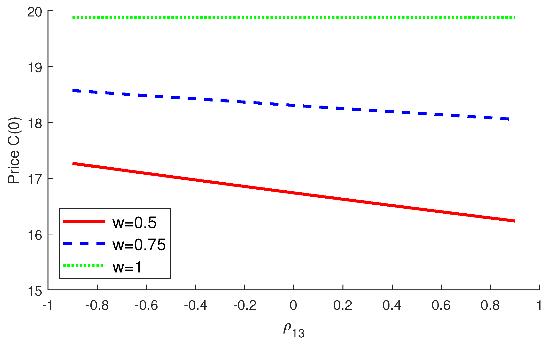
4.2. Numerical Examples

Figure 1, Figure 2, Figure 3, Figure 4, Figure 5 and Figure 6 illustrate the vulnerable exchange option prices in the intensity-based model to investigate the impact of various parameters. Figure 1 and Figure 2 present the option prices against maturity T for three recovery rate parameters $w=0.5,0.75,1$ and initial intensity parameters $\lambda \left(0\right)=0.5,1.5,2.5$. From Figure 1 and Figure 2, we observe that option price increases when the maturity increases. As expected, in Figure 1, we can find that a lager value of w corresponds a higher price of option. We also find that option the prices decrease with an increase in $\lambda \left(0\right)$ in Figure 2. Figure 3 displays option prices against volatility ${\sigma }_1$ of underlying asset $S_1\left(t\right)$ for three maturities $T=0.5,1,1.5$. From Figure 3, we observe that option prices increase for ${\sigma }_1>1.2$, but decrease for ${\sigma }_1<1.2$ for all maturity. In Figure 4, we report option prices against volatility ${\sigma }_3$ of intensity process. Since the probability of default increases as ${\sigma }_3$ increases, the prices decrease with an increase in ${\sigma }_3$. Figure 5 and Figure 6 show the option prices against the correlations ${\rho }_{12}$ and ${\rho }_{13}$ respectively and for three recovery rate parameters. We observe that the option prices decrease when the correlation ${\rho }_{12}$ increases. This is because two underlying assets $S_1\left(t\right)$ and $S_2\left(t\right)$ move in the same direction for positive correlation. Different from Figure 5, the price is constant for $w=1$. This is due to the fact that the correlation ${\rho }_{13}$ does not have any role because credit risk does not occur when $w=1$. If $w\ne 1$, the prices decrease as ${\rho }_{13}$ increases.

Figure 7, Figure 8, Figure 9, Figure 10, Figure 11 and Figure 12 illustrate the vulnerable foreign equity option prices in the intensity-based model to investigate the impact of various parameters. In most of the Figures, except for Figure 9, we can see that the behaviors of foreign equity option prices are similar to the behaviors of exchange option prices for same parameters. In contrast to Figure 3, in Figure 9, as ${\sigma }_1$ x increases, the option prices also increase continuously. This is due to the difference in the structure of the payoff function.

5. Concluding Remarks

In this paper, we investigate a simple approach for pricing vulnerable options with two correlated underlying assets in an intensity-based model. The mean-reverting OU process, which is correlated with the underlying assets, is used to model credit risk. We obtain option pricing formulas using the properties of three random variables without changing the measure. The approach presented in this study is easily expanded to more general vulnerable options in the intensity-based model. We derive closed-form pricing formulas for two types of options with two underlying assets using the proposed approach: exchange option and and foreign equity option. Finally, we provide numerical results using the MC simulation method to show the accuracy of our option pricing formula and graphs to illustrate the impacts of different parameters on option price.

This study employs the mean-reverting OU process for stochastic intensity based on Fard’s model [25], however it has a limitation: the intensity cannot be negative mathematically, but the mean-reverting OU process for intensity can have negative values. To overcome this problem, stochastic intensity models that do not allow negative values, such as the CIR model, should be used to vulnerable option pricing in the intensity-based model. This will be studied further in the future via the change of measure method.

References

1. Merton, R.C. On the pricing of corporate debt: The risk structure of interest rates. J. Financ. 1974, 29, 449–470. [Google Scholar]
2. Black, F.; Cox, J.C. Valuing corporate securities: Some effects of bond indenture provisions. J. Financ. 1976, 31, 351–367. [Google Scholar] [CrossRef]
3. Geske, R. The valuation of corporate liabilities as compound options. J. Financ. Quant. Anal. 1977, 12, 541–552. [Google Scholar] [CrossRef]
4. Jarrow, R.; Turnbull, S. Pricing options on financial securities subject to default risk. J. Financ. 1995, 50, 53–86. [Google Scholar] [CrossRef]
5. Lando, D. On Cox processes and credit risky securities. Rev. Deriv. Res. 1998, 2, 99–120. [Google Scholar] [CrossRef]
6. Jarrow, R.A.; Yu, F. Counterparty risk and the pricing of defaultable securities. J. Financ. 2001, 56, 1765–1799. [Google Scholar] [CrossRef]
7. Johnson, H.; Stulz, R. The pricing of options with default risk. J. Financ. 1987, 42, 267–280. [Google Scholar] [CrossRef]
8. Klein, P. Pricing Black-Scholes options with correlated credit risk. J. Bank. Financ. 1996, 20, 1211–1229. [Google Scholar] [CrossRef]
9. Liao, S.L.; Huang, H.H. Pricing Black–Scholes options with correlated interest rate risk and credit risk: An extension. Quant. Financ. 2005, 5, 443–457. [Google Scholar] [CrossRef]
10. Jeon, J.; Kim, G. Pricing of vulnerable options with early counterparty credit risk. N. Am. J. Econ. Financ. 2019, 47, 645–656. [Google Scholar] [CrossRef]
11. Wang, X. Analytical valuation of Asian options with counterparty risk under stochastic volatility models. J. Futur. Mark. 2020, 40, 410–429. [Google Scholar] [CrossRef]
12. He, W.H.; Wu, C.; Gu, J.W.; Ching, W.K.; Wong, C.W. Pricing vulnerable options under a jump-diffusion model with fast mean-reverting stochastic volatility. J. Ind. Manag. Optim. 2022, 18, 2077–2094. [Google Scholar] [CrossRef]
13. Kim, D.; Choi, S.Y.; Yoon, J.H. Pricing of vulnerable options under hybrid stochastic and local volatility. Chaos Solitons Fractals 2021, 146, 110846. [Google Scholar] [CrossRef]
14. Jeon, J.; Huh, J.; Kim, G. An analytical approach to the pricing of an exchange option with default risk under a stochastic volatility model. Adv. Contin. Discret. Model. 2023, 2023, 37. [Google Scholar] [CrossRef]
15. Kim, G. Valuation of Exchange Option with Credit Risk in a Hybrid Model. Mathematics 2020, 8, 2091. [Google Scholar] [CrossRef]
16. Wang, X. Valuing vulnerable options with two underlying assets. Appl. Econ. Lett. 2020, 27, 1699–1706. [Google Scholar] [CrossRef]
17. Kim, D.; Yoon, J.H.; Kim, G. Closed-form pricing formula for foreign equity option with credit risk. Adv. Differ. Equations 2021, 2021, 1–17. [Google Scholar] [CrossRef]
18. Jeon, J.; Kim, G. Power Exchange Option with a Hybrid Credit Risk under Jump-Diffusion Model. Mathematics 2021, 10, 53. [Google Scholar] [CrossRef]
19. Dong, Z.; Tang, D.; Wang, X. Pricing vulnerable basket spread options with liquidity risk. Rev. Deriv. Res. 2023, 26, 23–50. [Google Scholar] [CrossRef]
20. Jamshidian, F. Valuation of credit default swaps and swaptions. Financ. Stochastics 2004, 8, 343–371. [Google Scholar] [CrossRef]
21. Leung, S.Y.; Kwok, Y.K. Credit default swap valuation with counterparty risk. Kyoto Econ. Rev. 2005, 74, 25–45. [Google Scholar]
22. Zhang, J.; Bi, X.; Li, R.; Zhang, S. Pricing credit derivatives under fractional stochastic interest rate models with jumps. J. Syst. Sci. Complex. 2017, 30, 645–659. [Google Scholar] [CrossRef]
23. Wang, A.; Ye, Z. Total return swap valuation with counterparty risk and interest rate risk. Abstr. Appl. Anal. 2014, 12, 412890. [Google Scholar] [CrossRef]
24. Wang, A. The pricing of total return swap under default contagion models with jump-diffusion interest rate risk. Indian J. Pure Appl. Math. 2020, 51, 361–373. [Google Scholar] [CrossRef]
25. Fard, F.A. Analytical pricing of vulnerable options under a generalized jump–diffusion model. Insur. Math. Econ. 2015, 60, 19–28. [Google Scholar] [CrossRef]
26. Wang, X. Analytical valuation of vulnerable options in a discrete-time framework. Probab. Eng. Informational Sci. 2017, 31, 100–120. [Google Scholar] [CrossRef]
27. Koo, E.; Kim, G. Explicit formula for the valuation of catastrophe put option with exponential jump and default risk. Chaos Solitons Fractals 2017, 101, 1–7. [Google Scholar] [CrossRef]
28. Pasricha, P.; Goel, A. Pricing vulnerable power exchange options in an intensity based framework. J. Comput. Appl. Math. 2019, 355, 106–115. [Google Scholar] [CrossRef]
29. Wang, X. Analytical valuation of vulnerable European and Asian options in intensity-based models. J. Comput. Appl. Math. 2021, 393, 113412. [Google Scholar] [CrossRef]
30. Margrabe, W. The value of an option to exchange one asset for another. J. Financ. 1978, 33, 177–186. [Google Scholar] [CrossRef]
31. Kwok, Y.K. Mathematical Models of Financial Derivatives; Springer: Berlin, Germany, 2008. [Google Scholar]
32. Kwok, Y.K.; Wong, H.Y. Currency-translated foreign equity options with path dependent features and their multi-asset extensions. Int. J. Theor. Appl. Financ. 2000, 3, 257–278. [Google Scholar] [CrossRef]
33. Martzoukos, S.H. Contingent claims on foreign assets following jump-diffusion processes. Rev. Deriv. Res. 2003, 6, 27–45. [Google Scholar] [CrossRef]
Figure 1. Price of vulnerable exchange option against T for recovery rates w = 0.5 , 0.75 , 1 .
Axioms 12 01105 g001
Figure 2. Price of vulnerable exchange option against T for initial intensities λ ( 0 ) = 0.5 , 1.5 , 2.5 .
Axioms 12 01105 g002
Figure 3. Price of vulnerable exchange option against σ 1 for maturities T = 0.5 , 1 , 1.5 .
Axioms 12 01105 g003
Figure 4. Price of vulnerable exchange option against σ 3 for maturities T = 0.5 , 1 , 1.5 .
Axioms 12 01105 g004
Figure 5. Price of vulnerable exchange option against ρ 12 for recovery rates w = 0.5 , 0.75 , 1 .
Axioms 12 01105 g005
Figure 6. Price of vulnerable exchange option against ρ 13 for recovery rates w = 0.5 , 0.75 , 1 .
Axioms 12 01105 g006
Figure 7. Price of vulnerable foreign equity option against T for recovery rates w = 0.5 , 0.75 , 1 .
Axioms 12 01105 g007
Figure 8. Price of vulnerable foreign equity option against T for initial intensities λ ( 0 ) = 0.5 , 1.5 , 2.5 .
Axioms 12 01105 g008
Figure 9. Price of vulnerable foreign equity option against σ 1 for maturities T = 0.5 , 1 , 1.5 .
Axioms 12 01105 g009
Figure 10. Price of vulnerable foreign equity option against σ 3 for maturities T = 0.5 , 1 , 1.5 .
Axioms 12 01105 g010
Figure 11. Price of vulnerable foreign equity option against ρ 12 for recovery rates w = 0.5 , 0.75 , 1 .
Axioms 12 01105 g011
Figure 12. Price of vulnerable foreign equity option against ρ 13 for recovery rates w = 0.5 , 0.75 , 1 .
Axioms 12 01105 g012