Analysis of the Burgers–Huxley Equation Using the Nondimensionalisation Technique: Universal Solution for Dirichlet and Symmetry Boundary Conditions

Abstract

The Burgers–Huxley equation is important because it involves the phenomena of accumulation, drag, diffusion, and the generation or decay of species, which are common in various problems in science and engineering, such as heat transmission, the diffusion of atmospheric contaminants, etc. On the other hand, the mathematical technique of nondimensionalisation has proven to be very useful in the appropriate grouping of the variables involved in a physical–chemical phenomenon and in obtaining universal solutions to different complex engineering problems. Therefore, a deep analysis using this technique of the Burgers–Huxley equation and its possible boundary conditions can facilitate a common understanding of these problems through the appropriate grouping of variables and propose common universal solutions. Thus, in this case, the technique is applied to obtain a universal solution for Dirichlet and symmetric boundary conditions. The validation of the methodology is carried out by comparing different cases, where the coefficients or the value of the boundary condition are varied, with the results obtained through a numerical simulation. Furthermore, one of the cases presented presents a boundary condition that changes at a certain time. Finally, after applying the technique, it is studied which phenomenon is predominant, concluding that from a certain value diffusion predominates, with the rest being practically negligible.

1. Introduction

Many engineering problems, such as heat transmission, fluid mechanics, contaminant emission, chloride diffusion in concrete, etc., involve the phenomena of diffusion, accumulation, generation, or the decay of species, and drag. In this sense, the Burgers–Huxley equation is a general equation that encompasses all these phenomena [1,2,3,4,5,6,7,8,9,10,11,12,13,14,15,16,17,18,19,20,21,22,23,24,25,26,27,28].

Thus, it is necessary, on the one hand, to obtain a universal solution that allows this equation to be easily solved, and on the other, to study the influence of the variables involved. In this way, the nondimensionalisation technique allows us to both obtain universal solutions and study the variables that have been grouped to form monomials [29,30,31].

The application of the nondimensionalisation technique to engineering problems formulated in ordinary differential equations is well known because it allows one to obtain dimensionless groups by grouping the variables, allowing us to know both the universal solution of the problem and the influence of each variable [31]. This procedure has recently been applied to different engineering problems, such as the diffusion of chlorides in concrete or soil consolidation, and the basis of the methodology has been explained in detail [29,31].

The objective of this study is to apply the nondimensionalisation methodology to the Burgers–Huxley equation to obtain, on the one hand, a universal solution to the problem posed. In this case, the symmetry condition will be applied to one of the boundary conditions, and to the other boundary condition, a constant value of the variable will be applied (Dirichlet condition). On the other hand, another objective is to study the weight of the variables in the problem. For the construction of the universal curves, the Network Simulation Method was used, which has demonstrated its effectiveness in solving this problem, as well as other engineering problems [32,33,34,35].

Thus, the Burgers–Huxley equation is an ordinary differential equation that is widely used in physics, biology, economics, etc., and includes terms such as drag, accumulation, generation or decay, and diffusion. This equation has the following form [2,3,32]:

$$\frac{du}{dt}+\alpha u^{\delta }\frac{du}{dx}-\zeta \frac{d^{2}u}{d{x}^2}-\beta u\left(1-u^{\delta }\right)\left(\epsilon u^{\delta }-\gamma \right)=0t\ge 0$$

(1)

where u is the variable, such as concentration, temperature, etc.; x is the distance; t is the time; and, finally, α, β, γ, δ, ε, and ζ are coefficients. Thus, the first addend of the equation is associated with accumulation, the second with drag (coefficients α and δ), the third with diffusion phenomena (coefficient ζ), and, finally, the fourth with the generation or decay of species (coefficients β, γ, δ, and ε).

This article is structured as follows: the introduction and the Burgers–Huxley equation are presented in Section 1. In the next section, the procedure for the nondimensionalisation technique is detailed so that it can be applied to the Burgers–Huxley equation in the same section. The results used to validate the proposed methodology after the application of the nondimensionalisation technique are presented in Section 3. Finally, Section 4 presents the conclusions of this study.

2. Nondimensionalisation Technique and Its Application to the Burgers–Huxley Equation

The correct steps for applying the nondimensionalisation technique have been described in the literature, which have recently included those necessary to obtain universal solutions. Furthermore, several articles have focused on defining the behaviour of monomials based on the values obtained, establishing criteria in which some monomials can have little influence on the problem compared with others that govern it. Thus, as a summary, the following steps must be applied [30,31]:

(i)

Choice of references

For the correct choice of references, a deep understanding of the problem is necessary because they may appear explicitly in the problem or may be hidden. Furthermore, the values selected for the references are related to each other through a physical interval (temporal or spatial) of the independent variable, limiting the dimensionless variables to the interval of values [0–1]. When the solution to the problem is asymptotic, references close to the limit are taken as the dependent variable, for example, 99% or 90% of the maximum value of the variable. Thus, there was no significant modification in the range [0–1] of the dimensionless variables.

(ii)

Dimensionless variables and dimensionless governing equations

The divisions between the dimensional variables and their references are the dimensionless variables, e.g., $x^{\prime }=\frac{x}{L}$, where x’ is the dimensionless variable of the distance, x is the distance variable, and L is the reference, which in this case is the total length of the medium. Thus, these dimensionless variables are introduced into the governing equations of the problem and transform them into dimensionless equations. Each addend of these equations is formed by two factors: one that involves the grouping of boundary conditions, problem parameters, and/or references, and another with dimensionless variables and their changes, which can be assumed to be of the order of unity. Thus, based on this hypothesis, the first factor, known as the coefficient, must also be of the same order of magnitude.

(iii)

Dimensionless groups

The dimensionless groups, or monomials, are the relation between the coefficients mentioned in the previous step, which will be at most as many addends as the dimensionless equation has minus one. Because some groups may be expressed as a combination of other groups with multiplications or divisions, or the same group may appear in more than one equation when the problem is a system of coupled equations, the final number of groups may be reduced. Additionally, the groups can be manipulated such that each unknown appears in a single group.

(iv)

The existence of m groups with a different unknown each one (π_u) and n groups without unknowns (π_w)

The solution for each unknown is explicitly expressed as a function of groups that do not contain unknowns. That is, in the form

$${\pi }_{u,i}={\Psi }_i\left({\pi }_{w,1},{\pi }_{w,2},\dots ,{\pi }_{w,n} \right) where 1\le i\le m$$

(2)

where Ψ_i is an arbitrary function of the n π_w groups. When the groups are of unit order of magnitude, the arbitrary function will also be of this order of magnitude.

(v)

Functionals

The Ψ_i functionals presented in the previous step were obtained by adjusting two monomials or dimensionless groups, keeping the rest at a constant value, as will be shown in the resolution of the problem posed in this article.

(vi)

Universal solutions

The universal solution is obtained by representing the dimensionless variables defined above, which, as indicated by their own definition, are in the range of values [0–1].

The information provided above is very important because it allows us to both obtain universal solutions to the problem posed and know the influence of the variables on it. Thus, if we apply this methodology to the Burgers–Huxley equation, we can obtain its universal solution and study the influence of its variables.

The study problem must be defined before applying the nondimensionalisation methodology. In this case, we have a variable u that is found in a medium of length L and is subject to the accumulation, drag, generation or decay, and diffusion phenomena. Regarding the boundary conditions, on the left side, a Dirichlet condition is applied with a constant value of u, u_ext, and on the right side, there is a Neumann condition to apply with a symmetry condition [32]. Finally, the variable u can present initial values in the medium, u_ini, as shown in Figure 1.

To apply the steps specified above for correct nondimensionalisation to Equation (1), the references must first be defined, and the dimensionless variables must be established (steps i and ii). Thus, dimensionless variables are the division of the variable with its reference.

$$u^{\prime }=\frac{u-u_{ini}}{u_{ext}-u_{ini}} x^{\prime }=\frac{x}{L} t^{\prime }=\frac{t}{\tau }$$

(3)

The reference chosen for the dimensionless variable u’ is the difference between the final value it can reach, that is, the value in the boundary condition, u_ext, and its initial value, u_ini. For the dimensionless variable x’, the total length of the medium, L, was chosen. Finally, because the problem has an asymptotic tendency, for the dimensionless time variable t’, the time at which 99% of the maximum value of u is reached, that is, 99% of u_ext, was chosen. The dimensionless variables were then introduced into the governing equation and the following dimensionless form was obtained:

$$\begin{gathered} \left[\frac{u_{ext}-u_{ini}}{\tau }\right]\frac{d{u}^{\prime }}{d{t}^{\prime }}+\alpha {\left(\left(u_{ext}-u_{ini}\right)u^{\prime }+u_{ini}\right)}^{\delta }\frac{u_{ext}-u_{ini}}{L}\frac{d{u}^{\prime }}{d{x}^{\prime }}-\left[\zeta \frac{u_{ext}-u_{ini}}{L^2}\right]\frac{d^2{u}^{\prime }}{d{x^{\prime }}^2}-\beta \epsilon {\left(\left(u_{ext}-u_{ini}\right)u^{\prime }+u_{ini}\right)}^{\delta +1}+ \\ \beta \gamma \left(\left(u_{ext}-u_{ini}\right)u^{\prime }+u_{ini}\right)+\beta \epsilon {\left(\left(u_{ext}-u_{ini}\right)u^{\prime }+u_{ini}\right)}^{2\delta +1}-\beta \gamma {\left(\left(u_{ext}-u_{ini}\right)u^{\prime }+u_{ini}\right)}^{\delta +1}=0. \end{gathered}$$

(4)

The dimensionless equation gives us seven coefficients:

$$\frac{u_{ext}-u_{ini}}{\tau }, \frac{\alpha u_{ext}^{\delta }\left(u_{ext}-u_{ini}\right)}{L}, \zeta \frac{u_{ext}-u_{ini}}{L^2}, \beta \epsilon u_{ext}^{\delta +1}, \beta \gamma u_{ext}, \beta \epsilon u_{ext}^{2\delta +1}, \beta \gamma u_{ext}^{\delta +1}.$$

As some coefficients of species generation or decay phenomena are contained in the others, there are finally five coefficients:

$$\frac{{\mathrm{u}}_{\mathrm{e}\mathrm{x}\mathrm{t}}-{\mathrm{u}}_{\mathrm{i}\mathrm{n}\mathrm{i}}}{\mathsf{\tau }},\frac{\mathsf{\alpha }{\mathrm{u}}_{\mathrm{e}\mathrm{x}\mathrm{t}}^{\mathsf{\delta }}\left({\mathrm{u}}_{\mathrm{e}\mathrm{x}\mathrm{t}}-{\mathrm{u}}_{\mathrm{i}\mathrm{n}\mathrm{i}}\right)}{\mathrm{L}},\mathsf{\zeta }\frac{{\mathrm{u}}_{\mathrm{e}\mathrm{x}\mathrm{t}}-{\mathrm{u}}_{\mathrm{i}\mathrm{n}\mathrm{i}}}{{\mathrm{L}}^2},\mathsf{\beta }\mathsf{\epsilon }{\mathrm{u}}_{\mathrm{e}\mathrm{x}\mathrm{t}}^{2\mathsf{\delta }+1},\mathsf{\beta }\mathsf{\gamma }{\mathrm{u}}_{\mathrm{e}\mathrm{x}\mathrm{t}}^{\mathsf{\delta }+1}.$$

These give rise to four dimensionless monomials:

$${\pi }_1=\frac{\zeta \tau }{L^2},\hspace{1em}\hspace{1em}{\pi }_2=\frac{\zeta }{\alpha L{u}_{ext}^{\delta }},\hspace{1em}\hspace{1em}{\pi }_3=\frac{\beta \gamma L{u}_{ext}}{\alpha \left(u_{ext}-u_{ini}\right)},\hspace{1em}\hspace{1em}{\pi }_4=\frac{\epsilon }{\gamma }{u}_{ext}^{\delta }.$$

The first monomial, π₁, is typical of problems involving diffusion phenomena, relating time to the distance squared and the diffusion coefficient, in this case, coefficient ζ. This monomial is found in the literature on heat transmission problems, known as the Fourier number [9], chloride diffusion [29], etc. The second monomial, π₂, indicates the relationship between diffusion and drag phenomena. The third, π₃, relates to the drag phenomena and the generation or decay of species. Finally, π₄ relates the coefficients of generation and decay of the species. It should be noted that when β is zero, the monomial π₃ is zero, and the fourth monomial π₄ has no influence, since there would be no generation or decay of the species.

Applying the π theorem, ${\pi }_1=\Psi \left({\pi }_2,{\pi }_3,{\pi }_4 \right)$, the same characteristic time can be expressed from each of the equations in the form

$$\tau =\frac{L^2}{\zeta }\Psi \left(\frac{\zeta }{\alpha L{u}_{ext}^{\delta }},\frac{\beta \gamma L{u}_{ext}}{\alpha \left(u_{ext}-u_{ini}\right)}, \frac{\epsilon }{\gamma }{u}_{ext}^{\delta } \right).$$

(5)

where Ψ is an unknown function of the arguments.

If we apply step (v) of the nondimensionalisation technique, the value of the functional can be obtained. In this case, because we depend on three monomials, we adjust the monomials π₁ and π₂, keeping the rest, π₃ and π₄, with constant values. To perform the adjustment, the problem was simulated using the Network Simulation Method to determine the time necessary for the concentration at the right-hand end, $x=L$, to be 99% of the u_ext value, as defined above. Thus, Equations (6)–(10) show the fits for different values of π₃ and π₄.

$${\pi }_3=0\hspace{1em} \forall {\pi }_4\hspace{1em}{\pi }_1=1.974+0.8186{{\pi }_2}^{-1.105}\hspace{1em}{\mathrm{R}}^2=0.9987\hspace{1em}\tau =\frac{L^2}{\zeta }\left(1.974+0.8186{\left(\frac{\zeta }{\alpha L{u}_{ext}^{\delta }}\right)}^{-1.105}\right)$$

(6)

$${\pi }_3=1\hspace{1em}{\pi }_4=1\hspace{1em}{\pi }_1=1.974+0.6781{{\pi }_2}^{-1.13}\hspace{1em}{\mathrm{R}}^2=0.9978\hspace{1em}\tau =\frac{L^2}{\zeta }\left(1.974+0.6781{\left(\frac{\zeta }{\alpha L{u}_{ext}^{\delta }}\right)}^{-1.13}\right)$$

(7)

$${\pi }_3=1\hspace{1em}{\pi }_4=2\hspace{1em}{\pi }_1=2.284+9708{{\pi }_2}^{-13.33}\hspace{1em}{\mathrm{R}}^2=1.0000\hspace{1em}\tau =\frac{L^2}{\zeta }\left(2.284+9708{\left(\frac{\zeta }{\alpha L{u}_{ext}^{\delta }}\right)}^{-13.33}\right)$$

(8)

$${\pi }_3=2\hspace{1em}{\pi }_4=1\hspace{1em}{\pi }_1=1.978+0.562{{\pi }_2}^{-1.102}\hspace{1em}{\mathrm{R}}^2=0.9990\hspace{1em}\tau =\frac{L^2}{\zeta }\left(1.978+0.562{\left(\frac{\zeta }{\alpha L{u}_{ext}^{\delta }}\right)}^{-1.102}\right)$$

(9)

$${\pi }_3=2\hspace{1em}{\pi }_4=2\hspace{1em}{\pi }_1=2.290+4674{{\pi }_2}^{-12.32}\hspace{1em}{\mathrm{R}}^2=1.0000\hspace{1em}\tau =\frac{L^2}{\zeta }\left(2.290+4674{\left(\frac{\zeta }{\alpha L{u}_{ext}^{\delta }}\right)}^{-12.32}\right)$$

(10)

As can be seen, in Equations (6)–(10), the R² fits are very close to unity. It should be noted that for Equation (6) β takes zero and, therefore, the monomial π₄ has no influence. Finally, Figure 2 shows the fit of Equations (6)–(10).

If the expressions obtained and Figure 2 are analysed, it can be seen that for very low values of π₂, very high values of π₁ are required, showing a tendency towards infinity. This indicates that the diffusion phenomenon is practically negligible, and with the drag phenomenon, it would be very difficult to reach a value of 99% of u_ext. This trend increased with increasing π₄, as shown in Figure 2. Owing to this tendency, the values provided by the fits for π₂ values lower than unity may have a higher error. On the other hand, for all the cases studied, from when π₂ takes a value between two and five, π₁ tends to be a value close to two, becoming practically independent of π₂, π₃, and π₄; therefore, the diffusion phenomenon governs the problem, as shown in Figure 2.

Finally, if step (vi) is applied by simulating the problem using the Network Simulation Method [32], and presenting u’ versus x’ for different values of t’, the universal solution to the problem is obtained, as shown in Figure 3.

The methodology for using the universal solution to obtain the value of u at a given position and time is as follows.

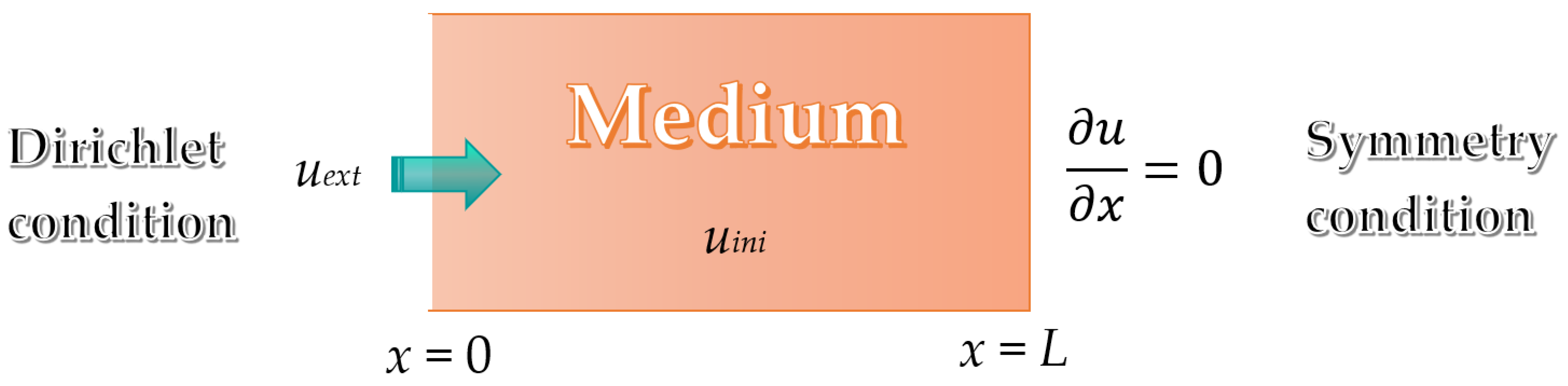
• The values of position x and time t at which the u value is to be determined are known. In addition, the value of u at the boundary condition, u_ext, the initial value of u at position x, u_ini, and the length of the medium, L, are known. In addition, the coefficients α, β, γ, δ, ε, and ζ are known.
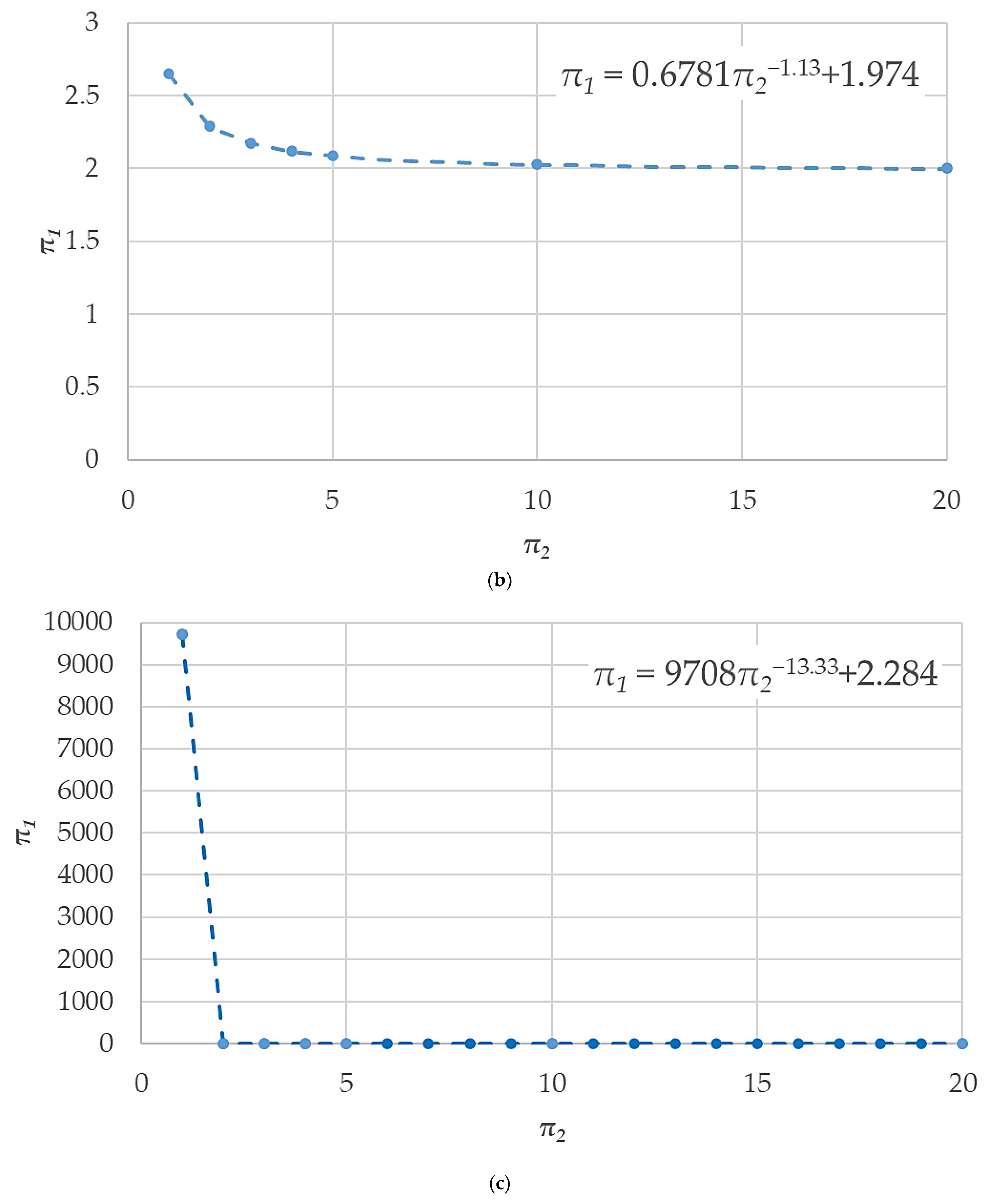
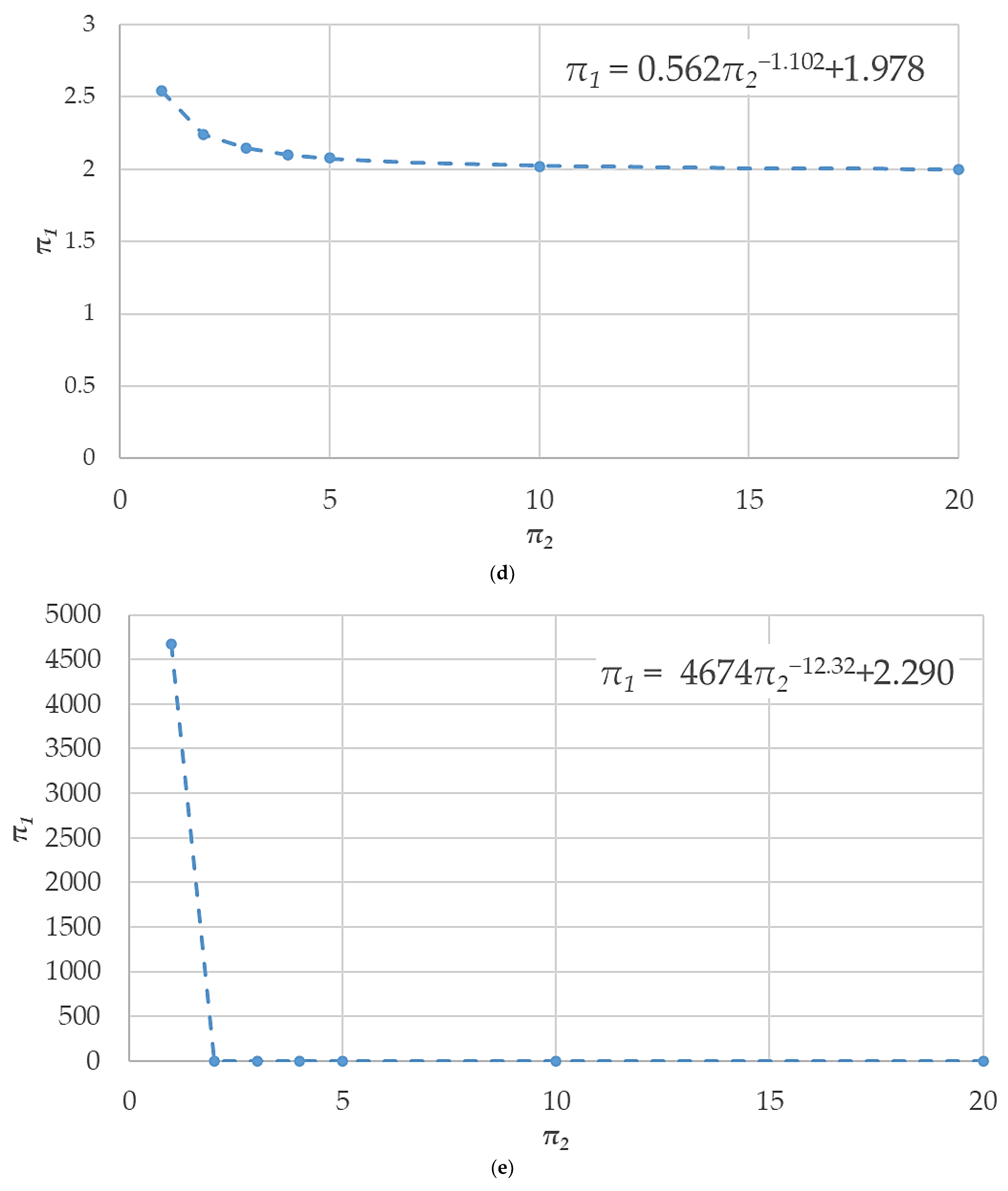
• The monomials π₂, π₃, and π₄ are calculated.
• The value of τ is determined using Equations (6)–(10). If the values of π₃ and π₄ are not those given in Equations (6)–(10), one can interpolate.
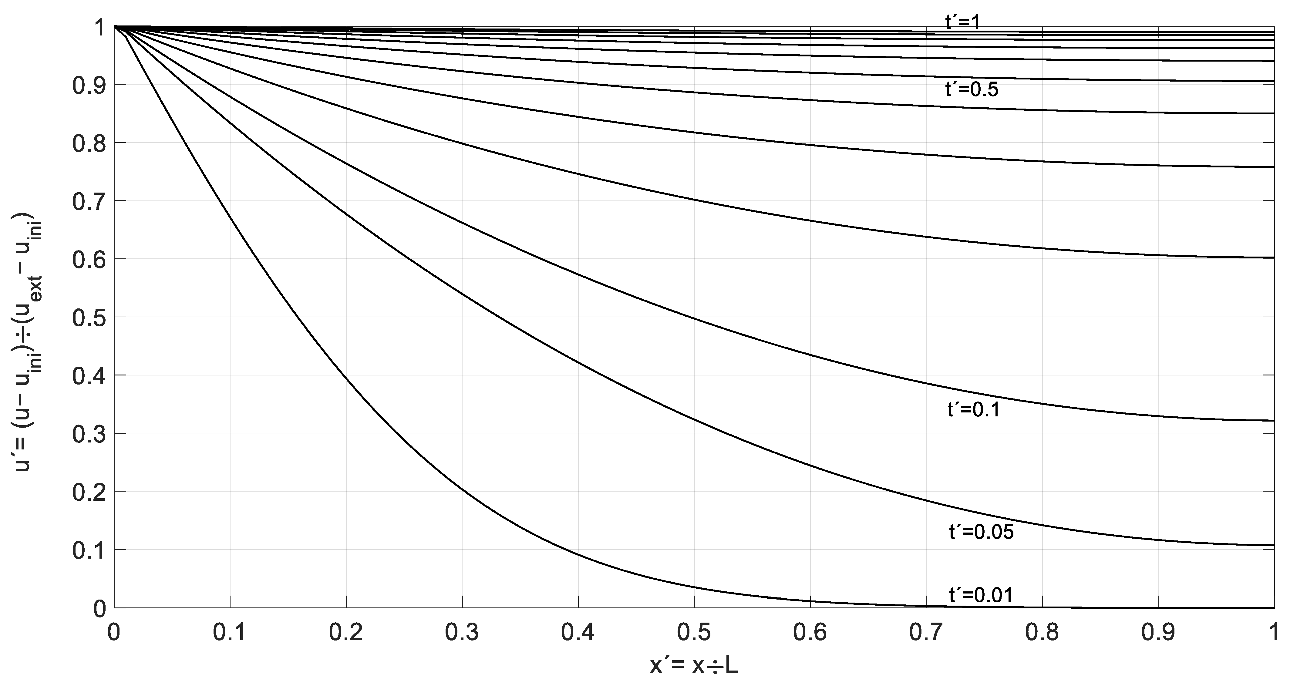
• Calculate t’ and x’ with $t^{\prime }=\frac{t}{\tau }$ and $x\prime =\frac{x}{L}$
• The value of the curve t’ is taken for position x’ in Figure 3, and the value of u is obtained from the expression given for u’, $u=u^{\prime }\left(u_{ext}-u_{ini}\right)+u_{ini}$. If the value of t’ lies between two curves, it is necessary to interpolate.

Similarly, the methodology can be used to obtain the time at which a given value of u is reached at a given position, the position at which a value of u is reached for a given time, etc.

3. Result and Validation

In the following, two types of studies are carried out to validate the methodology. In the first study, cases 1 to 3 (

Table 1. Comparison between simulated values and those calculated with the universal curve.

Case	α	β	γ	δ	ε	ζ	L (m)	uext	uini	x (m)	t (s)
1	0.5	0.5	0.5	1	0.5	6	2	2	0	0.8	0.458
2	2	1	1	2	0.25	16	1	2	0.5	0.3	0.0865
3	1	0	1	0.5	0	4	0.25	4	0	0.1	0.0145
								Universal Solution		Simulation
Case	π3	π4	π2	π1	τ	t′	x′	u		u
1	1	2	3	2.288	1.525	0.3	0.4	1.688		1.698
2	0.667	1	2	2.307	0.144	0.6	0.3	1.927		1.943
3	0	0	8	2.056	0.0321	0.45	0.4	3.673		3.667

), we analyse different cases where the parameters of the problem change, and therefore the values of the monomials change. The results obtained using the universal solution were compared with those obtained by simulation using the Network Simulation Method [32]. In case 1, it is a problem where the variable u is raised to one, since δ takes unit value. Moreover, the variable does not have initial values. In this case, all phenomena are present, that is, accumulation, drag, diffusion, and the generation and decay of species. If we compare the results obtained, following the methodology specified in the previous section, for the value of u at the 0.8 m position at a time of 0.458 s with those obtained by the simulation (Figure 4), we can see that the values obtained with both the universal solution and simulation are very similar. In the second case, where all the phenomena described above are involved again, the variable u is squared (δ = 2), affecting the phenomena of drag, generation, and the decay of species, and it also has initial values. Because these initial values influence the monomial π₃, it has a value of 0.667. Therefore, to obtain the value of τ, it is necessary to interpolate between Equations (5) and (6). Once again, the results obtained by the simulation (Figure 5) and those obtained with the universal solution have practically the same value; the difference is due to the carryover of errors in the application of the methodology. Finally, in case 3, where the phenomena of species generation and decay are not present, the variable u is raised to 0.5 (δ = 0.5) for the drag phenomena. Furthermore, the variable does not have initial values. In this case, it is necessary to interpolate between the curves of the universal solution, Figure 3, because t′ takes a value of 0.45. If we compare the results with those obtained through the simulation (Figure 6), again, they are practically the same.

In the second study, the proposed methodology was applied to a case where the boundary condition changed value (case 4). Thus, for a time between 0 and 0.0269 s, the value of u_ext is unity, and then doubles for a time between 0.0269 and 0.3212 s, as shown in

Table 2. Comparison between simulated values and those calculated with the universal curve for a case with changing boundary conditions.

Case	α	β	γ	δ		ε		ζ	L (m)	uext	t (s)	Time Range (s)
4a	1	0	1	1		0		4	1	1	0.0269	0 ≤ t ≤ 0.0269
4b	1	0	1	1		0		4	1	2	0.2943	0.0269 ≤ t ≤ 0.3212
										Universal Solution		Simulation
Case	x	uini	π3	π4	π2	π1	τ	t′	x′	u		u
4a	0.3	0	0	0	4	2.151	0.5378	0.05	0.3	0.54		0.52
	0.6	0							0.6	0.24		0.20
	0.9	0							0.9	0.11		0.07
										Universal Solution		Simulation
Case	x	uini	π3	π4	π2	π1	τ	t′	x′	u		u
4b	0.3	0.54	0	0	2	2.355	0.5888	0.5	0.3	1.92		1.91
	0.6	0.24							0.6	1.85		1.85
	0.9	0.11							0.9	1.82		1.82

. To solve this case, it must be divided into two parts, cases 4a and 4b, by applying the indicated procedure twice. For case 4a, a time of 0.0269 s was used, and there were no initial values for the study variable. Once case 4a was solved, the procedure was applied, taking as initial values for case 4b the results obtained in case 4a. On the other hand, the time used for case 4b was 0.2943 s, the difference between 0.3212 s and 0.0269 s. For both cases 4a and 4b, three positions were taken, and their results were compared with those obtained by the simulation (Figure 7). As can be seen, for case 4a there are greater differences than in case 4b with respect to the values obtained by the simulation because the methodology is more sensitive to small times due to the possible accumulated errors when applying the procedure. However, for case 4b, the results were practically the same. On the other hand, if we were in a case where the boundary condition will change more over time, we would have to apply the methodology explained in case 4 as many times as these changes occur.

Finally, the proposed methodology allows us to obtain, by means of a relatively fast procedure, the same results as those obtained by means of a numerical simulation, which means a considerable saving of time, since, in some cases, depending on the discretisation of the problem used for the simulation and the time at which the solution is to be obtained, the calculation time can be large. On the other hand, the nondimensionalisation technique can be compared with other techniques used to obtain analytical solutions of linear and nonlinear differential equations such as the differential transformation method (DTM) [36]. This method is based on obtaining the analytical solution through the Taylor series expansion. One of the main differences between both methods is that when applying the DTM, the information provided by the nondimensionalisation technique is lost, since by grouping the variables into monomials with physical meaning, it is possible to determine the importance of each of the variables or to know which phenomenon predominates over the rest.

4. Conclusions

In this paper, the nondimensionalisation technique was applied to the problem of the Burgers–Huxley equation with Dirichlet and Neumann boundary conditions to obtain a universal solution and study the behaviour of the variables of the problem.

First, after applying the nondimensionalisation technique, it can be observed that for low values of the monomial π₂, the relationship between the diffusion and drag phenomena, very high values of π₁ are needed, the relationship between the time to reach a certain value in the medium and the diffusion phenomena. Thus, in this case, as the drag phenomenon predominates over the diffusion phenomenon, it becomes difficult to reach the required value in the medium because very large time values are required. This behaviour occurs for all the studied cases of π₃ and π₄, the relationship between the drag phenomenon and the generation or decay of species, and the relationship between the generation and decay coefficients of species, respectively. On the other hand, also for all cases of π₃ and π₄, from when π₂ takes a value between two and five, π₁ tends to take a value close to two; thus, from then on, the diffusion phenomenon predominates over the rest, which are practically negligible.

Regarding the validation of the proposed procedure for a universal solution to the proposed problem, several cases have been studied by comparing the results of this procedure with those obtained through simulation, observing that they are practically the same, and the difference may be due to errors in the application of the procedure. On the other hand, the methodology has been applied to a problem where the value of the boundary changes at a certain time, observing that the results are very similar.

Finally, as a strength of the work presented, it is worth highlighting that a simple methodology is presented that allows for universal solutions to various problems in science and engineering to be obtained. As a weakness, it is highlighted that for low values of the monomial π₂ the error in the proposed equations increases, because in these cases, the monomial π₁ tends to reach infinity.

References

1. Appadu, A.R.; Tijani, Y.O. 1D Generalised Burgers-Huxley: Proposed Solutions Revisited and Numerical Solution Using FTCS and NSFD Methods. Front. Appl. Math. Stat. 2022, 7, 1–14. [Google Scholar] [CrossRef]
2. Hashim, I.; Noorani, M.S.M.; Al-Hadidi, M.R.S. Solving the generalized Burgers-Huxley equation using the Adomian decomposition method. Math Comput. Model 2006, 43, 11–12. [Google Scholar] [CrossRef]
3. Wen, Y.; Chaolu, T. Study of Burgers–Huxley Equation Using Neural Network Method. Axioms 2023, 12, 429. [Google Scholar] [CrossRef]
4. Hemel, R.; Azam, M.T.; Alam, M.S. Numerical Method for Non-Linear Conservation Laws: Inviscid Burgers Equation. J. Appl. Math. Phys. 2021, 9, 1351–1363. [Google Scholar] [CrossRef]
5. Madrid, C.; Alhama, F. Análisis Dimensional Discriminado en Mecánica de Fluidos y Transferencia de Calor; Editorial Reverté: Barcelona, Spain, 2012. [Google Scholar]
6. Cengel, Y.A.; Cimbala, J.M. Fluid Mechanics, Fundamentals and Applications, 4th ed.; McGraw-Hill Education: New York, NY, USA, 2018; Volume 91, no. 5. [Google Scholar]
7. Bejan, A. Convection Heat Transfer; Wiley-Interscience: New York, NY, USA, 1984. [Google Scholar]
8. Bejan, A.; Kraus, A.D. Heat Transfer Handbook; John Wiley & Sons: Hoboken, NJ, USA, 2003; no. 3. [Google Scholar]
9. Kreith, F.; Manglik, R.M.; Bohn, M.S. Principles of Heat Transfer, 7th ed.; Cengage Learning: Boston, MA, USA, 1999; Volume 2. [Google Scholar]
10. Heinrich, B.; Hofmann, B.; Beck, J.V.; Blackwell, B.; St. Clair, C.R., Jr. Inverse Heat Conduction. Ill-Posed Problems. New York etc., J. Wiley & Sons 1985. XVII, 308 S., £ 46.00. ISBN 0-471-08319-4. ZAMM—J. Appl. Math. Mech./Z. Angew. Math. Mech. 1987, 67, 212–213. [Google Scholar] [CrossRef]
11. Fernández, C.F.G.; Alhama, F.; Sánchez, J.F.L.; Horno, J. Application of the network method to heat conduction processes with polynomial and potential-exponentially varying thermal properties. Numeri. Heat Transf. A Appl. 1998, 33, 549–559. [Google Scholar] [CrossRef]
12. Nigri, M.R.; Pedrosa-Filho, J.J.; Gama, R.M.S. An exact solution for the heat transfer process in infinite cylindrical fins with any temperature-dependent thermal conductivity. Therm. Sci. Eng. Prog. 2022, 32, 101333. [Google Scholar] [CrossRef]
13. Albani, R.A.S.; Duda, F.P.; Pimentel, L.C.G. On the modeling of atmospheric pollutant dispersion during a diurnal cycle: A finite element study. Atmos. Environ. 2015, 118, 19–27. [Google Scholar] [CrossRef]
14. Ku, J.Y.; Rao, S.T.; Rao, K.S. Numerical simulation of air pollution in urban areas: Model development. Atmos. Environ. 1987, 21, 201–212. [Google Scholar] [CrossRef]
15. Moradpour, M.; Afshin, H.; Farhanieh, B. A numerical investigation of reactive air pollutant dispersion in urban street canyons with tree planting. Atmos. Pollut. Res. 2017, 8, 253–266. [Google Scholar] [CrossRef]
16. Fenaux, M. Modelling of Chloride Transport in Non-Saturated Concrete: From Microscale to Macroscale. Ph.D. Thesis, E.T.S.I. Caminos, Canales y Puertos (UPM), Madrid, Spain, 2013. [Google Scholar]
17. Fenaux, M.M.C.; Reyes, E.; Moragues, A.; Gálvez, J.C. Modelling of chloride transport in non-saturated concrete. From microscale to macroscale. In Proceedings of the 8th International Conference on Fracture Mechanics of Concrete and Concrete Structures, FraMCoS 2013, Toledo, Spain, 10–14 March 2013. [Google Scholar]
18. Pradelle, S.; Thiéry, M.; Baroghel-Bouny, V. Comparison of existing chloride ingress models within concretes exposed to seawater. Mater. Struct./Mater. Constr. 2016, 49, 4497–4516. [Google Scholar] [CrossRef]
19. Guimarães, A.T.C.; Climent, M.A.; De Vera, G.; Vicente, F.J.; Rodrigues, F.T.; Andrade, C. Determination of chloride diffusivity through partially saturated Portland cement concrete by a simplified procedure. Constr. Build. Mater. 2011, 25, 785–790. [Google Scholar] [CrossRef]
20. Meijers, S.J.H.; Bijen, J.M.J.M.; De Borst, R.; Fraaij, A.L.A. Computational results of a model for chloride ingress in concrete including convection, drying-wetting cycles and carbonation. Mater. Struct./Mater. Constr. 2005, 38, 145–154. [Google Scholar] [CrossRef]
21. Nielsen, E.P.; Geiker, M.R. Chloride diffusion in partially saturated cementitious material. Cem. Concr. Res. 2003, 33, 133–138. [Google Scholar] [CrossRef]
22. Martín-Pérez, B.; Pantazopoulou, S.J.; Thomas, M.D.A. Numerical solution of mass transport equations in concrete structures. Comput. Struct. 2001, 79, 1251–1264. [Google Scholar] [CrossRef]
23. Fang, X.; Wen, J.; Bonello, B.; Yin, J.; Yu, D. Wave propagation in one-dimensional nonlinear acoustic metamaterials. N. J. Phys. 2017, 19, 053007. [Google Scholar] [CrossRef]
24. Sheng, P.; Fang, X.; Wen, J.; Yu, D. Vibration properties and optimized design of a nonlinear acoustic metamaterial beam. J. Sound. Vib. 2021, 492, 115739. [Google Scholar] [CrossRef]
25. Fu, L.; Li, J.; Yang, H.; Dong, H.; Han, X. Optical solitons in birefringent fibers with the generalized coupled space–time fractional non-linear Schrödinger equations. Front. Phys. 2023, 11, 1108505. [Google Scholar] [CrossRef]
26. Yasmin, H.; Aljahdaly, N.H.; Saeed, A.M.; Shah, R. Investigating Families of Soliton Solutions for the Complex Structured Coupled Fractional Biswas–Arshed Model in Birefringent Fibers Using a Novel Analytical Technique. Fractal Fract. 2023, 7, 491. [Google Scholar] [CrossRef]
27. Rodriguez, J.N.; Omel’yanov, G. General Degasperis-Procesi equation and its solitary wave solutions. Chaos Solitons Fractals 2019, 118, 41–46. [Google Scholar] [CrossRef]
28. Zhang, K.; Alshehry, A.S.; Aljahdaly, N.H.; Shah, R.; Shah, N.A.; Ali, M.R. Efficient computational approaches for fractional-order Degasperis-Procesi and Camassa–Holm equations. Results Phys. 2023, 50, 106549. [Google Scholar] [CrossRef]
29. Sánchez-Pérez, J.F.; Alhama, I. Universal curves for the solution of chlorides penetration in reinforced concrete, water-saturated structures with bound chloride. Commun. Nonlinear Sci. Numer. Simul. 2020, 84, 105201. [Google Scholar] [CrossRef]
30. Sánchez-Pérez, J.F.; García-Ros, G.; Conesa, M.; Castro, E.; Cánovas, M. Methodology to Obtain Universal Solutions for Systems of Coupled Ordinary Differential Equations. Examples of a Continuous Flow Chemical Reactor and a Coupled Oscillator. Mathematics 2023, 11, 2303. [Google Scholar] [CrossRef]
31. Conesa, M.; Sánchez-Pérez, J.F.; García-Ros, G.; Castro, E.; Valenzuela, J. Normalization Method as a Potent Tool for Grasping Linear and Nonlinear Systems in Physics and Soil Mechanics. Mathematics 2023, 11, 4321. [Google Scholar] [CrossRef]
32. Sánchez-Pérez, J.F.; Marín-García, F.; Castro, E.; García-Ros, G.; Conesa, M.; Solano-Ramírez, J. Methodology for Solving Engineering Problems of Burgers–Huxley Coupled with Symmetric Boundary Conditions by Means of the Network Simulation Method. Symmetry 2023, 15, 1740. [Google Scholar] [CrossRef]
33. Sánchez-Pérez, J.F.; Marín, F.; Morales, J.L.; Cánovas, M.; Alhama, F. Modeling and simulation of different and representative engineering problems using network simulation method. PLoS ONE 2018, 13, e0193828. [Google Scholar] [CrossRef]
34. Sánchez-Pérez, J.F.; Mascaraque-Ramírez, C.; Nicolás, J.A.M.; Castro, E.; Cánovas, M. Study of the application of PCM to thermal insulation of UUV hulls using Network Simulation Method. Alex. Eng. J. 2021, 60, 4627–4637. [Google Scholar] [CrossRef]
35. Sánchez-Pérez, J.F.; Alhama, F.; Moreno, J.A.; Cánovas, M. Study of main parameters affecting pitting corrosion in a basic medium using the network method. Results Phys. 2019, 12, 1015–1025. [Google Scholar] [CrossRef]
36. Hussin, C.H.C.; Mandangan, A.; Kilicman, A.; Daud, M.A.; Juhan, N. Differential transformation method for solving sixth-order boundary value problems of ordinary differential equations. J. Teknol. 2016, 78, 13–19. [Google Scholar] [CrossRef]
Figure 1. Description of the study problem. Geometry, boundary, and initial conditions.
Axioms 12 01113 g001
Figure 2. Representation of π 1 versus π 2 (a) with π 3 = 0 and independent of π 4 , (b) with π 3 = 1 and π 4 = 1 , (c) with π 3 = 1 and π 4 = 2 , (d) with π 3 = 2 and π 4 = 1 , and (e) with π 3 = 2 and π 4 = 2 .
Axioms 12 01113 g002aAxioms 12 01113 g002bAxioms 12 01113 g002c
Figure 3. Universal curve for Burgers–Huxley equation with Dirichlet and symmetry (Neumann) boundary conditions.
Axioms 12 01113 g003
Figure 4. Simulation of case 1 for a time of 0.458 s.
Axioms 12 01113 g004
Figure 5. Simulation of case 2 for a time of 0.0865 s.
Axioms 12 01113 g005
Figure 6. Simulation of case 3 for a time of 0.0145 s.
Axioms 12 01113 g006
Figure 7. Simulation of case 4. (a) Case 4a: t = 0.0269 s and uext = 1, and (b) case 4b: t = 0.3212 s and uext = 2.
Axioms 12 01113 g007