
Entropy and Multi-Fractal Analysis in Complex Fractal Systems Using Graph Theory

1
Department of Mathematics and Statistics, The University of Lahore, Lahore Campus, Lahore 54600, Pakistan
2
Department of Mathematics and Statistics, College of Science, Imam Mohammad Ibn Saud Islamic University (IMSIU), Riyadh 11566, Saudi Arabia
3
Department of Mathematics, College of Science, King Saud University, Riyadh 11451, Saudi Arabia
*
Author to whom correspondence should be addressed.
†
These authors contributed equally to this work.
Axioms 2023, 12(12), 1126; https://doi.org/10.3390/axioms12121126
Submission received: 22 November 2023
/
Revised: 5 December 2023
/
Accepted: 12 December 2023
/
Published: 15 December 2023
(This article belongs to the Special Issue Advances in Graph Theory and Combinatorial Optimization)
Abstract
:In 1997, Sierpinski graphs, , were obtained by Klavzar and Milutinovic. The graph represents the complete graph and is known as the graph of the Tower of Hanoi. Through generalizing the notion of a Sierpinski graph, a graph named a generalized Sierpinski graph, denoted by , already exists in the literature. For every graph, numerous polynomials are being studied, such as chromatic polynomials, matching polynomials, independence polynomials, and the M-polynomial. For every polynomial there is an underlying geometrical object which extracts everything that is hidden in a polynomial of a common framework. Now, we describe the steps by which we complete our task. In the first step, we generate an M-polynomial for a generalized Sierpinski graph . In the second step, we extract some degree-based indices of a generalized Sierpinski graph using the M-polynomial generated in step 1. In step 3, we generate the entropy of a generalized Sierpinski graph by using the Randić index.
Keywords:
M-polynomial; Shannon’s entropy; graph entropy; Randić index; fractals; generalized Sierpinski graphsMSC:
05C07; 05C091. Introduction
M-Polynomials and Fractals
Polynomials are also connected to some other fields of science such as graph theory, networking, artificial Intelligence, machine learning, and neural networks. Polynomials related to graph theory play a vital role. In graph theory, the Hosoya polynomial is used [1] to find the distance-based topological indices. Several polynomials can be extracted from Hosoya polynomials. Cach [2] introduced the importance of Hosoya and hyper-wiener polynomials. Chou et al. [3] found the Zhang–Zhang polynomials of benzenoid chemical structures. Matching polynomials were introduced in [4,5]. Clar covered polynomials [3,6,7] and Schultz polynomials [8] have been discussed in the literature.
M-polynomials were introduced by Deutsch and Klavzar in 2015. Polynomials are very much famous in chemical graph theory and particularly in the field of mathematical chemistry. Topological indices are the sub-parts of mathematical chemistry. A topological index is the graph invariant that unveils the hidden properties of the chemical structures. Three types of topological indices are used in mathematical chemistry such as degree-based, distance-based, and spectrum-based indices. Degree-based topological indices are entirely based on the valency of the atom in the relevant chemical structure. The best property of an M-polynomial is its extraction of different degree-based topological indices from a graph. Different degree-based topological indices can be demonstrated as particular derivatives or integrals related to the M-polynomial. The benefit of M-polynomials is that, if you know the M-polynomial then you do not need to find degree-based topological indices one by one because the M-polynomial can extract multiple degree-based topological indices at once. Due to this feature of polynomials, the laborious work of finding the indices is now not necessary.
Fractals are shapes that repeat again and again in the same pattern. They occur naturally in nature. For instance, you can see the mountains, the leaves of the trees, the motion of waves, and many other shapes. There are so many shapes that are irregular in nature but fractals are not. Fractals are self-similar shapes that repeat infinitely. They simply paste copies of the same shape at different scales [9,10].
The Sierpinski graph was introduced by Klavazar and Milutinovic [11] in 1997. For further study of these graphs see reference [12]. This graph is named after the polish mathematician Waclaw Sierpinski. We denote the Sierpinski graph with , where is simply a complete graph and, after that, is called the Hanoi tower of the Sierpinski graph. This is a kind of fractal. Their introduction was first propelled by topological indices in which is isomorphic to a complete graph on the K vertices; is constructed by by adding just one edge between each copy-pair. The connectivity of the Sierpinski sieve is obtained from the Sierpinski graph of order n. The Sierpinski graph is the tower of Hanoi, while the Sierpinski gasket graphs are naturally defined by the finite number of iterations. We are motivated by the work of Klavazar and Milutinovic [11] and we have generalized the graph using this concept for degree-based topological indices and M-Polynomials.
2. Preliminaries
This definition has been taken from [11,12]. Let be a graph of order n and vertex set We denote by the set of words of size t on alphabet The letters of a word p of length t are denoted by . The concatenation of two words p and q is denoted by . We can define the t-th generalized Sierpinski graph denoted by having a vertex set and the edge set is of the form , which is an edge . Then, we have the following:
- , if ;
- and ;
- and if .
Observe that, if , then and a word w such that and . We can generate the graph as follows.
Note that and ; we make a copy n times and attach the letter r at the beginning of every label of the vertices connecting to the copy of corresponding to r. For every edge of , attach an edge between and . The vertices of this type are said to be extreme vertices of . If the graph has n extreme vertices and if the vertex r connects with edges, then the extreme vertex of also connects with edges. The numbers and are the degrees of the vertices and . These two vertices join the copies of .
The generalised Sierpinski graph has total number of vertices , in which there are three types of vertices, namely vertices of degree 2, vertices of degree 3, and vertices of degree 4, which are , and , respectively. Also, the total number of edges is .
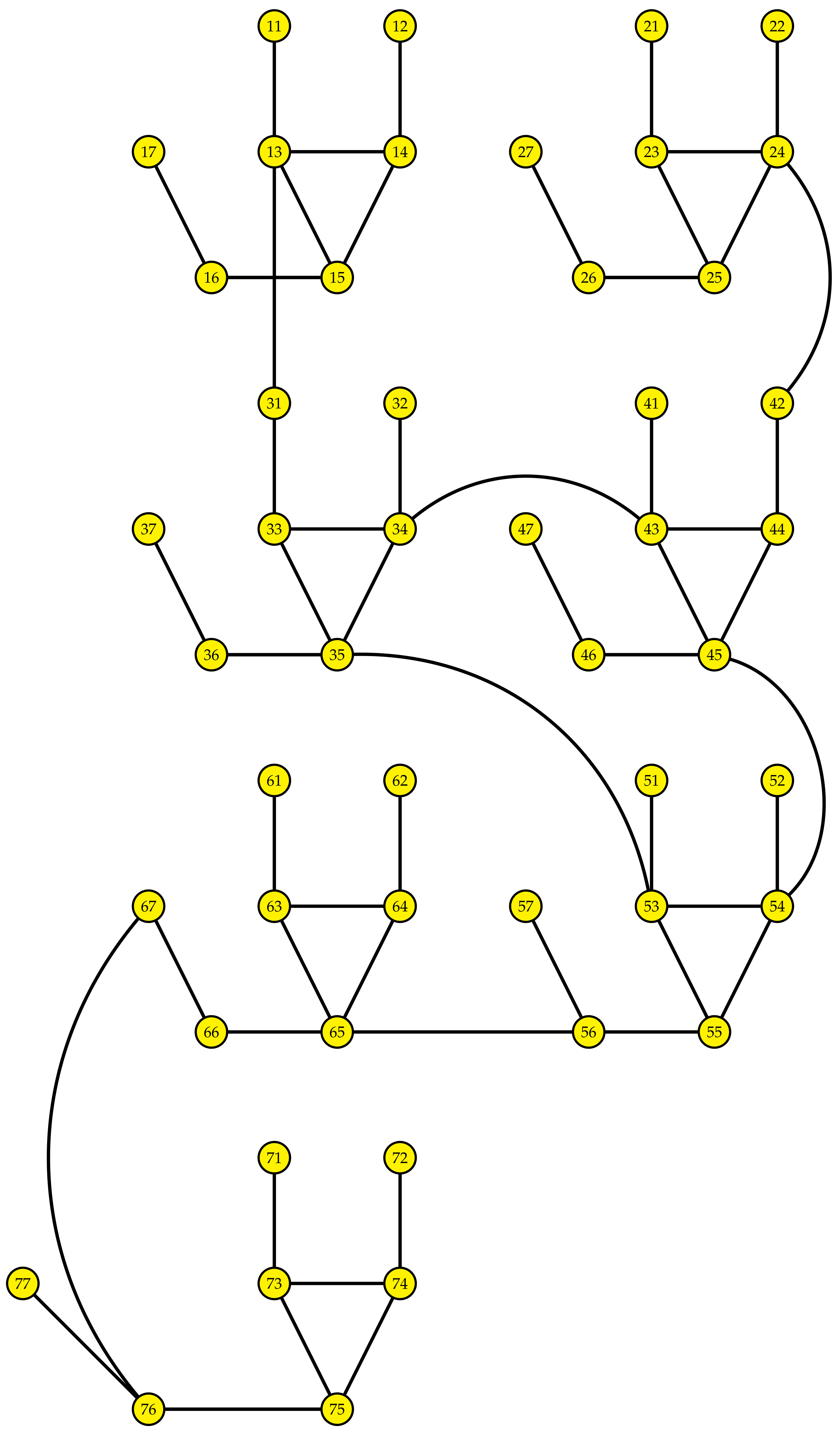
For example, for graph in Figure 1, the total number of vertices is 7 and we have given a formula for the total vertices where t is the number of iterations. If we put into this equation, . In this way, one can check for in Figure 2, and obtain an integer. Similarly, the formula for total number of edges is . If we put into this equation, . In this way, one can check for and obtain an integer.
To compute our main results, we partitioned the edges based on the degree of end vertices of each edge and represented in Table 1.
3. Results for M-Polynominal and Entropy
First, we will give some basic definitions and then will show our main results for topological indices with M-polynomials and entropy of generalized Sierpinski graphs.
Definition 1.
Let be a graph and , then let be the degree of a vertex The M-polynomial of , denoted by , is a polynomial of two variables “l” and “q”, which was introduced by Klavzar and Deutsch [13] in 2015 and is defined as
where is the number of edges of , such that
Theorem 1.
Consider the generalised Sierpinski graph , then its M-polynomial is
Proof.
Let be a generalised Sierpinski graph, then, from above, discuss the total number of vertices, , and total number of edges, . Now, the edges partition of a generalised Sierpinski graph are as follows:
,
,
,
,
,
,
,
Now apply a definition of an M-polynomial
□
Proposition 1.
Let be a generalised Sierpinski graph. Then, the topological indices are
Proof.
According to Theorem 1, we have
which is now as shown in Table 1.
First, we find and
After partial differentiation with respect to l, we have
Now, multiplying the above equation by l
Similarly, we find
Now, we have
substituting the values and in .
After substituting the values of and , we have the following result:
Similarly, in all remaining parts from 2 to 9, we have used the values of , , , to obtain our results.
Multiplying and , we obtain the following result:
First, we find and , then
Now, upon integrating, we have and
Multiplying and , we obtain the following result:
substituting the values
substituting the value in
□
Entropy, Shannon Entropy, and Graph Entropy
The measure of the unreliability of a framework is the entropy of a probability distribution; this idea was presented in Shannon’s acclaimed paper [14]. This graph entropy is applied in different fields of sciences such as chemistry, biology, nature, and human science [15,16]. There are numerous types of entropy measures, such as the graph entropy measure related to the distribution of components (vertices, edges) and probability distribution. However, the least examined graphs are entropies for weighted graphs [17].
Shannon entropy and graph entropy are two distinct concepts used in different domains of mathematics and science. Here are the key differences between the two:
Shannon entropy, often referred to as information entropy, is a concept from information theory. It quantifies the uncertainty or randomness associated with a random variable or a probability distribution. It measures the average amount of information contained in a random variable. Shannon entropy is widely used in information theory, data compression, and communication theory. It is used to analyze and measure the uncertainty or randomness in data, such as in coding theory, cryptography, and data compression algorithms.
Graph entropy is a concept used in network theory and graph theory. It quantifies the structural properties and information content of a graph (a collection of nodes and edges). It characterizes the complexity or diversity of a network’s topology. Graph entropy is applied in the analysis of complex networks, such as social networks, biological networks, and transportation networks. It is used to understand the organization and properties of these networks.
Various methods exist to compute graph entropy, depending on the aspects of the network one wants to capture. Common measures include degree entropy, clustering coefficient entropy, and betweenness centrality entropy. In summary, Shannon entropy measures the information content or randomness of data, while graph entropy quantifies the structural properties and complexity of a network or graph. They serve different purposes and are used in distinct fields of mathematics and science.
Definition 2.
Definition 3.
According to ref. [22], the Randić’ index has exhibited usefulness for assessing the degree of extension of a carbon-atom skeleton of saturated hydrocarbons.
Let be the entropy of the graph G. Now, the relationship between and is
where is a real number. Now, we will give our computations on the entropy of generalized Sierpinski graphs .
Theorem 2.
Let be a generalized Sierpinski graph. Then, the entropy of is
where α is a real number.
Proof.
The generalised Sierpinski graph is shown in Figure 2. Let denote the number of edges connecting the vertices of degree and In this graph , the total number of vertices are . The number of vertices of degree two, three, and four are , , and , respectively. The total number of edges of the generalised Sierpinski graph is . The edge partition based on the degree of the end vertices of each edge is shown in Table 2. The formula for the general Randić index is
This implies that
The formula for the entropy is given as follows:
after inserting the value of , we obtain the desired results. □
4. Conclusions
Polynomials of any order always show some applications in daily life, such as quadratic polynomials that are used to find the maximum and minimum values of the function and also to discuss the parabolic behavior of the function. In this paper, we have studied the M-Polynomial and entropy of a generalised Sierpinski graph and extracted many topological indices out of it. The advantage of an M-polynomial is the ability to obtain more than 10 degree-based topological indices at once. These results will be helpful and will open new horizons for the readers.
Author Contributions
Conceptualization, Z.S.M.; methodology, R.A.; software, Z.S.M.; validation, A.H.T. and T.A.; formal analysis, R.A.; investigation, T.A.; resources, A.H.T.; data curation, A.H.T.; writing—original draft preparation, Z.S.M.; writing—review and editing, R.A.; visualization, A.H.T.; supervision, Z.S.M.; project administration, R.A.; funding acquisition, A.H.T. All authors have read and agreed to the published version of the manuscript.
Funding
The authors extend their appreciation to the Deputyship for research & innovation, Ministry of Education in Saudi Arabia for funding this research through the project number IFP-IMSIU-2023026. The authors also appreciate the Deanship of Scientific Research at Imam Mohammad Ibn Saud Islamic University (IMSIU) for supporting and supervising this project.
Data Availability Statement
Data are contained within the article.
Conflicts of Interest
The authors declare no conflict of interest.
References
- Gutman, I.; Dehmer, M.; Zhang, Y.; Ilic, A. Altenburg, Wiener, and Hosoya polynomials. In Distance in Molecular Graphs Theory; University of Kragujevac Rectorate: Kragujevac, Serbia, 2012; pp. 49–70. [Google Scholar]
- Cash, G.G. Relationship between the Hosoya polynomial and the hyper-Wiener index. Appl. Math. Lett. 2002, 15, 893–895. [Google Scholar] [CrossRef]
- Chou, C.-P.; Witek, H.A. Closed-form formulas for the Zhang-Zhang polynomials of benzenoid structures: Chevrons and generalized chevrons. MATCH Commun. Math. Comput. Chem. 2014, 72, 105–124. [Google Scholar]
- Farrell, E.J. An introduction to matching polynomials. J. Combin. Theory Ser. B 1979, 27, 75–86. [Google Scholar] [CrossRef]
- Gutman, I. Degree-based topological indices. Croat. Chem. Acta 2013, 86, 351–361. [Google Scholar] [CrossRef]
- Zhang, H.; Shiu, W.C.; Sun, P.-K. A relation between Clar covering polynomial and cube polynomial. MATCH Commun. Math. Comput. Chem. 2013, 70, 477–492. [Google Scholar]
- Zhang, H.; Zhang, F. The Clar covering polynomial of hexagonal systems I. Discrete Appl. Math. 1996, 69, 147–167. [Google Scholar] [CrossRef]
- Hassani, F.; Iranmanesh, A.; Mirzaie:, S. Schultz and modified Schultz polynomials of C100 fullerene. MATCH Commun. Math. Comput. Chem. 2013, 69, 87–92. [Google Scholar]
- Alonso-Ruiz, P.; Kelleher, D.J.; Teplyaev, A. Energy and Laplacian on Hanoi-type fractal quantum graphs. J. Phys. Math. Theor. 2016, 49, 165206. [Google Scholar] [CrossRef]
- Mograby, G.; Derevyagin, M.; Dunne, G.V.; Teplyaev, A. Spectra of perfect state transfer Hamiltonians on fractal-like graphs. J. Phys. Math. Theor. 2021, 54, 125301. [Google Scholar] [CrossRef]
- Klavzar, S.; Milutinovic, U. Graphs S(n,k) and a variant of the Tower of Hanoi problem. Czechoslov. Math. J. 1997, 47, 95104. [Google Scholar] [CrossRef]
- Gravier, S.; Kovse, M.; Parreau, A. Generalized Sierpinski graphs. In Proceedings of the Euro-Comb11, Budapest, Hungary, 29 August–2 September 2011. [Google Scholar]
- Deutsch, E.; Klavžar, S. M-polynomial and degree-based topological indices. Iran. J. Math. Chem. 2015, 6, 93–102. [Google Scholar]
- Shannon, C.; Weaver, W. The Mathematical Theory of Communication; University of Illinois Press: Urbana, IL, USA, 1949. [Google Scholar]
- Dehmer, M.; Mowshowitz, A. A history of graph entropy measures. Inf. Sci. 2011, 181, 57–78. [Google Scholar] [CrossRef]
- Mowshowitz, A.; Dehmer, M. Entropy and the complexity of graphs revisited. Entropy 2012, 14, 559–570. [Google Scholar] [CrossRef]
- Chen, Z.; Dehmer, M.; Emmert-Streib, F.; Shi, Y. Entropy of weighted graphs with Randić weights. Entropy 2015, 17, 3710–3723. [Google Scholar] [CrossRef]
- Eagle, N.; Macy, M.; Claxton, R. Network diversity and economic development. Science 2010, 328, 1029–1031. [Google Scholar] [CrossRef] [PubMed]
- Li, X.; Gutman, I. Mathematical Aspects of Randic-Type Molecular Structure Descriptors; University of Kragujevac and Faculty of Science Kragujevac: Kragujevac, Serbia, 2006. [Google Scholar]
- Li, X.; Shi, Y.; Xu, T. Unicyclic graphs with maximum general Randic index for α>0. MATCH Commun. Math. Comput. Chem. 2006, 56, 557–570. [Google Scholar]
- Li, X.; Shi, Y.; Zhong, L. Minimum general Randic index on chemical trees with given order and number of pendent vertices. MATCH Commun. Math. Comput. Chem. 2008, 60, 539–554. [Google Scholar]
- Randic, M. On characterization of molecular branching. J. Am. Chem. Soc. 1975, 97, 6609–6615. [Google Scholar] [CrossRef]
Figure 1.
Seed graph .
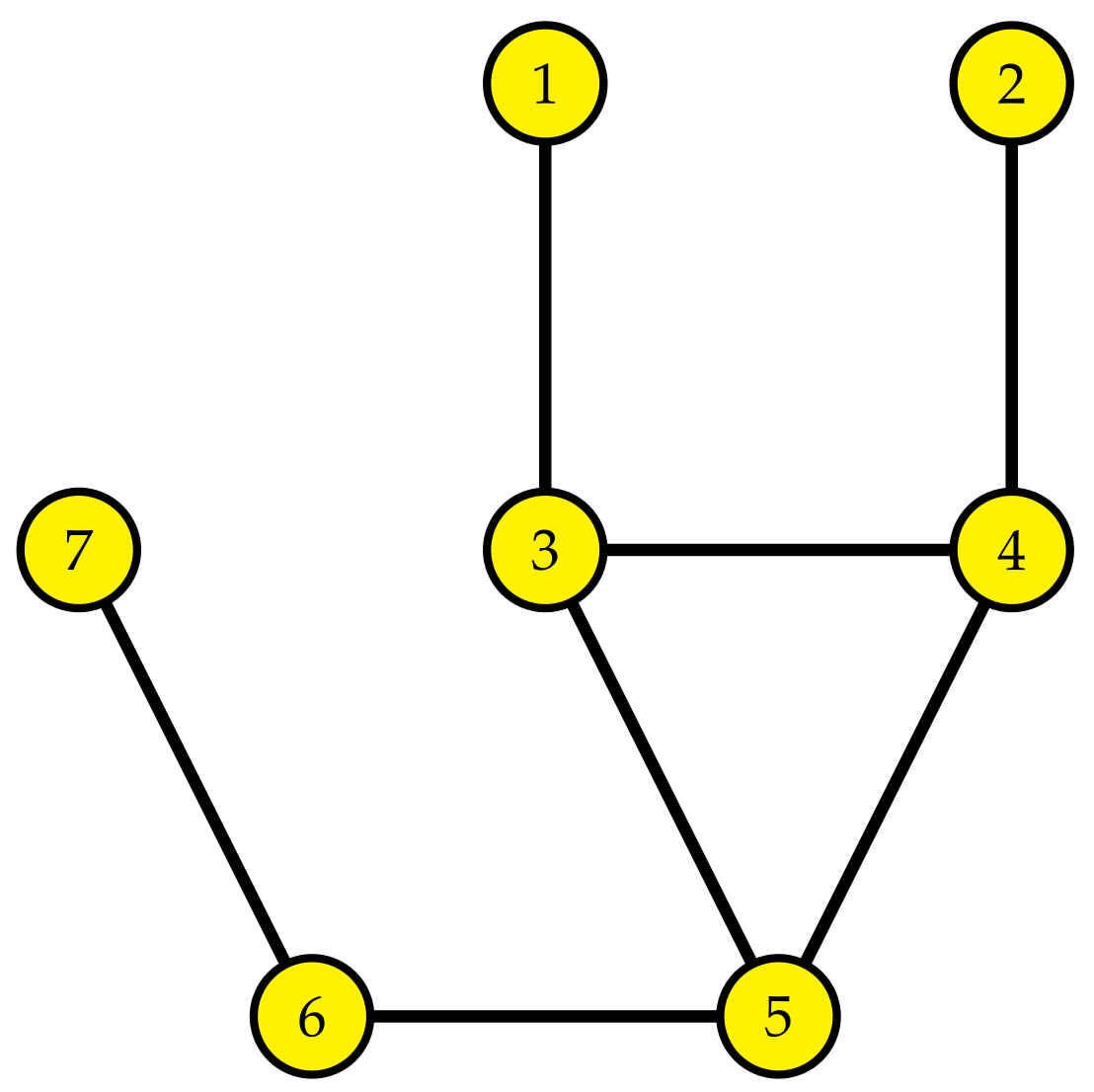
Figure 2.
Generalised Sierpinski graph generated from its seed graph .

Table 1.
The edge partition of graph based on the degree of end vertices of each edge.
| (d,d), where, pj∈ E(G) | E | Number of Edges |
|---|---|---|
| (1, 2) | E | |
| (1, 3) | E | |
| (1, 4) | E | |
| (2, 2) | E | |
| (2, 3) | E | |
| (2, 4) | E | |
| (3, 3) | E | |
| (3, 4) | E | |
| (4, 4) | E |
Table 2.
M-polynomial topological indices.
| Topological Indices | Derivation from M(Sie(,t),l,q) |
|---|---|
| First Zagreb index | |
| Second Zagreb index | |
| Second modified Zagreb index | |
| General Randić index, | |
| Inverse general Randić index, | |
| Symmetric division index | |
| Harmonic index | |
| Inverse sum index | |
| Augmented Zagreb |
where
Disclaimer/Publisher’s Note: The statements, opinions and data contained in all publications are solely those of the individual author(s) and contributor(s) and not of MDPI and/or the editor(s). MDPI and/or the editor(s) disclaim responsibility for any injury to people or property resulting from any ideas, methods, instructions or products referred to in the content. |
© 2023 by the authors. Licensee MDPI, Basel, Switzerland. This article is an open access article distributed under the terms and conditions of the Creative Commons Attribution (CC BY) license (https://creativecommons.org/licenses/by/4.0/).
Share and Cite
MDPI and ACS Style
Mufti, Z.S.; Tedjani, A.H.; Anjum, R.; Alsuraiheed, T. Entropy and Multi-Fractal Analysis in Complex Fractal Systems Using Graph Theory. Axioms 2023, 12, 1126. https://doi.org/10.3390/axioms12121126
AMA Style
Mufti ZS, Tedjani AH, Anjum R, Alsuraiheed T. Entropy and Multi-Fractal Analysis in Complex Fractal Systems Using Graph Theory. Axioms. 2023; 12(12):1126. https://doi.org/10.3390/axioms12121126
Chicago/Turabian StyleMufti, Zeeshan Saleem, Ali H. Tedjani, Rukhshanda Anjum, and Turki Alsuraiheed. 2023. "Entropy and Multi-Fractal Analysis in Complex Fractal Systems Using Graph Theory" Axioms 12, no. 12: 1126. https://doi.org/10.3390/axioms12121126
Note that from the first issue of 2016, this journal uses article numbers instead of page numbers. See further details here.