Abstract
This paper outlines a study into the exact solutions of the (2+1)-dimensional Heisenberg ferromagnetic spin chain equation that is used to illustrate the ferromagnetic materials of magnetic ordering by applying two recent techniques, namely, the Sardar-subequation method and extended rational sine–cosine and sinh–cosh methods. Abundant exact solutions such as the bright soliton, dark soliton, combined bright–dark soliton, singular soliton and other periodic wave solutions expressed by the generalized trigonometric, generalized hyperbolic, trigonometric and hyperbolic functions are obtained. The numerical results are illustrated in the form of 3D plots, 2D contours and 2D curves by choosing proper parametric values to interpret the physical behavior of the model. The obtained results in this work are expected to provide a rich platform for constructing the soliton solutions of PDEs in physics.
1. Introduction
In recent decades, scholars have proposed many important nonlinear evolution equations to simulate different nonlinear phenomena involved in optics [1,2,3,4,5], plasma physics [6,7], thermodynamics [8], vibration [9,10], quantum mechanics [11,12] and so on. The question of how to obtain the exact solutions of nonlinear partial differential equations has been a hot topic for mathematicians and physicists. So far, many effective and powerful methods have been put forward such as the extended trial equation method [13,14], sine–Gordon expansion method [15,16], generalized (G’/G) expansion method [17,18], extended rational sine–cosine and sinh–cosh method [19,20], Wang’s Bäcklund transformation-based method [21], the extended FAN subequation method [22] and so on [23,24,25,26,27,28,29]. In this paper, we aim to study the (2+1)-dimensional Heisenberg ferromagnetic spin chain equation (HFSCE) controlled by a new integrable (2+1)-dimensional nonlinear Schrödinger-type equation which reads as [30,31]:
where is the complex function of x, y, t, , , , . The descriptions of these parameters are shown in Table 1. Equation (1) is usually used to describe the wave propagation in the Heisenberg ferromagnetic spin chain. In [30], two methods are used to seek for diverse solitons, namely the generalized Riccati mapping method and improved auxiliary equation. In [31], the Jacobi elliptic expansion method is adopted and bright and dark soliton solutions are obtained. In [32], the theory of dynamical systems is introduced for the construction of the bounded traveling wave solutions. In [33], the modified Khater method is used to deal with Equation (1). The generalized tanh method is employed to solve Equation (1) in [34], and dark, dark–bright or combined optical and singular soliton solutions are attained. In [35], the authors use two approaches, namely the modified F-Expansion and projective Riccati equation methods, to investigate Equation (1). In [36], the extended FAN subequation method is presented to study Equation (1) and different soliton solutions like the bright, dark, combined bright–dark and other wave solutions are constructed. In our work [37], the variational method and subequation method are used to deal with Equation (1) and different soliton solutions are constructed. As the expansion of our previous achievements, in this study we will seek to obtain the exact solutions of Equation (1) by other new methods, namely the Sardar-subequation method (SSBM) and extended rational sine–cosine and sinh–cosh methods (ERSSM). The structure of this paper is as follows. We provide a detailed introduction of the algorithms of the two methods in Section 2. We apply the two methods to find the exact solutions in Section 3. In Section 4, the behaviors of some solutions and their physical interpretations are given. Finally, we reach a conclusion in Section 5.

Table 1.
The descriptions of the coefficients.
2. The Methods
The purpose of this section is to provide a brief introduction to the SSBM and ERSSM.
Consider a general PDE as:
Making use of the transformation as:
where m, n are the wave numbers, k is the group velocity of the wave.
It can turn Equation (2) into an ODE which reads as:
2.1. The SSBM
Based on the SSBM [38,39,40], we can suppose Equation (4) has the solution as:
where are the constants to be determined later. There is:
where , , are constants. Equation (6) has the following solutions for different conditions:
Case I: When and , we have:
where , .
Case II: When and , we have:
where , .
Case III: When and , we have:
where , .
Case IV: When and , we have:
where , .
2.2. The ERSSM
(1) The extended rational sine–cosine method
Supposing the solution of Equation (4) is [19]:
Or
where , and are unknown constants to be determined.
Taking Equation (7) or Equation (8) into Equation (4), making the corresponding adjustments and setting the coefficients of or as zero yields a system of algebraic equations. Solving it, the unknown coefficients can be obtained.
(2) The extended rational sinh–cosh method
The solution of Equation (4) is considered as [41]:
Or
By the same means, we obtain a system of algebraic equations by equating the coefficients of or to zero in this case. Solving the system, we can determine the unknown coefficients.
3. Applications
The following complex transformation is introduced:
Taking Equation (11) into Equation (1) produces the following the imaginary and real parts, respectively as:
where . We re-write Equation (13) as:
where
3.1. Application of the Sardar-Subequation Method
The solution of Equation (14) is assumed as:
A balance between and gives , so Equation (16) reduces to:
Inserting Equation (17) with Equation (6) into Equation (14) and adjusting the obtained results yields:
Solving them, we obtain:
Taking Equation (15) into it has:
So, the solutions of Equation (1) are:
Case I: If and , we have:
which is the bright soliton solution for and .
which represents the singular soliton solution for and .
Case II: If and , the singular periodic wave solutions is as:
and
which are both under the conditions for and .
Case III: If and , Equation (1) formats the singular periodic wave solutions as:
which are all under the conditions for and .
Case IV: When and , Equation (1) has the following different soliton solutions under the conditions for and :
where Equation (28) is the dark soliton solution, Equations (29)–(32) represent the singular soliton solution, and Equation (30) means the dark–bright soliton solution.
3.2. Application of the Extended Rational Sine–Cosine and Sinh–Cosh Methods
Supposing the solution of Equation (14) as
Plugging it into Equation (14) and taking the proper treatments gives:
: ,
: ,
: ,
Solving them, we obtain:
Case I: , , ,
In the view of Equation (15), we have the singular periodic wave solutions of Equation (1) as:
Case II: , , ,
In the view of Equation (15), Equation (1) has the singular periodic wave solutions as:
Assume Equation (14) has the solution as:
Similarly, we have:
: ,
: ,
: ,
Solving above equations gives:
Case I: , , ,
In the view of Equation (15), we have the singular periodic wave solutions of Equation (1) as:
Case II: , , ,
In the view of Equation (15), we have the singular periodic wave solutions as:
We can also assume the solution of Equation (14) as:
Putting it into Equation (14) yields:
: ,
: ,
: ,
Solving them produces:
Case I: , , ,
In the view of Equation (15), we obtain the following soliton solutions of Equation (1) as:
which means that the dark soliton solution for and .
which is the singular soliton solution for and .
Case II: , , ,
In the light of Equation (15), we obtain the dark soliton solution for Equation (1) as:
which is under the condition for and .
We can also assume the solution of Equation (14) as:
In the same manner, we have:
: ,
: ,
: ,
Solving them produces:
Case I: , , ,
In the view of Equation (15), we have the singular soliton solutions for Equation (1) as:
which are all under the conditions for and .
Case II: , , ,
In the light of Equation (15), we have the singular soliton solutions for Equation (1) as:
which are both under the conditions for and .
By comparing the solutions of Equations (46) and (47) obtained by the ERSSM with the solutions of Equations (28) and (29) for and , which were attained by the SSBE, respectively, good agreement is reached, which reveals that the proposed methods are correct and effective. In addition, a comparison between the obtained results and our previous works [39] reveals that Equations (28) and (46) (for and ) are the same as the solution Equation (46) obtained in [37] for , . Equations (29) and (47) (for and ) are the same as the solution Equation (47) reported in [37] for , .
4. Discussion and the Physical Interpretations
The purpose of this section is to present the behaviors of the soliton solutions graphically with the help of the Mathematica software.
We illustrate the behaviors of , , , and via the 3D plot, 2D contour and 2D curve to understand the physical behavior of the model by choosing the proper parameters in Figure 1, Figure 2, Figure 3, Figure 4 and Figure 5. We can find that the wave form of is the bright soliton, the wave form of is the singular soliton, the profiles of the and are both the dark solitons and the profile of is the combined dark–bright soliton.
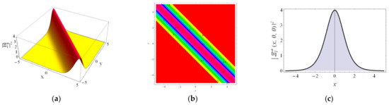
Figure 1.
The profile of the bright soliton solution with the parameters , , , , , , , , , (a) the 3D contour for . (b) the 2D contour, (c) the 2D curve for , .
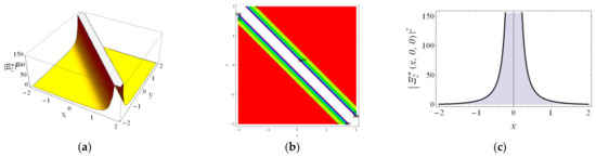
Figure 2.
The profile of the singular soliton solution with the parameters , , , , , , , , , (a) the 3D contour for . (b) the 2D contour, (c) the 2D curve for , .
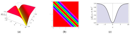
Figure 3.
The profile of the dark soliton solution with the parameters , , , , , , , , , (a) the 3D contour for . (b) the 2D contour, (c) the 2D curve for , .
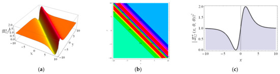
Figure 4.
The profile of the combined dark-bright soliton solution with the parameters , , , , , , , , , (a) the 3D contour for . (b) the 2D contour, (c) the 2D curve for , .
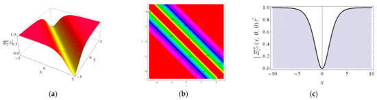
Figure 5.
The profile of the dark soliton solution with the parameters , , , , , , , , , (a) the 3D contour for . (b) the 2D contour, (c) the 2D curve for , .
5. Conclusions
Two effective approaches, namely the Sardar-subequation method and extended rational sine–cosine and sinh–cosh methods, have been used in this work to search for the exact solutions of the (2+1)-dimensional HFSCE. Various soliton solutions, such as the bright soliton, dark soliton, combined dark–bright soliton, singular soliton and other periodic wave solutions are constructed and expressed in the form of generalized trigonometric, generalized hyperbolic, trigonometric and hyperbolic functions. Numerical simulation of the different soliton solutions is presented via the 3D plots, 2D contours and 2D curves to interpret the physical behavior of the model by assigning appropriate parameters. The comparison between the solutions obtained by the SSBE and those obtained by the ERSSM shows that the solutions Equations (46) and (47) are the same as those for Equations (28) and (29), respectively for and , which strongly proves the correctness and effectiveness of the proposed methods.
Recently, the fractal and fractional calculus [42,43,44,45,46] has received public attention in many fields. The methods proposed in this work can be employed to study the soliton and travelling wave solutions of the fractal and fractional PDEs arising in the field of physics.
Author Contributions
Conceptualization, K.-J.W.; methodology, K.-J.W.; writing—original draft preparation, K.-J.W.; supervision, K.-J.W.; writing—review and editing, F.S.; data curation, F.S. All authors have read and agreed to the published version of the manuscript.
Funding
This work is supported by the Key Programs of Universities in Henan Province of China (22A140006), Program of Henan Polytechnic University (B2018-40), the Innovative Scientists and Technicians Team of Henan Provincial High Education (21IRTSTHN016), the doctoral Fund Project of Henan Polytechnic University (B2017-56).
Data Availability Statement
The data that support the findings of this study are available from the corresponding author upon reasonable request.
Conflicts of Interest
This work does not have any conflict of interest.
References
- Lü, X.; Chen, S.-J. New general interaction solutions to the KPI equation via an optional decoupling condition approach. Commun. Nonlinear Sci. Numer. Simul. 2021, 103, 105939. [Google Scholar] [CrossRef]
- Alam, M.N.; Tunç, C. Constructions of the optical solitons and other solitons to the conformable fractional Zakharov-Kuznetsov equation with power law nonlinearity. J. Taibah Univ. Sci. 2020, 14, 94–100. [Google Scholar] [CrossRef]
- Hosseini, K.; Mirzazadeh, M.; Rabiei, F.; Baskonus, H.M.; Yel, G. Dark optical solitons to the Biswas-Arshed equation with high order dispersions and absence of the self-phase modulation. Optik 2020, 209, 164576. [Google Scholar] [CrossRef]
- Hosseini, K.; Salahshour, S.; Mirzazadeh, M. Bright and dark solitons of a weakly nonlocal Schrödinger equation involving the parabolic law nonlinearity. Optik 2021, 227, 166042. [Google Scholar] [CrossRef]
- Wang, K.J. Diverse wave structures to the modified Benjamin-Bona-Mahony equation in the optical illusions field. Mod. Phys. Lett. B 2023, 2023, 2350012. [Google Scholar] [CrossRef]
- Ali, K.K.; Yilmazer, R.; Baskonus, H.M.; Bulut, H. New wave behaviors and stability analysis of the Gilson–Pickering equation in plasma physics. Indian J. Phys. 2021, 95, 1003–1008. [Google Scholar] [CrossRef]
- Cheemaa, N.; Seadawy, A.R.; Chen, S. Some new families of solitary wave solutions of the generalized Schamel equation and their applications in plasma physics. Eur. Phys. J. Plus 2019, 134, 117. [Google Scholar] [CrossRef]
- Sohail, M.; Chu, Y.M.; El-zahar, E.R.; Nazir, U.; Naseem, T. Contribution of joule heating and viscous dissipation on three dimensional flow of Casson model comprising temperature dependent conductance utilizing shooting method. Phys. Scr. 2021, 96, 085208. [Google Scholar] [CrossRef]
- He, J.H.; Yang, Q.; He, C.H.; Khan, Y. A simple frequency formulation for the tangent oscillator. Axioms 2021, 10, 320. [Google Scholar] [CrossRef]
- Wang, K.; Si, J. Dynamic properties of the attachment oscillator arising in the nanophysics. Open Phys. 2023, 21, 20220214. [Google Scholar] [CrossRef]
- Taiwo, T.J.; Njah, A.N.; Oghre, E.O. Solution of Schrodinger equation using Tridiagonal representation approach in nonrelativistic quantum mechanics: A pedagogical approach. arXiv 2018, arXiv:1810.05509. [Google Scholar]
- Van Assche, W. Solution of an open problem about two families of orthogonal polynomials. SIGMA. Symmetry Integr. Geom. Methods Appl. 2019, 15, 005. [Google Scholar]
- Gurefe, Y.; Misirli, E.; Sonmezoglu, A.; Ekici, M. Extended trial equation method to generalized nonlinear partial differential equations. Appl. Math. Comput. 2013, 219, 5253–5260. [Google Scholar] [CrossRef]
- Hu, J.Y.; Feng, X.B.; Yang, Y.F. Optical envelope patterns perturbation with full nonlinearity for Gerdjikov–Ivanov equation by trial equation method. Optik 2021, 240, 166877. [Google Scholar] [CrossRef]
- Baskonus, H.M.; Bulut, H.; Sulaiman, T.A. New complex hyperbolic structures to the lonngren-wave equation by using sine-gordon expansion method. Appl. Math. Nonlinear Sci. 2019, 4, 129–138. [Google Scholar] [CrossRef]
- Yel, G.; Baskonus, H.M.; Bulut, H. Novel archetypes of new coupled Konno-Oono equation by using sine-Gordon expansion method. Opt. Quantum Electron. 2017, 49, 285. [Google Scholar] [CrossRef]
- Alam, M.N.; Akbar, M.A. Exact traveling wave solutions of the KP-BBM equation by using the new approach of generalized (G′/G)-expansion method. SpringerPlus 2013, 2, 617. [Google Scholar] [CrossRef]
- Teymuri Sindi, C.; Manafian, J. Wave solutions for variants of the KdV-Burger and the K (n, n)-Burger equations by the generalized G′/G-expansion method. Math. Methods Appl. Sci. 2017, 40, 4350–4363. [Google Scholar] [CrossRef]
- Mahak, N.; Akram, G. Exact solitary wave solutions by extended rational sine-cosine and extended rational sinh-cosh techniques. Phys. Scr. 2019, 94, 115212. [Google Scholar] [CrossRef]
- Mahak, N.; Akram, G. Extension of rational sine-cosine and rational sinh-cosh techniques to extract solutions for the perturbed NLSE with Kerr law nonlinearity. Eur. Phys. J. Plus 2019, 134, 159. [Google Scholar] [CrossRef]
- Wang, K.J.; Liu, J.H. Diverse optical solitons to the nonlinear Schrödinger equation via two novel techniques. Eur. Phys. J. Plus 2023, 138, 74. [Google Scholar] [CrossRef]
- El-Wakil, S.A.; Abdou, M.A. The extended Fan sub-equation method and its applications for a class of nonlinear evolution equations. Chaos Solitons Fractals 2008, 36, 343–353. [Google Scholar] [CrossRef]
- Liu, J.-G.; Ye, Q. Stripe solitons and lump solutions for a generalized Kadomtsev-Petviashvili equation with variable coefficients in fluid mechanics. Nonlinear Dyn 2019, 96, 23–29. [Google Scholar] [CrossRef]
- Darwish, A.; Ahmed, H.M.; Arnous, A.H.; Shehab, M.F. Optical solitons of Biswas–Arshed equation in birefringent fibers using improved modified extended tanh-function method. Optik 2021, 227, 165385. [Google Scholar] [CrossRef]
- Liu, J.-G.; Wazwaz, A.M.; Zhu, W.H. Solitary and lump waves interaction in variable-coefficient nonlinear evolution equation by a modified Ansatz with variable coefficients. J. Appl. Anal. Comput. 2022, 12, 517–532. [Google Scholar] [CrossRef]
- Wang, K.J.; Liu, J.H.; Si, J.; Shi, F.; Wang, G.-D. N-soliton, breather, lump solutions and diverse travelling wave solutions of the fractional (2+1)-dimensional Boussinesq equation. Fractals 2023, 31, 2350023. [Google Scholar] [CrossRef]
- Zulfiqar, A.; Ahmad, J. Soliton solutions of fractional modified unstable Schrödinger equation using Exp-function method. Results Phys. 2020, 19, 103476. [Google Scholar] [CrossRef]
- Barman, H.K.; Roy, R.; Mahmud, F.; Akbar, M.A.; Osman, M.S. Harmonizing wave solutions to the Fokas-Lenells model through the generalized Kudryashov method. Optik 2021, 229, 166294. [Google Scholar] [CrossRef]
- Ji-Guang, R.; Li-Hong, W.; Yu, Z.; He, J. Rational solutions for the Fokas system. Commun. Theor. Phys. 2015, 64, 605. [Google Scholar]
- Seadawy, A.R.; Nasreen, N.; Lu, D.; Arshad, M. Arising wave propagation in nonlinear media for the (2+1)-dimensional Heisenberg ferromagnetic spin chain dynamical model. Phys. A Stat. Mech. Its Appl. 2020, 538, 122846. [Google Scholar] [CrossRef]
- Hosseini, K.; Salahshour, S.; Mirzazadeh, M.; Ahmadian, A.; Baleanu, D.; Khoshrang, A. The (2+1)-dimensional Heisenberg ferromagnetic spin chain equation: Its solitons and Jacobi elliptic function solutions. Eur. Phys. J. Plus 2021, 136, 1–9. [Google Scholar] [CrossRef]
- Yang, D. Traveling waves and bifurcations for the (2+1)-dimensional Heisenberg ferromagnetic spin chain equation. Optik 2021, 248, 168058. [Google Scholar] [CrossRef]
- Sahoo, S.; Tripathy, A. New exact solitary solutions of the (2+1)-dimensional Heisenberg ferromagnetic spin chain equation. Eur. Phys. J. Plus 2022, 137, 390. [Google Scholar] [CrossRef]
- Inc, M.; Aliyu, A.I.; Yusuf, A.; Baleanu, D. Optical solitons and modulation instability analysis of an integrable model of (2+1)-dimensional Heisenberg ferromagnetic spin chain equation. Superlattices Microstruct. 2017, 112, 628–638. [Google Scholar] [CrossRef]
- Aliyu, A.I.; Li, Y.; İnç, M.; Wang, G. Solitons and complexitons to the (2+1)-dimensional Heisenberg ferromagnetic spin chain model. Int. J. Mod. Phys. B 2019, 33, 1950368. [Google Scholar] [CrossRef]
- Osman, M.S.; Tariq, K.U.; Bekir, A.; Elmoasry, A. Investigation of soliton solutions with different wave structures to the (2+1)-dimensional Heisenberg ferromagnetic spin chain equation. Commun. Theor. Phys. 2020, 72, 035002. [Google Scholar] [CrossRef]
- Wang, K.-J.; Shi, F.; Wang, G.-D. Abundant soliton structures to the (2+1)-dimensional Heisenberg ferromagnetic spin chain dynamical model. Adv. Math. Phys. 2023, 2023, 4348758. [Google Scholar] [CrossRef]
- Rehman, H.U.; Seadawy, A.R.; Younis, M.; Yasin, S.; Raza, S.T.R.; Althobaiti, S. Monochromatic optical beam propagation of paraxial dynamical model in Kerr media. Results Phys. 2021, 31, 105015. [Google Scholar] [CrossRef]
- Wang, K.J.; Si, J. Diverse optical solitons to the complex Ginzburg-Landau equation with Kerr law nonlinearity in the nonlinear optical fiber. Eur. Phys. J. Plus 2023, 138, 187. [Google Scholar] [CrossRef]
- Esen, H.; Ozdemir, N.; Secer, A.; Bayram, M. On solitary wave solutions for the perturbed Chen-Lee-Liu equation via an analytical approach. Optik 2021, 245, 167641. [Google Scholar] [CrossRef]
- Cinar, M.; Onder, I.; Secer, A.; Yusuf, A.; Sulaiman, T.A.; Bayram, M.; Aydin, H. The analytical solutions of Zoomeron equation via extended rational sin-cos and sinh-cosh methods. Phys. Scr. 2021, 96, 094002. [Google Scholar] [CrossRef]
- Wang, K.-J.; Shi, F.; Si, J.; Liu, J.-H.; Wang, G.-D. Non-differentiable exact solutions of the local fractional Zakharov-Kuznetsov equation on the Cantor sets. Fractals 2023, 31, 2350028. [Google Scholar] [CrossRef]
- Seadawy, A.R.; Bilal, M.; Younis, M.; Rizvi, S.T.R. Resonant optical solitons with conformable time-fractional nonlinear Schrödinger equation. Int. J. Mod. Phys. B 2021, 35, 2150044. [Google Scholar] [CrossRef]
- Wang, K.L. Novel scheme for the fractal-fractional short water wave model with unsmooth boundaries. Fractals 2022, 30, 2250193. [Google Scholar] [CrossRef]
- Wang, K.L. Novel travelling wave solutions for the fractal Zakharov-Kuznetsov-Benjamin-Bona-Mahony model. Fractals 2022, 30, 2250170. [Google Scholar] [CrossRef]
- Zhang, S.; Zhang, H.Q. Fractional sub-equation method and its applications to nonlinear fractional PDEs. Phys. Lett. A 2011, 375, 1069–1073. [Google Scholar] [CrossRef]


Disclaimer/Publisher’s Note: The statements, opinions and data contained in all publications are solely those of the individual author(s) and contributor(s) and not of MDPI and/or the editor(s). MDPI and/or the editor(s) disclaim responsibility for any injury to people or property resulting from any ideas, methods, instructions or products referred to in the content. |
© 2023 by the authors. Licensee MDPI, Basel, Switzerland. This article is an open access article distributed under the terms and conditions of the Creative Commons Attribution (CC BY) license (https://creativecommons.org/licenses/by/4.0/).