
Application of Variational Iterations Method for Studying Physically and Geometrically Nonlinear Kirchhoff Nanoplates: A Mathematical Justification

Abstract
:1. Introduction
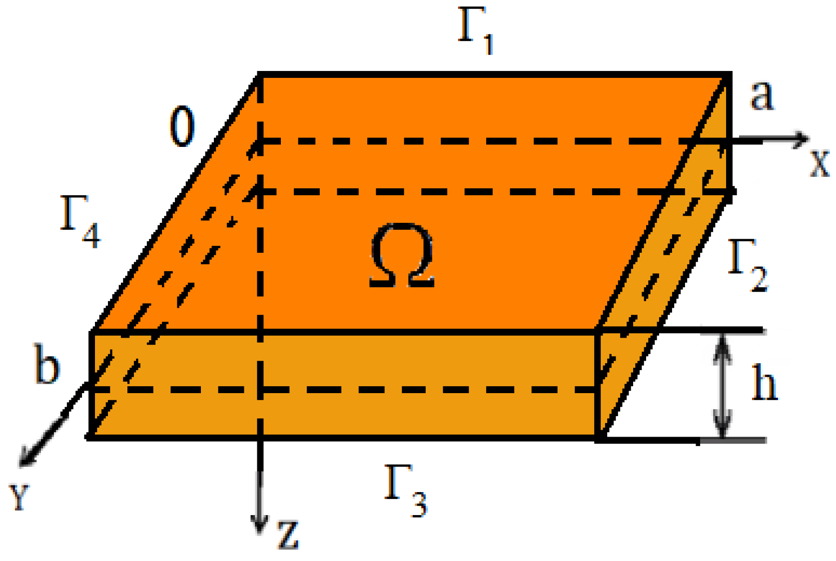
2. Problem Formulation
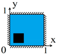
- The accepted classical plate theory (CTP), or Kirchhoff plate theory [16], is widely used in mechanical engineering to analyze the behavior of plates under load. Here, —represents the deflection of the plate’s median plane, which is a function of both x and y, —deformations.
- Physical nonlinearity (FN) is introduced using the deformation theory of plasticity. The material from which the nanoplate is fabricated is considered isotropic but not homogeneous: and —Young’s modulus and the Poisson’s ratio, respectively; —the shear modulus and the bulk modulus depend on coordinates and the strain intensity (8).
- The modified couple stress theory [11] is used to model size-dependent factors. The deformation energy U, taking into account small deformations, is expressed according to the modified couple stress theory [11] as follows:where , , and , , denote the components of the strain tensor and stress tensor, respectively. , , —symmetric part of the curvature tensor; ,,—deviatoric part of the couple stress tensor.
3. Solution Methods
3.1. Application of the Bubnov–Galerkin Method (BGM)
3.2. Application of the Kantorovich–Vlasov Method (KVM)
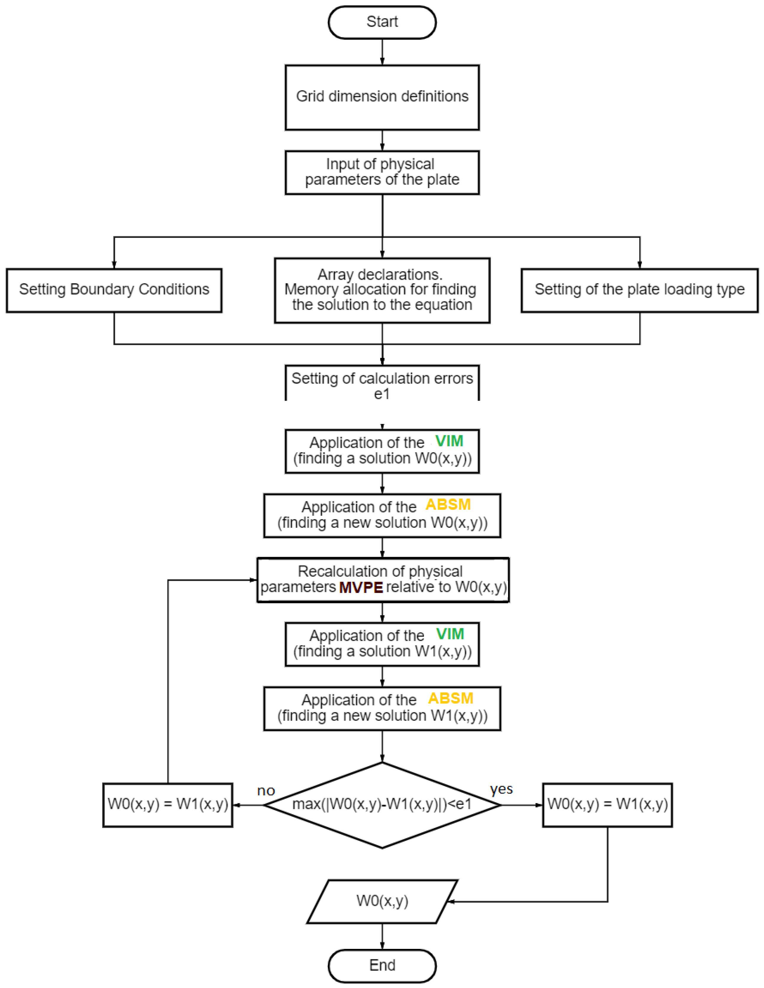
3.3. Application of the Variational Iteration Method (VIM)
4. Numerical Results
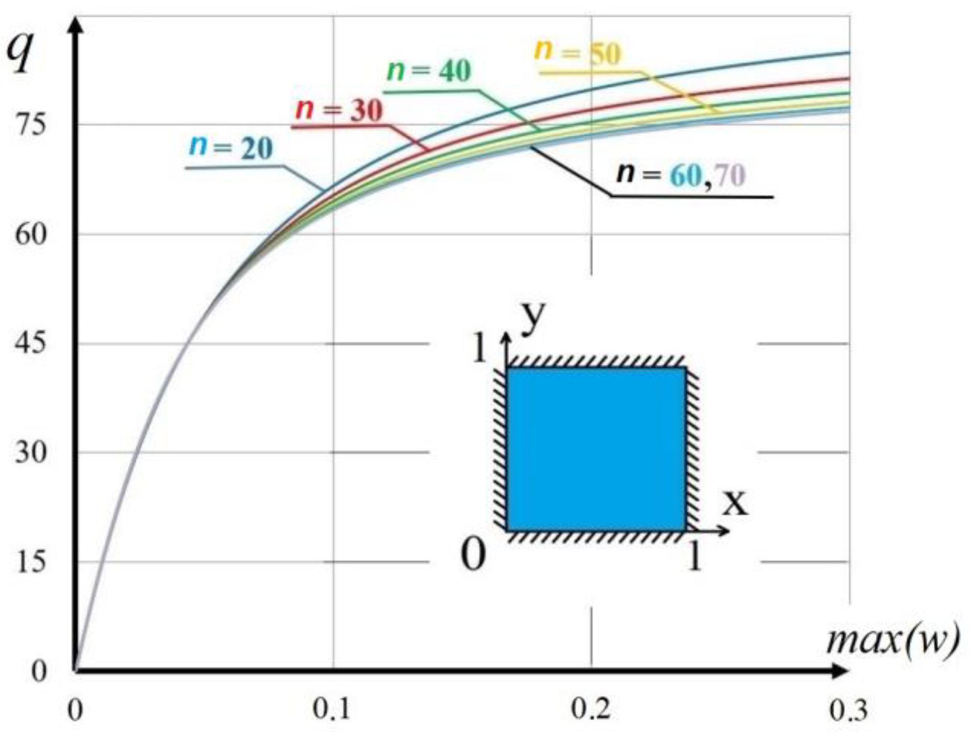
4.1. Methods for Solving the Equation in a Physically Nonlinear Kirchhoff Nanoplate
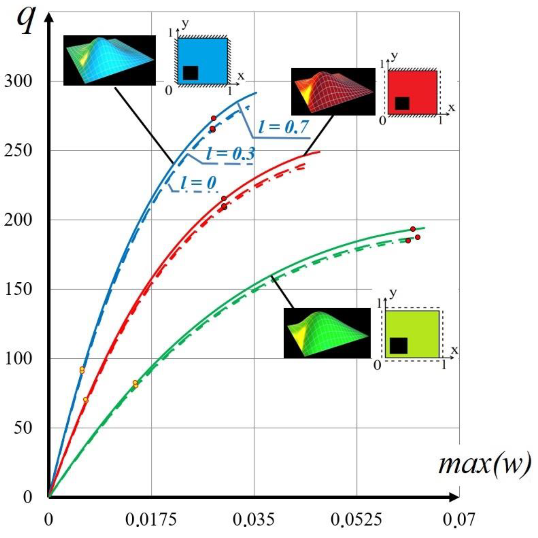
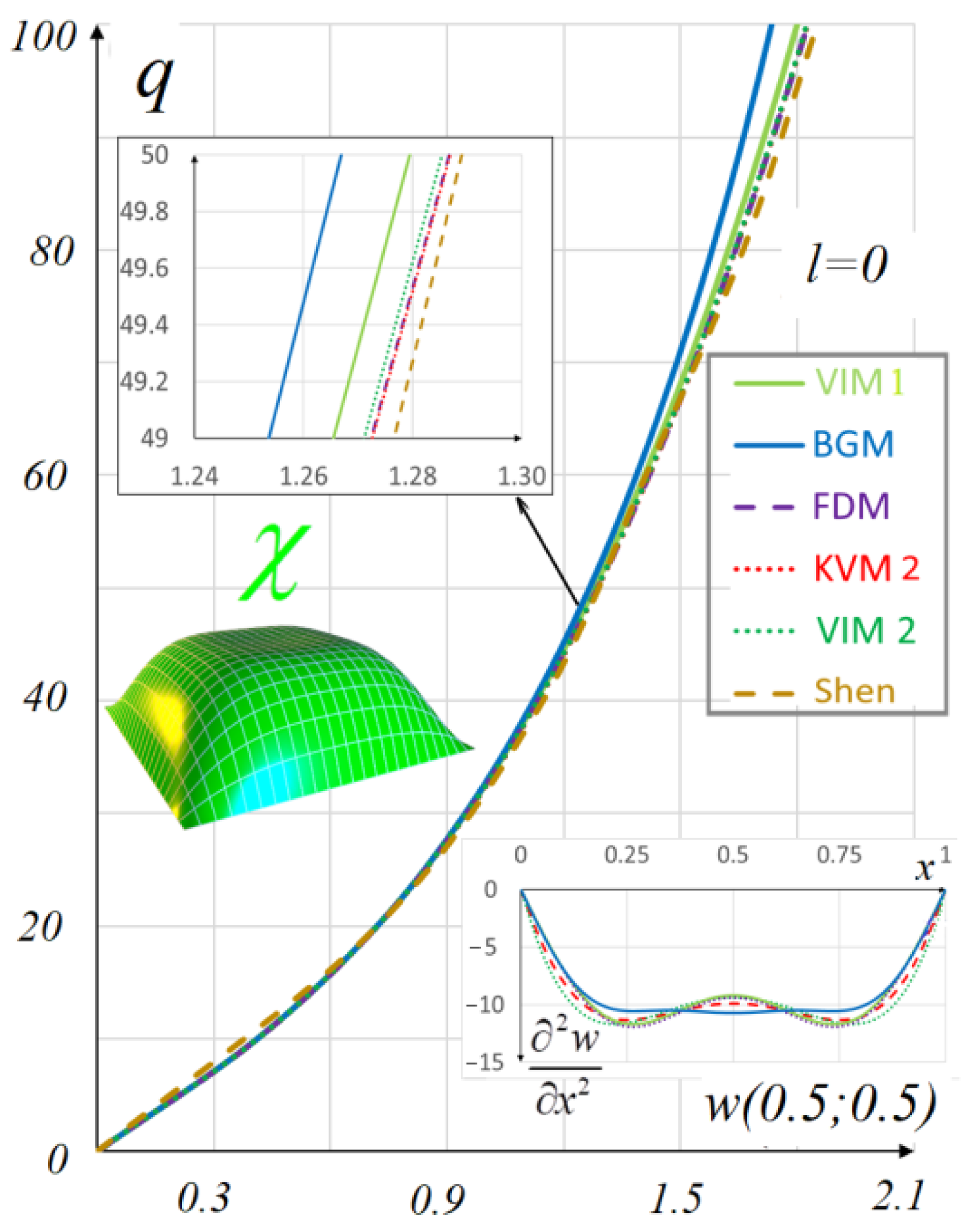
4.2. Methods for Solving the Equation in a Geometrically Nonlinear Kirchhoff Nanoplate
5. Conclusions
Author Contributions
Funding
Data Availability Statement
Conflicts of Interest
References
- Kassir, M. Applied Elasticity and Plasticity, 1st ed.; CRC Press: Boca Raton, FL, USA, 2017; p. 563. [Google Scholar] [CrossRef]
- Molotnikov, V.; Molotnikova, A. Theory of Elasticity and Plasticity: A Textbook of Solid Body Mechanics, 1st ed.; Springer: Berlin/Heidelberg, Germany, 2021; p. 444. [Google Scholar]
- Wang, Z.R.; Hu, W.L.; Yuan, S.J.; Wang, X.S. Engineering Plasticity: Theory and Applications in Metal Forming, 1st ed.; John Wiley & Sons: Hoboken, NJ, USA, 2018; p. 520. [Google Scholar]
- Toupin, R.A. Elastic materials with couple-stresses. Arch. Rational Mech. Anal. 1962, 11, 385–414. [Google Scholar] [CrossRef] [Green Version]
- Mindlin, R.D.; Eshel, N.N. On first strain-gradient theories in linear elasticity. Int. J. Solids Struct. 1968, 4, 109–124. [Google Scholar] [CrossRef]
- Eringen, A.C. Nonlocal polar elastic continua. Int. J. Eng. Sci. 1972, 10, 1–16. [Google Scholar] [CrossRef]
- Eringen, A.C. On differential equations of nonlocal elasticity and solutions of screw dislocation and surface waves. J. Appl. Phys. 1983, 54, 4703–4710. [Google Scholar] [CrossRef]
- Eringen, A. Nonlocal Continuum Field Theories; Springer Science & Business Media: New York, NY, USA, 2002; p. 376. [Google Scholar]
- Shishesaz, M.; Shariati, M.; Yaghootian, A.; Alizadeh, A. Nonlinear Vibration Analysis of Nano-Disks Based on Nonlocal Elasticity Theory Using Homotopy Perturbation Method. Int. J. Appl. Mech. 2019, 11, 1950011. [Google Scholar] [CrossRef]
- Aifantis, E.C. Strain gradient interpretation of size effects. Int. J. Fract. 1999, 95, 299–314. [Google Scholar] [CrossRef]
- Yang, F.; Chong, A.; Lam, D.C.C.; Tong, P. Couple stress based strain gradient theory for elasticity. Int. J. Solids Struct. 2002, 39, 2731–2743. [Google Scholar] [CrossRef]
- Gurtin, M.E.; Murdoch, A.I. Surface stress in solids. Int. J. Solids Struct. 1978, 14, 431–440. [Google Scholar] [CrossRef]
- Liu, Q.; Roy, A.; Silberschmidt, V.V. Size-dependent crystal plasticity: From micro-pillar compression to bending. Mech. Mater. 2016, 100, 31–40. [Google Scholar] [CrossRef] [Green Version]
- Nawaz, A.; Mao, W.G.; Lu, C.; Shen, Y.G. Nano-scale elastic-plastic properties and indentation-induced deformation of single crystal 4H-SiC. J. Mech. Behav. Biomed. Mater. 2017, 66, 172–180. [Google Scholar] [CrossRef]
- Ruocco, E.; Reddy, J.N. Buckling analysis of elastic–plastic nanoplates resting on a Winkler–Pasternak foundation based on nonlocal third-order plate theory. Int. J. Non. Linear Mech. 2020, 121, 103453. [Google Scholar] [CrossRef]
- Awrejcewicz, J.; Krysko-jr., V.A.; Kalutsky, L.A.; Zhigalov, M.V.; Krysko, V.A. Review of the methods of transition from partial to ordinary differential equations: From macro- to nano-structural dynamics. Arch. Comput. Methods Eng. 2021, 28, 4781–4813. [Google Scholar] [CrossRef]
- Kirichenko, V.F.; Krys’ko, V.A. Substantiation of the variational iteration method in the theory of plates. Prikl. Mekhanika 1981, 17, 71–76. (In Russian) [Google Scholar] [CrossRef]
- Krysko, A.V.; Awrejcewicz, J.; Zhigalov, M.V.; Krysko, V.A. On the contact interaction between two rectangular plates. Nonlinear Dyn. 2016, 84, 2729–2748. [Google Scholar] [CrossRef]
- Awrejcewicz, J.; Krysko, V.A.; Zhigalov, M.V.; Krysko, A.V. Contact interaction of two rectangular plates made from different materials with an account of physical non-linearity. Nonlinear Dyn. 2018, 91, 1191–1211. [Google Scholar] [CrossRef] [Green Version]
- Kerr, A.D. An extended Kantorovich method for solution of eigenvalue problem. Int. J. Solid Struct. 1969, 15, 559–572. [Google Scholar] [CrossRef]
- Ansari, R.; Gholami, R. Surface effect on the large amplitude periodic forced vibration of first-order shear deformable rectangular nanoplates with various edge supports. Acta Astronaut. 2016, 118, 72–89. [Google Scholar] [CrossRef]
- Ansari, R.; Gholami, R. Size-dependent modeling of the free vibration characteristics of postbuckled third-order shear deformable rectangular nanoplates based on the surface stress elasticity theory. Compos. Part B Eng. 2016, 95, 301–316. [Google Scholar] [CrossRef]
- Ansari, R.; Mohammadi, V.; Shojaei, M.F.; Gholami, R. Size-dependent postbuckling of annular nanoplates with different boundary conditions subjected to the axisymmetric radial loading incorporating surface stress effects. Int. J. Multiscale Comput. Eng. 2016, 14, 65–80. [Google Scholar] [CrossRef]
- Esmaeilzadeh, M.; Golmakani, M.E.; Kadkhodayan, M.; Amoozgar, M.; Bodaghi, M. Geometrically nonlinear thermo-mechanical analysis of graphene-reinforced moving polymer nanoplates. Adv. Nano Res. 2021, 10, 151–163. [Google Scholar] [CrossRef]
- Gholami, Y.; Gholami, R.; Ansari, R.; Rouhi, H. Size-dependent geometrically nonlinear bending and postbuckling of nanocrystalline silicon rectangular plates based on mindlin’s strain gradient theory. Int. J. Multiscale Comput. Eng. 2019, 17, 583–606. [Google Scholar] [CrossRef]
- Bochkarev, A. On the account of surface tension nonlinearity under of nano-plate bending. Mech. Res. Commun. 2020, 106, 103521. [Google Scholar] [CrossRef]
- Yue, Y.M.; Xu, K.Y.; Tan, Z.Q.; Wang, W.J.; Wang, D. The influence of surface stress and surface-induced internal residual stresses on the size-dependent behaviors of Kirchhoff microplate. Arch. Appl. Mech. 2019, 89, 1301–1315. [Google Scholar] [CrossRef]
- Awrejcewicz, J.; Krysko, V.A., Jr.; Kalutsky, L.A.; Krysko, V.A. Computing static behavior of flexible rectangular von Karman plates in fast and reliable way. Int. J. Non-Linear Mech. 2022, 146, 104162. [Google Scholar] [CrossRef]
- Krysko, V.A., Jr.; Awrejcewicz, J.; Kalutsky, L.A.; Krysko, V.A. Quantification of various reduced order modelling computational methods to study deflection of size-dependent plates. Comput. Math. Appl. 2023, 133, 61–84. [Google Scholar] [CrossRef]
- Alqarni, M.M.; Nasir, A.; Alyami, M.A.; Raza, A.; Awrejcewicz, J.; Rafiq, M.; Ahmed, N.; Shaikh, T.S.; Mahmoud, E.E. A SEIR Epidemic Model of Whooping Cough-Like Infections and Its Dynamically Consistent Approximation. Complexity 2022, 2022, 3642444. [Google Scholar] [CrossRef]
- Ahmed, N.; Macías-Díaz, J.E.; Shahid, N.; Raza, A.; Rafiq, M. A dynamically consistent computational method to solve numerically a mathematical model of polio propagation with spatial diffusion. Comput. Methods Programs Biomed. 2022, 218, 106709. [Google Scholar] [CrossRef]
- Liu, B.; Xing, Y.F.; Eisenberger, M.; Ferreira, A.J.M. Thickness-shear vibration analysis of rectangular quartz plates by a numerical extended Kantorovich method. Compos. Struct. 2014, 107, 429–435. [Google Scholar] [CrossRef]
- Khan, Y.; Tiwari, P.; Ali, R. Application of variational methods to a rectangular clamped plate problem. Comput. Math. Appl. 2012, 63, 862–869. [Google Scholar] [CrossRef] [Green Version]
- Kar, S.; Kumari, P. Three-dimensional analytical solution of arbitrarily supported cylindrical panels with weak interfaces using the extended Kantorovich method. Compos. Struct. 2020, 236, 111802. [Google Scholar] [CrossRef]
- Behera, S.; Kumari, P. Free Vibration Analysis of Levy-Type Smart Hybrid Plates Using Three-Dimensional Extended Kantorovich Method. In Structural Integrity Assessment; Prakash, R., Suresh Kumar, R., Nagesha, A., Sasikala, G., Bhaduri, A., Eds.; Lecture Notes in Mechanical Engineering; Springer: Singapore, 2020. [Google Scholar] [CrossRef]
- Birger, I.A. Some general methods of solution for problems in the theory of plasticity. Prikl. Mat. I Mekhanika 1951, 15, 765–770. (In Russian) [Google Scholar]
- Vorovich, I.I.; Krasovsky, Y.P. On the method of elastic solutions. DAN USSR 1959, 126, 740–743. (In Russian) [Google Scholar]
- Krysko, A.V.; Awrejcewicz, J.; Bodyagina, K.S.; Krysko, V.A. Mathematical modeling of planar physically nonlinear inhomogeneous plates with rectangular cuts in the three-dimensional formulation. Acta Mech. 2021, 232, 4933–4950. [Google Scholar] [CrossRef]
- Krysko, A.V.; Awrejcewicz, J.; Bodyagina, K.S.; Zhigalov, M.V.; Krysko, V.A. Mathematical modelling of physically nonlinear 3D beams and plates made of multimodulus materials. Acta Mech. 2021, 232, 3441–3469. [Google Scholar] [CrossRef]
- Bubnov, I.G. Review of the Work of Prof. S. P. Timoshenko “On the Stability of Elastic Systems”; Selected Works; Sudpromgiz Publishers: Leningrad, Russia, 1956; pp. 136–139. (In Russian) [Google Scholar]
- Galerkin, B.G. Rods and plates. Series in some questions of elastic equilibrium of rods and plates. Bull. Eng. 1915, 1, 897–908. (In Russian) [Google Scholar]
- Kantorovich, L.V.; Krylov, V.I. Approximate Methods of Higher Analysis, 3rd ed.; Benster, C.D., Translator; Interscience: New York, NY, USA, 1959. [Google Scholar]
- Agranovskii, M.L.; Baglai, R.D.; Smirnov, K.K. Identification of a class of nonlinear operators. Zh Vychisl. Mat Mat Fiz 1978, 18, 284–293. (In Russian) [Google Scholar]
- Vlasov, V.Z. General Theory for Shells and Its Application in Engineering; NASA-TT-F-99; National Aeronautics and Space Administration: Washington, DC, USA, 1964; p. 913.
- Mikhlin, S.G. Variational Methods in Mathematical Physics. In International Series of Monographs in Pure and Applied Mathematics, V. 50; Pergamon Press: New York, NY, USA, 1964; p. 583. [Google Scholar]
- Krasnosel’skii, M.A.; Vainikko, G.M.; Zabreiko, P.P.; Rutitskii, Y.B.; Stetsenko, V.Y. Approximate Solution of Operator Equations; Springer: Dordrecht, The Netherlands, 2011; p. 496. [Google Scholar] [CrossRef]
- Kirichenko, V.F.; Krysko, V.A. On the solution of physically nonlinear problems of the theory of plates and shells, rectangular in plan, by the method of variational iterations. Sov. Math. 1982, 26, 104–107. (In Russian) [Google Scholar]
- Ohashi, Y.; Murakami, S. The elasto-plastic bending of a clamped thin circular plate. In Applied Mechanics; Ortler, H.G., Ed.; Springer: Berlin, Heidelberg, 1966; pp. 212–223. [Google Scholar] [CrossRef]
- Kornishin, M.S.; Isanbaeva, F.S. Flexible Plates and Panels; USSR Academy of Sciences: Moscow, Russia, 1968; p. 260. (In Russian) [Google Scholar]
- Shen, H.S. Nonlinear bending of shear deformable laminated plates under transverse and in-plane loads and resting on elastic foundations. Compos. Struct. 2000, 50, 131–142. [Google Scholar] [CrossRef]


| Number of Boundary Condition | Type of Boundary Condition | Load Distributed over the Entire Plane—Type I | Local Load in Third Quarter Plane—Type II |
| (4) |  | 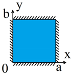 | 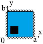 |
| (5) |  | 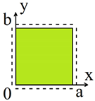 | 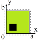 |
| (6) | 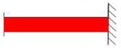 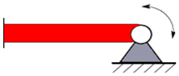 | 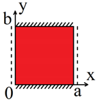 | 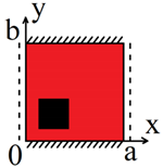 |
| Load-Deflection | Diagrams of Moments |
|---|---|
 | 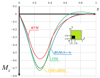 |
| Calculation Methods | Type of Load | ||
|---|---|---|---|
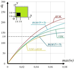
| Type I Uniformly Distributed Load q = 30 | Type II Local Load in the Centre q = 150 | Type III Local Load in the 3rd Quarter q = 130 | |
| Calculation Time, sec. | |||
| BGM (n = 9) | 279.81 | 206.69 | 173.24 |
| BGM (n = 2) | 0.52 | 0.20 | 0.22 |
| KVM | 0.07 | 0.04 | 0.04 |
| VIM | 0.02 | 0.11 | 0.14 |
| VIM + ABSM | 5.02 | 5.01 | 7.97 |
 (3) (3) | ||
| Equal Strain Intensity Lines | Elastic-Plastic Zone Diagrams | |
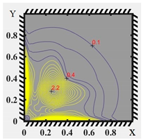 |  | |
 |  | |
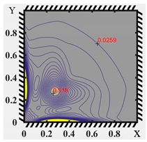 | 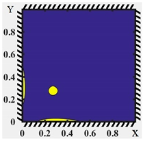 | |
| z | ||
| 205 | 160 | |
| 201 | 120 |
| Method | Error | |
| KVM2 (nx = 25) | 0.9494 | 0.0949 |
| VIM1 (nx = 25) | 0.9473 | 0.1265 |
| VIM2 (n = 25) | 0.9494 | 0.0949 |
| FDM | 0.9524 | 0.4112 |
| FDM | 0.9521 | 0.3795 |
| BGM n = 7 | 0.9485 | 0 |
Disclaimer/Publisher’s Note: The statements, opinions and data contained in all publications are solely those of the individual author(s) and contributor(s) and not of MDPI and/or the editor(s). MDPI and/or the editor(s) disclaim responsibility for any injury to people or property resulting from any ideas, methods, instructions or products referred to in the content. |
© 2023 by the authors. Licensee MDPI, Basel, Switzerland. This article is an open access article distributed under the terms and conditions of the Creative Commons Attribution (CC BY) license (https://creativecommons.org/licenses/by/4.0/).
Share and Cite
Tebyakin, A.D.; Kalutsky, L.A.; Yakovleva, T.V.; Krysko, A.V. Application of Variational Iterations Method for Studying Physically and Geometrically Nonlinear Kirchhoff Nanoplates: A Mathematical Justification. Axioms 2023, 12, 355. https://doi.org/10.3390/axioms12040355
Tebyakin AD, Kalutsky LA, Yakovleva TV, Krysko AV. Application of Variational Iterations Method for Studying Physically and Geometrically Nonlinear Kirchhoff Nanoplates: A Mathematical Justification. Axioms. 2023; 12(4):355. https://doi.org/10.3390/axioms12040355
Chicago/Turabian StyleTebyakin, Aleksey D., Leonid A. Kalutsky, Tatyana V. Yakovleva, and Anton V. Krysko. 2023. "Application of Variational Iterations Method for Studying Physically and Geometrically Nonlinear Kirchhoff Nanoplates: A Mathematical Justification" Axioms 12, no. 4: 355. https://doi.org/10.3390/axioms12040355