Abstract
In industrial production, the exponentially weighted moving average scheme is widely used to monitor shifts in product quality, especially small-to-moderate shifts. In this paper, we propose a modified one-sided EWMA scheme for Type I right-censored Weibull lifetime data for detecting shifts in the scale parameter with the shape parameter fixed. A comparative analysis with existing cumulative sum and exponentially weighted moving average results from the literature is provided. The zero-state and steady-state behaviour of the new scheme are considered with regard to the average run length, the standard deviation of the run length, and other performance measures. Our simulation shows stronger power in detecting changes in the censored lifetime data using the modified scheme than that using the traditional exponentially weighted moving average scheme, and the new scheme is superior to the cumulative sum scheme in most situations. A real-data example further demonstrates the effectiveness of the proposed method.
Keywords:
exponentially weighted moving average; Weibull distribution; censored data; statistical process monitoring MSC:
62P30
1. Introduction
Control charts are widely used as an effective tool in monitoring product quality in industrial production processes. Control charts can be divided into two categories: memoryless control charts and memory-type control charts. Shewhart-type (memoryless) charts, introduced originally by Shewhart [1], have advantages in detecting large shifts but are not sensitive when detecting small shifts. Page [2] and Roberts [3] proposed the cumulative sum (CUSUM) and exponentially weighted moving average (EWMA) procedures, respectively, which make full use of observed data and apply previous information to test statistics, so they are sensitive to small shifts.
In the era of rapid development of information technology and industrial production, high-quality product performance and service are at the core of the sustainable development of enterprises. For instance, Li et al. [4] compared memory-type control charts for monitoring Weibull-distributed time between events, Shafae et al. [5] used CUSUM control charts to monitor Weibull-distributed time-between-event observations, and Chen et al. [6] presented a product reliability-oriented optimization design of the time-between-events control chart system. In recent years, more and more researchers have begun to conduct research on the lifetime and durability of products. For instance, Mukherjee and Marozzi [7] reported the application of control charts to monitor the response times of call centres. Mukherjee et al. [8] applied control charts to the lifetime of a product protected by a warranty from the consumer’s perspective. Product lifetime data are usually restricted by two factors: the data are non-normal and tend to be skewed, and the observed data are often censored. The Weibull distribution, which is widely used in reliability modelling, industrial engineering, and survival studies, was proposed by Weibull [9] to describe material breaking strengths. For instance, the Weibull distribution was applied to describe the strength of carbon fibres in Padgett and Spurrier [10]. Guure and Ibrahim [11] proposed using maximum likelihood and Bayesian estimation methods to estimate the failure rate of the censored Weibull distribution. The failure rate of the Weibull distribution is estimated by a combination of the method of the decreasing function and the Bayesian process in Jiang et al. [12]. Various applications of the Weibull distribution have been studied by Algarni [13], Aslam et al. [14], Mohamed et al. [15], and Al Sobhi [16].
In the actual industrial production process, the observed data are often censored due to time and cost constraints. Scholars have conducted considerable research on the Weibull distribution with censored data. Jia [17] analysed the reliability of the Weibull distribution using maximum likelihood, least-squares, E-Bayesian estimation, and hierarchical Bayesian methods. Steiner and Mackay [18] used the conditional expected value (CEV) to replace censored observed data and then monitored the change in the scale parameter of censored data in Steiner and MacKay [19]. The Weibull extension distribution parameters were estimated under a progressive Type-II censoring scheme with random removal in Almongy et al. [20] for the study of transformer insulation. For the scale parameter of the Weibull distribution with Type I censoring, Zhang and Chen [21] designed two one-sided EWMA CEV charts and Dickinson et al. [22] developed CUSUM control charts. Yu et al. [23] proposed a Shiryaev–Roberts-type scheme for monitoring the scale parameter of the Weibull with Type I censored data. Arif and Aslam [24] transformed Weibull data to normal data and used generally weighted moving average statistics for monitoring. For the shape parameter of the Weibull distribution, the EWMA control charts proposed by Pascual [25] and Pascual and Li [26] used unbiased estimation of the shape parameter to establish a control chart with Type II censored data. Guo and Wang [27] proposed Shewhart-type control charts using the sample range with Type II censored data.
Because EWMA control charts are simple to operate and easy to understand, they are widely used in process monitoring, and many researchers are constantly expanding them. Lucas and Saccucci [28] proposed the Shewhart–EWMA scheme to monitor process means. Sparks et al. [29] improved the EWMA scheme to monitor unusual increases in Poisson counts. Ali et al. [30] proposed the Max-EWMA chart to monitor time and magnitude assuming beta and simplex distributions. Wang et al. [31] used two separate one-sided EWMA t charts to monitor process means using the variable sampling interval (VSI). Malela-Majika et al. [32] proposed a single composite Shewhart–EWMA scheme to monitor the process mean, and Hossain and Riaz [33] designed the V-exponentially weighted moving average (VEWMA) control chart to monitor Maxwell-distributed quality characteristics. To this end, to further improve the performance of the EWMA CEV chart based on the preliminary work of Zhang and Chen [21], inspired by Zhang et al. [34], we propose a parallel modified one-sided EWMA (MOSE) scheme for the censored Weibull distribution in Phase II and compare the new chart with existing control charts in terms of the average run length (ARL) and other indicators. The comparison shows that the proposed control chart is uniformly superior to the EWMA CEV chart under the zero-state case. In the steady-state case, the MOSE chart is better than the existing control charts for monitoring small-to-moderate shifts in the scale parameter when the shape parameter is constant. So, the MOSE control chart is a good choice for practitioners when monitoring small shifts.
This paper is organized as follows. In the next section, we briefly review the properties of the Weibull distribution and EWMA CEV and CUSUM charts. Details about our modified EWMA procedure to monitor the scale parameter of the Weibull distribution with Type I censored data are introduced in Section 3. Section 4 introduces the influence of parameters on the performance of the proposed chart. In Section 5, a comparison with existing methods is given. An example is illustrated in Section 6. Finally, in the last section, conclusions are provided.
2. Related Work
In this section, the mathematical background and properties needed for the design of the MOSE control charts are provided; then, we briefly introduce the EWMA CEV and CUSUM charts proposed by Zhang and Chen [21] and Dickinson et al. [22], respectively.
2.1. Distribution Assumptions
In certain applications, it is common for observational data to be incomplete. There are two types of data censoring: Type I censoring occurs when the process termination time is preset in advance; Type II censoring occurs when the amount of observation data reaches a preset quantity. In this article, we study the Weibull distribution with Type I censoring.
Assume that T has a two-parameter Weibull distribution with shape parameter and scale parameter . Write ; then, the probability density function (pdf) of the failure time T is
and the cumulative distribution function (cdf) is
The mean and variance of T are
respectively, where is the gamma function. In industrial production, more attention is paid to product quality, that is, product life. Since , for fixed , monitoring the decreasing mean is equivalent to detecting a shift in . C and are denoted as the censoring time and censoring rate, respectively. Their relation can be written as
The scale parameter has the same units as T, for example, hours, months, or cycles. The scale parameter indicates the characteristic life of the product; the shape parameter is a unitless number. As Dickinson et al. [22] noted, the scale parameter determines the spread of the distribution, and the shape parameter reflects the specific failure mechanism. When , the Weibull distribution reduces to the traditional exponential distribution, and when , the Weibull distribution closely resembles the normal distribution. In this paper, we assume the parameters and are known for the Phase II monitoring, or which can be estimated by by Phase I data.
In applications, the scale parameter is more likely to change than the shape parameter , as is an inherent parameter and is often fixed. Thus, most existing schemes focus on monitoring the changes in scale parameter by assuming is fixed or equivalently monitoring the distribution mean. To this end, in this paper, we assume the shape parameter is fixed, and then propose a control chart for monitoring the Weibull scale parameter with Type I censored data.
2.2. EWMA CEV Chart Proposed by Zhang and Chen [21]
Zhang and Chen [21] proposed the lower-sided EWMA CEV scheme for monitoring a decrease in with fixed, where Type I right-censored observed data are replaced by the CEV value. Assuming , according to Zhang and Chen [21], sample data are transformed into , then . Based on Steiner and Mackay [18], the censored data can be written by in-control (IC) CEV, namely
Therefore, given a sample of , the transformed variables can be replaced as
Zhang and Chen [21] proposed the following test statistics:
where , and the lower control limit (LCL) os as follows:
where , is the smoothing parameter; is the control limit coefficient; and is a reflecting barrier. Gan [35] proposed the concept of the reflection barrier to improve the inspection performance of the EWMA scheme. The scheme sends an alarm when , where LCL is chosen to achieve a specified IC ARL (ARL).
Similarly, the upper-sided EWMA CEV chart is defined as
where , and the upper control limit (UCL) is defined as
The scheme sends an alarm if , where UCL is chosen to achieve a specified ARL.
2.3. CUSUM Chart Proposed by Dickinson et al. [22]
The CUSUM scheme for monitoring the scale parameter of the Weibull process with Type I censored data was proposed by Dickinson et al. [22]. For right-censored data , Meeker and Escobar [36] applied the following likelihood function:
where if is observed data and if is censored data. Then, Dickinson et al. [22] constructed the CUSUM chart based on the above formula and defined the CUSUM charting statistic:
where can be written as
In Equation (9), suppose in the out-of-control (OOC) case, , where the value of is determined according to the actual situation. When , it means the process mean has increased, and means the process mean has decreased.
According to Dickinson et al. [22], from Equation (9), can be written as
where is the number of actual observed values in the i-th batch . Equivalently, the chart is based on
where . This one-sided CUSUM chart will signal if , where is chosen to achieve a specified ARL.
3. The Proposed Mose Control Chart
The EWMA chart is effective for detecting small-to-moderate shifts. However, if a sudden larger outlier observation occurs at point i and results in , then not all the information of the previous samples is used in the next point. To some extent, this will reduce the efficiency of the scheme. Zhang et al. [34] proposed a modified one-sided EWMA chart, named the MOSE chart, to monitor the process coefficient of variation (CV). This new scheme applied both current and former samples. The simulation comparisons showed that the MOSE scheme was more effective than the traditional one-sided EWMA chart for monitoring the CV. To this end, in this paper, we consider a parallel scheme to monitor Weibull processes under Type I censoring, namely upward and downward shifts in product lifetimes.
Recall that are random variables of Weibull ; when the process is IC, , the downward MOSE chart for each sample 1 can be presented as
where is defined as
where ; ; and is a smoothing parameter. The chart signals when , where LCL is chosen to achieve a specified ARL.
Similarly, the upward MOSE chart for each sample 1 can be presented as
where is defined as
= is the initial value and is the smoothing parameter. The chart signals when , where UCL is chosen to achieve a specified ARL.
When we compare the performance of control charts, the most famous and commonly used statistical measure is ARL. For an IC process, ARL should be sufficiently large to minimize false alarms. For an OOC process, OOC ARL(ARL) should be sufficiently small to detect all shifts in the process rapidly. A control chart is considered better than its competitors if it has a smaller ARL value for a specific shift in the process parameter(s) when ARL is the same for all the charts. In this paper, by means of the R language, we apply Monte Carlo simulation to calculate the run length properties of the control chart. We consider , , and in this comparison. Without loss of generality, for consistency with previous papers by Zhang et al. [34] and Dickinson et al. [22], we set = 1.
For the downward MOSE schemes, the values of the control limits can be calculated via Monte Carlo simulation. In the following, we introduce the control limits and ARL calculation method based on 50,000 replications:
- Step 1.
- Initialize the scenario parameters with the desired values, n, , , and , in the IC process. Select the initial value .
- Step 2.
- Generate a random sample from Weibull according to the above parameters.
- Step 3.
- Step 4.
- Repeat the above steps 50,000 times; the average RL is the ARL corresponding to . Then, adjust the value of using the bisection search method to make the corresponding ARL reach the specified value.
If there is a shift in the process, , shift size represents the percent change with . ARL is used to evaluate the control chart performance and is calculated as follows:
- Step 1.
- Select parameter values: , and h;
- Step 2.
- Step 3.
- If , record the RL; otherwise, go to Step 2;
- Step 4.
- After 50,000 iterations of Step 3–4, ARL is the average of all RL values.
For the upward MOSE schemes, the values of control limits can be calculated by a similar algorithm.
4. Simulation Studies
By means of a simulation algorithm, we study and analyse the effect of two types of data transformation and subsequently investigate the performance of the MOSE control chart, the impact of , and the influence of different shape parameters , censoring rate , and sample size n in the MOSE scheme. The sensitivity analysis of parameter estimation is discussed in this section.
Zero-state ARL (ZS-ARL) and steady-state ARL (SS-ARL) are commonly used to evaluate control chart performance. Zero-state ARL means that the shift occurs at the starting phase of the process, that is, . Steady-state ARL means the process is initially IC but shifts to an OOC state at the change point. In the following study, we assume . For convenience of comparison, we choose ARL = 370 to study the control chart by means of the above iterative algorithm. Each simulation algorithm iterates 50,000 times.
4.1. Comparison of Two Types of Data Transformation
For censored data, most of the literature suggests that the data should be changed to minimize the impact of censoring on the performance of the control chart. Steiner and Mackay [18] suggested that CEV be used instead of the original data for high censoring rates. The data transformation defined in Equation (3) is denoted as Type I data transformation. Another type of data transformation is similar to Equation (5) but replaces with when , and this kind of data transformation is denoted as Type II transformation. Next, we compare the charting performance based on these two types of data transformation.
In this comparison, we choose , , for illustration. By comparing SS-ARL, we can determine the detection performance of the MOSE control chart under two types of data transformation. From Figure 1, we can see that when the censoring rate is small, there is no difference in the performance of the new chart between the two types of data transformation. When the censoring rate is large , the detection performance of the Type I data transformation is significantly better than that of the Type II data transformation. As increases, the difference becomes significant. Therefore, the MOSE chart based on Type I data transformation is constructed in the following comparison.
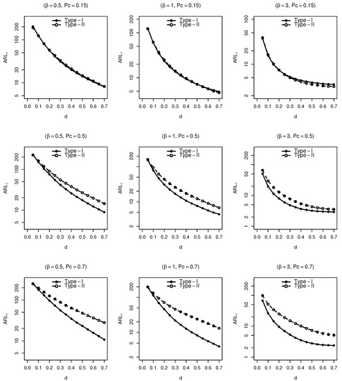
Figure 1.
SS-ARL values for Type I and Type II data transformation .
4.2. Run Length Performance of the MOSE Control Chart
In this part, the performance of the MOSE scheme is reflected by several indicators representing run length characteristics. In addition to ARL, the standard deviation of the run length (SDRL) and the percentiles of the run length distribution, including the 5th, 25th, 50th, 75th, and 95th percentiles, are considered. We take , , and for illustration. In Table 1, we display the attained ARLs, SDRLs, and percentiles (denoted as Q, Q, Q, Q, and Q, respectively). From Table 1, we can observe that all the values decreased with increasing shift magnitude. Under the same shift, SDRLs are less than ARLs, indicating that the proposed chart is relatively stable. For small-to-moderate shifts, the median run length (MRL), i.e., Q, is smaller than the corresponding ARL. For example, when , the ARL is 254.14, and Q is 175. For large shifts, the MRL is close to the corresponding ARL. For instance, when , the ARL and Q are 15.78 and 14, respectively. We also conduct simulations under other parameter combinations and obtain similar results.

Table 1.
SS-ARL, SDRL, and run length quantile values (, , , ).
4.3. The Impact of the Smoothing Parameters
Here, the detectability of the MOSE scheme with different smoothing parameters of is assessed. The MOSE chart is a memory-type chart that combines historical data and current data by means of smoothing parameters. The different choices of smoothing parameters indicate that the weights of historical data are different from those of the current data.
We take = 3, n = 5, and = 0.5 for illustration. Using SS-ARL as the evaluation index, assuming the scale parameter shift , the performance of the MOSE chart under different smoothing parameters is evaluated. In Table 2, as expected, small values of are sensitive to small shifts, while large values of are sensitive to large shifts: the choice of is related to the shift size. In practical applications, we do not know the exact value of the shift, so it is necessary to find the optimal within a shift range. Many indicators can be used to evaluate the performance of the control chart within a certain shift range, such as the extra quadratic loss (EQL), relative average run length (RARL), performance comparison index (PCI), and relative mean index (RMI). These measures are defined in Lu [37] and Han and Tsung [38].
Table 2.
SS-ARL values for the MOSE control chart (ARL = 370, , = 0.5, n = 5).
The EQL can be described as the weighted average of ARL over the process shift range using weight .
where ARL is the ARL value for a specific shift d. In Table 2, = 0.01 to = 0.2; under the same ARL, a smaller EQL represents stronger detection capability.
The RARL is defined as
where ARL and ARL are the ARLs of a specific and the benchmark chart at d, respectively. Generally, the benchmark chart having the minimum values of EQL is measured as RARL = 1.
The PCI value is the ratio given by
where EQL is the lowest EQL of a specific chart.
Han and Tsung [38] proposed the RMI to evaluate performance, defined as
where M is the number of groups in the shift interval. ARL is the value of ARL when the true shift is , and ARL is the smallest ARL when the actual shift is d when takes different data. In Table 2, M = 9, as we use 9 increments from = 0.01 to = 0.2.
The corresponding EQL, RARL, PCI, and RMI values are presented in Table 2. According to the corresponding index, the control chart with smoothing parameter has robust overall performance. For example, is less effective than by 6.13% in terms of the PCI = 1.0613 in Table 2. The RMI values are 3.56%, 17.23% for = 0.05, and 0.15, respectively, and the RMI of is much smaller than that of the other charts.
4.4. The Impact of Different Censoring Rates, Sample Sizes, and Shape Parameters
According to the design procedure of the MOSE chart, the MOSE chart depends on the sample size n, the censoring rate , and the shape parameter . For the parameter combination with sample size n, censoring rate , and shape parameter , the control limit for the MOSE chart computed to achieve the ARL is equal to approximately 370. In practice, the Weibull distribution parameters can be estimated via maximum likelihood estimation. The impact of the smoothing parameter is analysed in the above section. Here, we analyse the impact of the other parameters on the performance of the MOSE chart. We take for illustration. The comparison results are presented in Figure 2, Figure 3 and Figure 4.
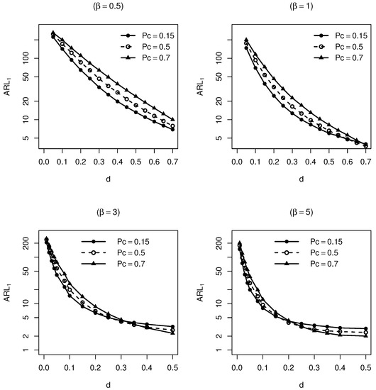
Figure 2.
SS-ARL values for the MOSE chart with different censoring rates ( = 0.1, n = 5).
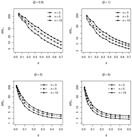
Figure 3.
SS-ARL values for the MOSE chart with different sample sizes n ( = 0.1, = 0.5).
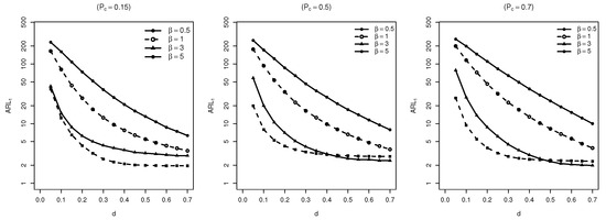
Figure 4.
SS-ARL values for the MOSE chart with different shape parameters ( = 0.1, n = 5).
Figure 2 shows the influence of the censoring rate on the control chart detection performance. We choose and as examples and compare the effects of different censoring rates on the ARL under four cases, . From Figure 2, we can see that as the censoring rate increases, the detectability of the MOSE control chart decreases continuously. This phenomenon is not difficult to understand. The increase in the censoring rate represents a loss of data, and a large loss of accurate data leads to a decline in control chart detectability. Therefore, the relationship between sample size and cost must be balanced in practical applications.
Figure 3 shows the SS-ARL values for the MOSE scheme with different sample sizes n = 3, 5 and 10. We take = 0.5, and = 0.5, 1, 3, 5 in this comparison. An increase in the sample size of each group improves the detection ability of the control chart. Intuitively, an increase in the number of samples provides more information for the control chart, so the control chart can quickly respond to the OOC state.
4.5. Sensitivity Analysis
The control chart described above is established when the Weibull parameters are known. In practice, parameters are often unknown, so we must estimate them. In this part, we discuss the influence of parameter estimation deviation on the proposed chart. We assume the error associated with the parameter estimation is between . When we choose , , = 0.1, and ARL = 370 for the downward shifts in , the control limit is 0.8605. From Table 3, we can see that the bias of both parameters could have a considerable impact on the IC performance of the MOSE control chart. For instance, in Table 3, when = 1, the estimator = 0.9, 0.95, 1, 1.05, 1.1, the ARL values are 94,14, 177.36, 371.41, 810.52, 1791.66, respectively, and the SS-ARL values for detecting the shift of size 0.1 are 32.88, 54.77, 93.26, 164.39, 318.26, respectively, which have considerable differences. When we choose = 1, the estimator = 0.9, 0.95, 1, 1.05, 1.1, the ARL values are 158.97, 237.56, 371.41, 590.6, 968.62, respectively, and the SS-ARL values for detecting the shift in size 0.1 are 55.34, 69.19, 93.26, 120.04, 161.79, respectively. In summary, the parameters and greatly impact the performance of the new chart. Thus, it is necessary to improve the accuracy of parameter estimation to promote the stability of the charting scheme.
Table 3.
Sensitivity analysis based on parameter estimation for downward shifts in . The control limit is produced by the ARL of 370 when , , = 1, = 1, and = 0.1.
5. Comparative Studies
In this part, we compare the new scheme with CUSUM and EWMA CEV and apply Monte Carlo simulation to simulate the ARL under each parameter combination for 50,000 iterations. To facilitate the comparison, we maintain the same parameter settings as the existing methods, that is, , n = 5. Through the comparison of ARL under different parameter combinations, the detection performance of different control charts is explored. We set ARL = 370, , and . The ARL values of the zero state and steady state are shown in the table. We use the same smoothing parameter of for the MOSE and EWMA charts, and the adjustable parameter for the CUSUM chart.
5.1. MOSE versus EWMA CEV
In this section, we compare the MOSE scheme with the EWMA scheme introduced by Zhang and Chen [21]. For the sake of fairness, the values of are consistent with those in Zhang and Chen [21], and four values of are considered.
The results presented in Table 4, Table 5 and Table 6 are under the zero state for . For all four specified smoothing parameters in an OOC situation, the MOSE method is uniformly better than the EWMA CEV for all shifts considered. For example, in Table 4, when = 0.15, = 0.5, and = 0.1, the ZS-ARL values are 146.15, 66.22, 34.54, 20.36, and 13.50 when the shift size d = 0.1, 0.2, 0.3, 0.4, and 0.5, respectively. The corresponding ZS-ARL values for the EWMA CEV chart are 168.31, 78.4, 41.05, 23.73, and 15.16.
Table 4.
ZS-ARL values of the MOSE and existing control charts ( = 1, n = 5, = 0.15).
Table 5.
ZS-ARL values of the MOSE and existing control charts ( = 1, n = 5, = 0.50).
Table 6.
ZS-ARL values of the MOSE and existing control charts ( = 1, n = 5, = 0.70).
For the steady state, the MOSE scheme is superior to the EWMA CEV chart with the same smoothing parameter for small shifts, while the EWMA CEV scheme performs better for large shifts. For instance, in Table 7, when = 5, = 0.15, = 0.1 and d = 0.02, the SS-ARL is 74.72 for the MOSE chart compared with 83.65 for the EWMA CEV, while when d = 0.2, the SS-ARL is 4.23 for the MOSE chart, which is larger than the 3.68 of the EWMA CEV. As increases, the performance of the MOSE decreases.
Table 7.
SS-ARL values of the MOSE and existing control charts ( = 1, n = 5, = 0.15).
The overall conclusions obtained from Table 4, Table 5, Table 6, Table 7, Table 8 and Table 9 are that the MOSE chart is uniformly superior to the EWMA CEV chart under the zero-state case. In the steady-state case, the MOSE chart is better than the EWMA CEV chart for small-to-moderate shifts, while the EWMA chart is slightly better for large shifts.
Table 8.
SS-ARL values of the MOSE and existing control charts ( = 1, n = 5, = 0.50).
Table 9.
SS-ARL values of the MOSE and existing control charts ( = 1, n = 5, = 0.70).
5.2. MOSE versus CUSUM
Here, we compare the MOSE scheme and the CUSUM by ARL. In the comparison of schemes, ARL = 370 and n = 5 are selected as an example, but the two parameters could be set according to the actual situation. We select four values of for the MOSE charts and two values of for the CUSUM for overall performance comparisons.
For the sake of brevity, we choose the adjustment parameter = 0.2 and = 0.1 for comparison. Table 5 shows the results for the zero-state case with = 0.5, and Table 8 shows the results for the steady-state case with = 0.5. When = 3, 5, , the MOSE scheme performs better than the CUSUM scheme, whereas when , the CUSUM scheme outperforms the MOSE scheme. When , the CUSUM scheme is superior to the MOSE when , while the MOSE performs better for large shifts. These findings are consistent with = 0.15 in Table 4 and Table 7 and = 0.7 in Table 6 and Table 9. For example, in Table 4, when = 0.15, = 0.1, = 0.2, and = 3, the ZS-ARL values for the MOSE are 218.31, 131.26, 84.52, 59.91, 43.23, 15.22, and 8.82 when d = 0.01, 0.02, 03, 0.04, 0.05, 0.10, and 0.15, respectively. The ZS-ARL values are 264.2, 195.95, 141.89, 105.65, 79.12, 22.33, and 9.52 for the CUSUM chart. In Table 7, when = 3, 5 and , the MOSE scheme outperforms the CUSUM scheme, especially for small shifts.
All these results show that the MOSE control chart is a good choice for practitioners when monitoring small shifts.
6. Realistic Example
To demonstrate the proposed MOSE scheme, we use the rust test example provided by Steiner and MacKay [19] and also studied by Dickinson et al. [22]. The rust test experiment was designed to observe whether a test unit rusted under a specific environment. Because of the limitation of the cost and time of the experiment, the experiment stipulated the failure time of the test unit to be 20 days. If the panel of the test unit rusted within 20 days, the exact time of rusting was recorded; however, if there was still no rust on the panel on the 20th day, the failure time was recorded as 20 days, that is, the observation value was censored. In this example, the censoring rate is 0.767, and there are 100 subgroups; each group contains 3 data points, and there are 300 observation points in total. According to Lawless [39], Zhang and Chen [21], and Dickinson et al. [22], the parameters in the IC state are estimated to be = 48.04 and = 1.51.
Figure 5 shows the comparison results of the MOSE, CUSUM, and EWMA schemes. According to the assumptions in the previous paper, when ARL = 370, the scale parameter , which decreases by 33%, is detected. The calculation results show that the control limit of the MOSE method is 0.836, and the signal is sent at the 24th sample. The EWMA and CUSUM control charts send alarms at the 24th and 23rd samples, respectively. Observation data and plotting statistics are provided in Table 10. The MOSE control chart is thus shown to be an effective alternative to detect shifts in the scale parameter of a Weibull distribution with Type I censored data.

Figure 5.
CUSUM, EWMA CEV, and MOSE charts for monitoring a 33% decrease in the scale parameter .
Table 10.
Sample number.
7. Conclusions
The scale parameter plays an important role in determining the properties of the Weibull distribution. In monitoring Weibull processes, control charts in the literature often assume that is known and stable. In this paper, we propose a new modified one-sided EWMA chart to monitor changes in Type I right-censored Weibull scale parameter for a fixed value of the shape parameter , which is equivalent to monitoring the mean of a Weibull process. The new one-sided EWMA chart takes into account all the historical data information up to the current time point. The simulation results reveal that the performance of the proposed chart and the other two existing charts depend on the value of the fixed shape parameter, censoring rate and sample size. The parameters can be set according to the actual situation in practical applications. It has also been shown that the three charts take longer to detect a decrease in the scale parameter when the shape parameter is small. By contrast, larger values of the shape parameter lead to faster detection. The MOSE chart performs well in detecting decreases in the scale parameter and performs better than the traditional EWMA CEV chart in many of the scenarios considered. Compared with the CUSUM chart, the MOSE chart performs better for specific parameter values . The sensitivity analysis shows that the performance of the MOSE chart depends on the parameter estimation, and the deviation of the parameter estimation influences the stability of the proposed scheme.
The focus of this paper is to detect decreases in the scale parameter, but it is also possible to monitor increases in the scale parameter using the one-sided upper EWMA statistics given in Equations (13) and (14). In future development, the current study can be extended using Neutrosophic statistics, which have been studied in Aslam and Arif [40], AlAita and Aslam [41], and Smarandache [42]. Another important direction of future research is to extend the proposed procedure when standards are unknown and estimated from a reference sample.
Author Contributions
Conceptualization, D.Y., L.J., J.L., X.Q., Z.Z. and J.Z.; methodology, D.Y. and L.J.; software, D.Y. and J.L.; validation, D.Y., L.J., J.L., X.Q., Z.Z. and J.Z.; formal analysis, D.Y.; writing—original draft preparation, D.Y.; writing—review and editing, D.Y., L.J. and J.L.; supervision, D.Y., L.J., J.L., X.Q., Z.Z. and J.Z.; project administration, D.Y.; funding acquisition, D.Y., Z.Z. and J.Z. All authors have read and agreed to the published version of the manuscript.
Funding
This research was supported by the General Program of the Natural Science Foundation of Liaoning Province (No.2020-MS-139), the Project of Science and Research of Liaoning Educational Department of China (No.LJC202006), the Natural Science Foundation of Liaoning Province, (No.2023-MS-142), the Doctoral Research Start-up Fund of Liaoning Province [grant number 2021-BS-142], the National Natural Science Foundation of China [grant number 12201429], the Research on Humanities and Social Sciences of the Ministry of Education (22YJC910009), the Research of economic and social development in Liaoning Province (grant number 20231s1ybkt-103).
Data Availability Statement
All data are available in the paper.
Conflicts of Interest
The authors declare that there are no conflict of interest regarding the publication of this paper.
References
- Shewhart, W.A. Economic Control of Quality of Manufactured Product; Macmillan and Co. Ltd.: London, UK, 1931. [Google Scholar]
- Page, E. Continuous inspection schemes. Biometrika 1954, 41, 100–115. [Google Scholar] [CrossRef]
- Roberts, S. Control chart tests based on geometric moving averages. Technometrics 1959, 1, 239–250. [Google Scholar] [CrossRef]
- Li, J.; Yu, D.; Song, Z.; Mukherjee, A.; Chen, R.; Zhang, J. Comparisons of some memory-type control chart for monitoring Weibull-distributed time between events and some new results. Qual. Reliab. Eng. Int. 2022, 38, 3598–3615. [Google Scholar] [CrossRef]
- Shafae, M.S.; Dickinson, R.M.; Woodall, W.H.; Camelio, J.A. Cumulative sum control charts for monitoring Weibull-distributed time between events. Qual. Reliab. Eng. Int. 2015, 31, 839–849. [Google Scholar] [CrossRef]
- Chen, Z.; He, Y.; Cui, J.; Han, X.; Zhao, Y.; Zhang, A.; Zhou, D. Product reliability–oriented optimization design of time-between-events control chart system for high-quality manufacturing processes. Proc. Inst. Mech. Eng. Part D J. Eng. Manuf. 2020, 234, 549–558. [Google Scholar] [CrossRef]
- Mukherjee, A.; Marozzi, M. A distribution-free phase-II CUSUM procedure for monitoring service quality. Total Qual. Manag. Bus. Excell. 2017, 28, 1227–1263. [Google Scholar] [CrossRef]
- Mukherjee, A.; Mccracken, A.K.; Chakraborti, S. Control Charts for Simultaneous Monitoring of Parameters of a Shifted Exponential Distribution. J. Qual. Technol. 2015, 47, 176–192. [Google Scholar] [CrossRef]
- Weibull, W. A statistical theory of the strength of materials. Swed. R. Inst. Eng. Res. 1939, 151, 1–45. [Google Scholar]
- Padgett, W.; Spurrier, J. Shewhart-type charts for percentiles of strength distributions. J. Qual. Technol. 1990, 22, 283–288. [Google Scholar] [CrossRef]
- Guure, C.B.; Ibrahim, N.A. Bayesian analysis of the survival function and failure rate of Weibull distribution with censored data. Math. Probl. Eng. 2012, 2012, 329489. [Google Scholar] [CrossRef]
- Jiang, P.; Xing, Y.; Jia, X.; Guo, B. Weibull failure probability estimation based on zero-failure data. Math. Probl. Eng. 2015, 2015, 681232. [Google Scholar] [CrossRef]
- Algarni, A. Group Acceptance Sampling Plan Based on New Compounded Three-Parameter Weibull Model. Axioms 2022, 11, 438. [Google Scholar] [CrossRef]
- Aslam, M.; Jeyadurga, P.; Balamurali, S.; Khan Sherwani, R.A.; Albassam, M.; Jun, C.H. A New Variable-Censoring Control Chart Using Lifetime Performance Index under Exponential and Weibull Distributions. Comput. Intel. Neurosci. 2021, 2021, 1350169. [Google Scholar] [CrossRef] [PubMed]
- Mohamed, R.A.; Tolba, A.H.; Almetwally, E.M.; Ramadan, D.A. Inference of Reliability Analysis for Type II Half Logistic Weibull Distribution with Application of Bladder Cancer. Axioms 2022, 11, 386. [Google Scholar] [CrossRef]
- Al Sobhi, M.M. The extended Weibull distribution with its properties, estimation and modeling skewed data. J. King Saud Univ. Sci. 2022, 34, 101801. [Google Scholar] [CrossRef]
- Jia, X. Reliability analysis for Weibull distribution with homogeneous heavily censored data based on Bayesian and least-squares methods. Appl. Math. Model. 2020, 83, 169–188. [Google Scholar] [CrossRef]
- Steiner, S.; Mackay, R. Monitoring processes with highly censored data. J. Qual. Technol. 2000, 32, 199–208. [Google Scholar] [CrossRef]
- Steiner, S.; MacKay, R. Detecting changes in the mean from censored lifetime data. Front. Stat. Qual. Control 6 2001, 3, 275–289. [Google Scholar]
- Almongy, H.M.; Alshenawy, F.Y.; Almetwally, E.M.; Abdo, D.A. Applying transformer insulation using Weibull extended distribution based on progressive censoring scheme. Axioms 2021, 10, 100. [Google Scholar] [CrossRef]
- Zhang, L.; Chen, G. EWMA Charts for Monitoring the Mean of Censored Weibull Lifetimes. J. Qual. Technol. 2004, 36, 321–328. [Google Scholar] [CrossRef]
- Dickinson, R.; Roberts, D.; Driscoll, A.; Woodall, W.; Vining, G. CUSUM Charts for Monitoring the Characteristic Life of Censored Weibull Lifetimes. J. Qual. Technol. 2014, 46, 340–358. [Google Scholar] [CrossRef]
- Yu, D.; Mukherjee, A.; Li, J.; Jin, L.; Wen, K.; Zhang, J. Performance of the Shiryaev-Roberts-type scheme in comparison to the CUSUM and EWMA schemes in monitoring weibull scale parameter based on Type I censored data. Qual. Reliab. Eng. Int. 2022, 38, 3379–3403. [Google Scholar] [CrossRef]
- Arif, O.H.; Aslam, M. A new generalized range control chart for the Weibull distribution. Complexity 2018, 2018, 9453589. [Google Scholar] [CrossRef]
- Pascual, F. EWMA Charts for the Weibull Shape Parameter. J. Qual. Technol. 2010, 42, 400–416. [Google Scholar] [CrossRef]
- Pascual, F.; Li, S. Monitoring the Weibull shape parameter by control charts for the sample range of type II censored data. Qual. Reliab. Eng. Int. 2012, 28, 233–246. [Google Scholar] [CrossRef]
- Guo, B.; Wang, B.X. Control Charts For Monitoring The Weibull Shape Parameter Based On Type-II Censored Sample. Qual. Reliab. Eng. Int. 2012, 30, 13–24. [Google Scholar] [CrossRef]
- Lucas, J.; Saccucci, M. Exponentially weighted moving average control schemes: Properties and enhancements. Technometrics 1990, 32, 1–12. [Google Scholar] [CrossRef]
- Sparks, R.S.; Keighley, T.; Muscatello, D. Improving EWMA plans for detecting unusual increases in Poisson counts. Adv. Decis. Sci. 2009, 2009, 512356. [Google Scholar] [CrossRef][Green Version]
- Ali, S.; Akram, M.F.; Shah, I. Max-EWMA Chart Using Beta and Simplex Distributions for Time and Magnitude Monitoring. Math. Probl. Eng. 2022, 2022, 7306775. [Google Scholar] [CrossRef]
- Wang, Y.; Hu, X.; Zhou, X.; Qiao, Y.; Wu, S. New One-Sided EWMA t Charts without and with Variable Sampling Intervals for Monitoring the Process Mean. Math. Probl. Eng. 2020, 2020, 7567215. [Google Scholar] [CrossRef]
- Malela-Majika, J.C.; Shongwe, S.C.; Castagliola, P.; Mutambayi, R.M. A novel single composite Shewhart-EWMA control chart for monitoring the process mean. Qual. Reliab. Eng. Int. 2022, 38, 1760–1789. [Google Scholar] [CrossRef]
- Hossain, M.P.; Riaz, M. On designing a new VEWMA control chart for efficient process monitoring. Comput. Ind. Eng. 2021, 162, 107751. [Google Scholar] [CrossRef]
- Zhang, J.; Li, Z.; Chen, B.; Wang, Z. A new exponentially weighted moving average control chart for monitoring the coefficient of variation. Comput. Ind. Eng. 2014, 78, 205–212. [Google Scholar] [CrossRef]
- Gan, F. Exponentially weighted moving average control charts with reflecting boundaries. J. Stat. Comput. Simul. 1993, 46, 45–67. [Google Scholar] [CrossRef]
- Meeker, W. Statistical Methods for Reliability Data; Wiley: Hoboken, NJ, USA, 1998. [Google Scholar]
- Lu, S.L. Non parametric double generally weighted moving average sign charts based on process proportion. Commun. Stat. Theory Methods 2018, 47, 2684–2700. [Google Scholar] [CrossRef]
- Han, D.; Tsung, F. A reference-free cuscore chart for dynamic mean change detection and a unified framework for charting performance comparison. J. Am. Stat. Assoc. 2006, 101, 368–386. [Google Scholar] [CrossRef]
- Lawless, J.F. Statistical Models and Methods for Lifetime Data; John Wiley & Sons: Hoboken, NJ, USA, 2011. [Google Scholar]
- Aslam, M.; Arif, O.H. Testing of grouped product for the weibull distribution using neutrosophic statistics. Symmetry 2018, 10, 403. [Google Scholar] [CrossRef]
- AlAita, A.; Aslam, M. Analysis of covariance under neutrosophic statistics. J. Stat. Comput. Simul. 2022, 93, 397–415. [Google Scholar] [CrossRef]
- Smarandache, F. Introduction to Neutrosophic Sociology (Neutrosociology); Infinite Study; The University of New Mexico: Albuquerque, NM, USA, 2019. [Google Scholar]


Disclaimer/Publisher’s Note: The statements, opinions and data contained in all publications are solely those of the individual author(s) and contributor(s) and not of MDPI and/or the editor(s). MDPI and/or the editor(s) disclaim responsibility for any injury to people or property resulting from any ideas, methods, instructions or products referred to in the content. |
© 2023 by the authors. Licensee MDPI, Basel, Switzerland. This article is an open access article distributed under the terms and conditions of the Creative Commons Attribution (CC BY) license (https://creativecommons.org/licenses/by/4.0/).