Characterization of Aeroelastic Behavior in a High Aspect Ratio Wing Using Computational and Wind Tunnel Experiments

Abstract

The objective of this article is to characterize an aeroelastic system in terms of its dynamical behavior, which could be either chaotic or periodic before, during, and after achieving the flutter velocity. The aeroelastic system shown here is a wing with a high aspect ratio, which leads to a very flexible behavior subjected to unsteady flow. This paper compares the computational and experimental dynamical behavior of an aeroelastic system at the flutter velocity for the different dynamic stall models proposed. To understand the nonlinear behavior of this system, the traditional attractor reconstruction and Lyapunov exponent calculation are compared with the 0–1 test. In addition to this comparison, two dynamic stall semi-empirical models are applied directly to the time history. All these comparisons show that the computational and wind tunnel experiments are in good agreement, and the dynamic behavior usually gives close results for the 0–1 test and Lyapunov exponent. It is concluded that the system presents chaotic behavior when no dynamic stall correction is applied or when Gangwani’s correction is applied. However, Boeing–Vertol’s correction postpones the chaotic behavior, meaning that the chaotic behavior is only observed for velocities above the flutter.

1. Introduction

The search for more environmentally friendly aircraft is a real concern these days, and one way to reduce aircraft gas emissions is by reducing fuel consumption, which can be effectively done by reducing drag. One of the most effective ways to reduce drag is to increase the aspect ratio of wings with lighter solutions. More flexible wings lead to geometric nonlinearities. One example of geometric nonlinearity presence is airplanes with high altitude and long endurance, which are extremely flexible [1,2].

Investigations on aeroelastic wings have attracted the attention of many researchers in recent years [3]. According to [4], the aeroelastic phenomena in the wings can interfere with the design and performance of the aircraft [4]. To analyze the aeroelastic phenomena of the wing, Ref [5] presents a set of solution algorithms for nonlinear multiparameter eigenvalue problems that occur in the analysis of flutter. Meanwhile, Ref. [6] presents a fast static aeroelastic analysis approach that incorporates the modal method. In [7], a modified harmonic balancing approach is presented to study the nonlinear aeroelastic behavior of a two-degree-of-freedom (DOF) airfoil. In [8], aerodynamic analyses are presented in an aeroelastic system, including coupled nonlinearities in the system, and the dynamic stall effects resulting from large instantaneous angles of attack are included in the investigation. The nonlinearities inherent in aeroelastic systems enrich the dynamics of the system to have Hopf bifurcations and chaotic behavior [9,10]. In [11], the nonlinear aeroelastic response is performed using a wing-based system with two DOFs in the presence of quadratic and cubic nonlinearities in the pitch DOF.

This paper will present the effect of geometric nonlinearities in terms of dynamic aeroelasticity [12]. Aeroelasticity is the Engineering field that studies how elastic, inertial, and aerodynamic forces interact with each other. The main topics discussed in Aeroelasticity are flutter, gust response, and buffeting, for example. Aeroelastic problems can be observed not only in aircraft but in bridges (Tacoma Narrow’s bridge, for example, which is a classical flutter example), buildings, pipelines for oil extraction below the sea, etc. Since the beginning of aircraft history, Aeroelasticity has been present. Flutter is an auto-excited dynamic aeroelasticity phenomenon and occurs when the unsteady aerodynamic forces acting on a system lead to the coupling of two or more vibration modes. High aspect ratio wings are more easily observed these days. As stated before, the main motivation is to reduce drag, which reduces fuel consumption, and today, it is possible to use composite materials to increase aspect ratio, tailoring the aeroelastic characteristics and optimize weight gain. Commercial aircraft today are good examples, such as the Boeing 787 Dreamliner and HALE (high altitude long endurance) aircraft, which are used in different research. High aspect ratio wings, like helicopter blades, tend to present geometrical nonlinearities, as the one presented in this paper. Also, helicopter blades present dynamic stall, and with that in mind, this paper will present an initial approach to it, using semi-empirical methods.

The case to be presented here is a high aspect ratio wing with a slender body at the wing tip. This slender body was specially designed to reduce the flutter speed by reducing the frequency of the first torsion mode. The main idea behind reducing the flutter speed is to test this aeroelastic model in any available subsonic wind tunnel [13]. The resulting flutter mechanism is the classical bending-torsion aeroelastic mode, observed in most actual aircraft in the world and which shall be avoided in the aircraft flight envelope. This wing was designed to present a flutter velocity within the speed range of the wind tunnel [13]. Also, the model should be simple and easy to build and reproduce whenever needed [14]. The aeroelastic system shown in this paper is different from that of a flat plate, presented before by the authors ([14,15]). A similar study introducing the procedures presented here, but with a typical section with airfoil NACA 0012 and three degrees of freedom, is present in [16]. After the aeroelastic model is designed using traditional commercial software, such as NASTRAN^® and ZAERO^®, it shall be built and tested in the wind tunnel.

During the wind tunnel tests, the model did not collapse, as expected to occur during a traditional flutter, which is a destructive and explosive phenomenon. Additionally, during wind tunnel tests, the model shows large visual vibration-like deformations every time the flutter speed is achieved. This deformation possibly induces a dynamic stall phenomenon, especially near the tip of the wings. Two different dynamic stall semi-empirical models are used: Boeing–Vertol [17] and Gangwani [18]. Dynamic stall is a phenomenon mainly observed in helicopter blades and occurs when a certain angle of attack is achieved, and the flow starts to detach from the aerodynamic surface, causing an abrupt reduction of the lift force. This nonlinear aerodynamic phenomenon leads to a common aeroelastic phenomenon known as stall flutter. The unsteadiness of the flow caused by the pitch and plunge movements is what distinguishes the static stall from the dynamic stall. This unsteadiness causes a delay in the moment that the stall is usually predicted by linear theories, leading to an overshoot in lift and aerodynamic moment [19]. The main causes of dynamic stall are: (1) unsteady flow caused at the moment a vortex moves upstream of the trailing edge wake, (2) airfoil pitch rate kinematics (pitch rate due to time), and (3) additional unsteady effects within the boundary layer, such as reverse flow. Boeing–Vertol [17] and Gangwani [18] models calculate corrections to be applied to the aerodynamic coefficients CL (lift coefficient) and CM (aerodynamic pitch moment coefficient). The dynamic stall is a complex phenomenon, and more dedicated research is recommended for this case study. Usually, high-fidelity CFD-based methodologies are better used to predict the dynamic stall. However, the computational cost is too high, and considering this paper’s goals, it does not make sense to invest such effort. This is the reason to apply semi-empirical methods that only calculate a factor necessary to be applied in forces and moments to adjust them for the stall (the same factor is linearly applied in all sections along the span, and the same technique is used in some other flutter analyses to capture other nonlinear effects).

The experimental aeroelastic analysis is presented using dynamics tools, like PSD (power spectral density) [20], which is also recommended for nonlinear systems [1,21,22,23]. To verify the dynamic behavior of the time series of an aeroelastic system, the 0–1 test is performed [24], which is a method to verify whether a phenomenon has chaotic behavior from a certain time series [25]. Additionally, the Lyapunov exponent is calculated, and the attractor is reconstructed using Takens’ theory [26] to be compared with the results of the 0–1 test. All these methodologies do not need prior knowledge of the dynamic systems equation and can be applied directly to a certain time history, which is ideal for complex experiments with uncertainties related to the boundary conditions (attachment and wind tunnel boundary layer influence). The same procedure is performed but with the computational time series obtained from a nonlinear geometric formulation based on strain combined with the unsteady aerodynamic formulation (Peters’ model, commonly used in helicopter aeroelastic analysis). Semi-empirical dynamic stall methodologies are applied only for computational results ([17,18]), which are then compared with experimental wind tunnel results.

One motivation is related to the aeroelastic wind tunnel model of this paper. Wind tunnel flutter tests were performed and presented in [13], in which commercial software was used in flutter prediction before the experiments, which considered only linear theory. Since the observed dynamics were different from those predicted by linear theory, this system might present some nonlinearity. Since shock waves cannot occur (low subsonic and zero angle of attack), dynamic stall might be a possibility. However, the model presents a high aspect ratio and high flexibility, and the structural nonlinearity seems to be more likely to dominate over the aerodynamic effects.

Another motivation for this research is that the formulation known as the 0–1 test for chaos is a fast tool to know if a test result presents chaotic behavior or nonlinear but periodic behavior from the time history of an experiment without the dynamic system equation [24]. This test is not usual for aeroelastic systems in a post-flutter analysis, but its applicability as a test for chaos for dynamical systems is treated by [27].

The main contribution of this paper is to show the importance of analyzing the nonlinear dynamic behavior of a highly geometric nonlinear system and to verify the possibility of applying the 0–1 test to classify between periodic or chaotic behavior of an aeroelastic system subject to high deformations. If the result of the 0–1 test agrees well with traditional attractor reconstruction and Lyapunov exponent calculation, it could be applied to the aeroelastic wind tunnel and the computational results directly using time series. For aircraft applications, depending on the amplitude oscillations, the wings shall be re-designed. Chaos, although it is not a problem, might lead to sudden high amplitudes that result in structure collapse. Advances in this research could prevent undesirable phenomena [28].

The aeroelastic model used in this paper is more flexible than the model presented in [14], so it presented higher deformations and a possible effect of dynamic stall, as demonstrated in the results (Section 4).

This paper is organized into the following sections. Section 2 presents all the theoretical background necessary for the developments shown afterward. The third Section presents the experiment in terms of model and wind tunnel characteristics. Section 4 presents the results for the computational experiments, considering before, during, and after the flutter onset and the wind tunnel experiment at the flutter velocity. Finally, the concluding remarks and topics for future research are shown in Section 5, and the list of main references is used.

2. Theoretical Background

The following subsections will briefly present the theoretical background of the strain-based geometrically nonlinear formulation used to obtain the time series of computational experiments. The dynamic stall correction methods are also presented here and shall be applied to the time series obtained previously (results in Section 4). The theoretical background of the 0–1 test for chaos and the phase-space reconstruction based on Takens’ theory are shown, as well as the Lyapunov exponent related to each attractor.

2.1. Strain-Based Geometrically Nonlinear Formulation

This subsection’s objective is to briefly present the theoretical background used in this research to obtain the time series for the computational experiments before the dynamic stall correction. With these time series, the dynamic stall CL and CM are calculated, and this framework is performed again, considering the correction. The results with and without correction are presented in Section 4.

The strain-based geometrically nonlinear formulation [29] is developed in the MATLAB^® environment and can be found in [16]. This framework performs aeroelastic analysis considering geometric nonlinearities. In this subsection, only a few implemented equations are presented for brevity, and more details on this formulation can be found in Cardoso-Ribeiro [29]. The formulation presented here is based on an energy approach considering deformations in bending (out-of-plane and in-plane), torsion, and extension, so it can be applied to large displacements, as expected to happen with very flexible structures subjected to unsteady aerodynamic forces. These forces are calculated using the strip theory based on the unsteady Peters’ model [29].

The virtual work principle is applied to determine the dynamic equation of the system [29]. The wing (or aircraft, depending on the case) is modeled using nonlinear beam elements, and the structural dynamics formulation considers the deformation as a generalized coordinate (both bending, torsion, and extension, which gives nonlinear behavior to the structure). The wing presented in this paper is modeled as a one-dimensional beam with certain characteristics of the transverse section [29]. The nonlinear equation of motion is [16]

$$M\left(\epsilon \right)\ddot{\epsilon }+C(\epsilon ,\dot{\epsilon })\dot{\epsilon }+K\left(\epsilon \right)\epsilon =R,$$

(1)

where

$$M\left(\epsilon \right)=J_{h\epsilon }^{T}M{J}_{h\epsilon },$$

(2)

$$C\left(\epsilon ,\dot{\epsilon }\right)=J_{h\epsilon }^{T}M{\dot{J}}_{h\epsilon }+C$$

(3)

$$K\left(\epsilon \right)=K$$

(4)

$$R=J_{p\epsilon }^T{F}_{pt}+J_{\theta \epsilon }^T{M}_{pt}+J_{p\epsilon }^T{B}^F{F}_{dist}+J_{\theta \epsilon }^T{B}^M{M}_{dist}$$

(5)

In Equations (2)–(4), $M$, $C$, and $K$ are structural mass, damping, and stiffness, respectively. The Jacobian matrices $J_{h\epsilon }$, $J_{p\epsilon ,}$ and $J_{\theta \epsilon }$ expressed in Equations (2), (3) and (5) relate the structural deformations to the translation and rotation of each node. The Jacobian matrices are a function of the deformation vector $\epsilon$ [29], which expresses geometric nonlinearity. The forces and moments acting on the aeroelastic system are represented by $R$ in Equation (5), where the $pt$ is for punctual or concentrated forces and moments, and the subscript $dist$ for distributed. In this case of study, $R$ is the total aerodynamic force (lift) and moment, which are given by the unsteady aerodynamic model [29]:

$$L=\pi \rho b^2\left(-\ddot{z}+\dot{y}\dot{\alpha }-ab\ddot{\alpha }\right)+2\pi \rho b{\dot{y}}^2\left[-\frac{\dot{z}}{\dot{y}}+b\left(0.5-a\right)\frac{\dot{\alpha }}{\dot{y}}-\frac{{\lambda }_0}{\dot{y}}\right]$$

(6)

$$M_{ea}=Lab+2\pi \rho b^2\left(-\frac{1}{2}\dot{y}\dot{z}-\frac{1}{2}ab\dot{y}\dot{\alpha }-\frac{1}{2}\dot{y}{\lambda }_0-\frac{1}{16}{b}^2\ddot{\alpha }\right)$$

(7)

where $\rho$ is the air density, b is the half-chord length, a is the position of the aerodynamic center relative to the elastic axis, $\dot{\alpha }$ is the pitch rate, ${\lambda }_0$ is the lag term, y is the axis parallel to the airfoil zero lift line, and z is perpendicular upwards, which are the definitions of the variables and are traditionally used in everyday unsteady aerodynamic analysis with this nomenclature. Equations (6) and (7) calculate the lift and aerodynamic moment for each panel of the model. For the case presented in this paper, 10 aerodynamic elements are used (after a convergence analysis, no more than 10 are necessary), and the flutter velocity calculated by this method agrees with the wind tunnel measurement. It is important to highlight that even commercial software uses panel methods in flutter analysis, and the results are in good agreement with experimental data when no aerodynamic nonlinearities are present, like shock waves. For a small disturbance context, such as flutter, panel methods give as good results as fluid-structure interaction.

With the advent of helicopters and the study of tilt-wing and tilt-rotor configurations, different methodologies [19] to estimate the dynamic stall have been studied. Considering the present objectives of this research, it is more suitable to apply semi-empirical methods to estimate the correction needed for CL and CM (aerodynamic forces and moments) to adjust them for dynamic stall. During the wind tunnel tests, high-amplitude oscillations are expected, so this phenomenon could occur at flutter speed due to high flexibility. With this objective in mind, two semi-empirical methods are selected: Boeing–Vertol [17] and Gangwani [18].

2.2. Boeing–Vertol Method

In this Section and in Section 2.3, two semi-empirical models for dynamic stall correction are presented: Boeing–Vertol’s method [17] and Gangwani’s method [18]. They are the simplest methods available, and they are applied in this research because the intention is not an investigation into the dynamic stall but only to have clues if this phenomenon is occurring. It is recommended that more investigations using higher fidelity models and more wind tunnel tests should be conducted.

One good example of specific research on the dynamic stall is presented in [30], which applied the ONERA-type correction in the unsteady vortex lattice method (UVLM). The ONERA method proposes that the total lift can be divided into two effects: linear loads for low speeds, calculated using UVLM, and a component dependent on semi-empirical components. It is a more sophisticated method than those presented in this paper, but it is worth investigating in future research.

The Boeing–Vertol method was developed by Gormont [17] in Boeing’s Vertol (vertical take-off and landing) division.

In this paper, the formulation by Modarres [19] is presented since it is already simplified for the direct calculation of $C_L$ and $C_M$. First, it is necessary to calculate ${\alpha }_{eq}$, ${\alpha }_r$ and γ [17]. With $C_L$ and $C_M$ values, it is only necessary to apply these corrections to calculate lift and aerodynamic moment.

The reference angle of attack, which is the angle of attack subtracted from the stall dynamic angle, is given by

$${\alpha }_r={\alpha }_{BE}-K_1∆{\alpha }_{DS}$$

(8)

where K₁ = 1 for $\dot{\alpha }>0$ and K₁ = 0.5 for $\dot{\alpha }<0$. ${\alpha }_{BE}$ is the angle of attack of a blade element (in this case, it is a NACA0012 airfoil). The dynamic stall angle of attack might be calculated by the following equations, depending on the case. The function in the square root resembles the reduced frequency equation commonly used in aeroelasticity.

$$\sqrt{\left|\frac{c\dot{\alpha }}{2V}\right|}<{\sqrt{\left|\frac{c\dot{\alpha }}{2V}\right|}}_{Break}\to ∆{\alpha }_{DS}={\gamma }_1\sqrt{\left|\frac{c\dot{\alpha }}{2V}\right|}\left(sign\dot{\alpha }\right)$$

(9)

and for

$$\sqrt{\left|\frac{c\dot{\alpha }}{2V}\right|}>{\sqrt{\left|\frac{c\dot{\alpha }}{2V}\right|}}_{Break}\to ∆{\alpha }_{DS}={\gamma }_1{\sqrt{\left|\frac{c\dot{\alpha }}{2V}\right|}}_{Break}+{\gamma }_2\left(\sqrt{\left|\frac{c\dot{\alpha }}{2V}\right|}-{\sqrt{\left|\frac{c\dot{\alpha }}{2V}\right|}}_{Break}\right)\left(sign\dot{\alpha }\right)$$

(10)

where

$${\sqrt{\left|\frac{c\dot{\alpha }}{2V}\right|}}_{Break}=0.06+1.5(0.06-t/c)$$

(11)

where γ function is obtained empirically from oscillatory tests as a function of the Mach number. According to [17], there is a common way to calculate this function for lift and aerodynamic moment, and it can be plotted as lines with two different slopes, one slope respecting Equation (9) and the other representing Equation (10). This function is known as stall delay and is plotted in [17] for lift and aerodynamic moment.

The equivalent angle of attack, which considers the potential unsteady flow effects, is given by:

$${\alpha }_{eq}={\theta }_0+F{\theta }_v+\frac{1}{V}\left[F\dot{h_v}+\dot{h_0}+cF\dot{{\theta }_v}\left(\frac{3}{4}-PA\right)\right]$$

(12)

In Equation (12), the subscript 0 represents the mean value, and the subscript $v$ represents the oscillatory part and depends on the oscillatory frequency (ω). $F$ is the reduction in lift due to oscillation and is the real part of the Theodorsen function. c is the chord, and PA is the pitch axis (nondimensional distance from the leading edge).

With the equations above, it is possible to determine the lift and aerodynamic moment coefficients corrected for the dynamic stall,

$$C_L=\left(\frac{{\alpha }_{eq}}{{\alpha }_r}\right)C_{L\left({\alpha }_r\right)}$$

(13)

$$C_M=\left(0.25-X_{cp}\right)C_{M\left({\alpha }_r\right)}$$

(14)

2.3. Gangwani Method

The model determined by Gangwani [18] uses semi-empirical expressions that qualitatively represent the physical characteristics of the dynamic stall, such as the previous method. The corrected $C_L$ and $C_M$ are

$${∆C}_L=C_{L_s}\left(\alpha -∆{\alpha }_1-∆{\alpha }_2\right)+\left({\alpha }_{0_L}∆{\alpha }_1\right)+∆C_{L_1}+∆C_{L_2}$$

(15)

$$∆C_M=C_{M_s}\left(\alpha -∆{\alpha }_2\right)+\left({\alpha }_{0_M}∆{\alpha }_2\right)+∆C_M$$

(16)

Some of these variables are dependent on empirical variables [18]. The variables in Equations (15) and (16) are

$$C_{L_s}=2\pi \left(\alpha +∆{\alpha }_1+∆{\alpha }_2\right)$$

(17)

which is the static lift coefficient but considering the shifted angle of attack and $C_{M_s}$, in Equation (16), is the static pitching moment. The increments are as follows:

$$∆C_M={\eta }_{1}A+{\eta }_2{\alpha }_w+{\eta }_3\left(\frac{\alpha }{{\alpha }_{ss}}\right)+{\eta }_4{\alpha }_w+{\eta }_5{\delta }_1+{\eta }_6\Delta {\alpha }_2+{\eta }_7{\alpha }_{DM}A{s}_m$$

(18)

$$\Delta C_{L_1}=Q_{1}A+Q_2{\alpha }_w+Q_3\left(\frac{\alpha }{{\alpha }_{ss}}\right)+Q_4{\left(\frac{\alpha }{{\alpha }_{ss}}\right)}^2$$

(19)

$$\Delta C_{L_2}=Q_5{\delta }_1+Q_6\Delta {\alpha }_2+Q_7{\alpha }_{DM}^2\left(\frac{1-e^{-{\left({\beta }_1{s}_m\right)}^3}}{{\left({\beta }_1{s}_m\right)}^2}\right)$$

(20)

$$\Delta {\alpha }_1=\left(P_{1}A+P_2{\alpha }_w+P_3\right){\alpha }_{ss}$$

(21)

$$\Delta {\alpha }_2={\delta }_2{\alpha }_{ss}$$

(22)

where ${\delta }_1$ and ${\delta }_2$ are zero since the angle of attack used in all analyses presented here is 0°, which is smaller than the static stall angle of attack (${\alpha }_{ss}$). $P_{1\dots 3}$, $Q_{1\dots 7}$ and ${\eta }_{1\dots 7}$ are empirical tabled values available in [18] and depend on shape, Reynolds number, Mach number (M), reduced frequency (k), mean oscillation amplitude ($\overline{\alpha }$) and mean angle of oscillation (${\alpha }_0$). The other variables in Equations (18)–(22) are

$$s_m=\frac{2U(t-t_{DM})}{c}$$

(23)

which is nondimensional time measured from the instant of stall onset. In this case, the $t_{DM}$ is considered as the time the oscillation starts, which is most promising to observe the stall onset.

$${\alpha }_{DM}=\left(1+ϵ+C_{A_m}A+C_{w_m}{\alpha }_w\right){\alpha }_{ss}$$

(24)

$${\alpha }_w={\gamma }_{1}k\overline{\alpha }\cos ks+{\gamma }_2\overline{\alpha }\sin ks$$

(25)

$${\gamma }_1=\frac{0.165\left(1-M^2\right)0.0455}{(k^2+{\left(1-M^2\right)}^2){0.0455}^2}+\frac{0.335\left(1-M\right)0.3}{k^2+{\left(1-M^2\right)}^2+({0.3}^2)}$$

(26)

$${\gamma }_2=\frac{0.165{ \ast k}^2}{k^2{\left(1-M^2\right)}^2 \ast {0.0455}^2}+\frac{0.335{ \ast k}^2}{k^2{\left(1-M^2\right)}^2 \ast {0.3}^2}$$

(27)

$$A=k\overline{\alpha }\cos ks$$

(28)

$$\alpha ={\alpha }_0+\overline{\alpha }\sin ks$$

(29)

where s is the nondimensional time ($s=2Ut/c$). ${\beta }_1$, $ϵ$, $C_{A_m}$ and $C_{w_m}$ are empirical parameters defined in [18]. The other parameters are known variables.

With the equations defined here and using the tables available in [18], it is possible to determine the $C_L$ and $C_M$ corrections for dynamic stall, as defined in Equations (15) and (16).

The main limitation of both methods is the necessity of some adaptations to neglect the rotation wings effects, such as the component along the wingspan, since it depends on the rotation angle for both cases (both methods were conceived for helicopter analysis). Another strong limitation is related to their application by correcting models that are based on strip theory and with poor tridimensional effects.

2.4. 0–1 Test for Chaos Theoretical

The 0–1 test was already described in [14] and was shown to be useful for aeroelastic wind tunnel test results. The necessary equations for implementation and the overall idea of this test are presented next. As discussed in Section 1, the 0–1 test was developed for experimental time series and can be applied directly to the data. By using the 0–1 test, the attractor reconstruction is no longer necessary (in this paper, the idea is to compare them and verify if it is also true for nonlinear aeroelastic systems). Also, the 0–1 test does not depend on other calculated parameters, such as embedded dimension and delay parameter, reducing computational cost and the probability of additional errors. Since the 0–1 test is not modified specifically for aeroelastic systems, this paper will summarize the equations presented in [16] and other references from these authors are used, so only some equations are presented here for brevity.

Consider $\varphi \left(j\right)$ the observed experimental data for $j=1, 2, \dots , N$. For $c\in \left(0,\pi \right)$, where c is chosen randomly, the translation variables are

$$p_c\left(n\right)=\sum _{j=1}^n\varphi \left(j\right)\mathit{cos}jc$$

(30)

$$q_c\left(n\right)=\sum _{j=1}^n\varphi \left(j\right)\mathit{sin}jc$$

(31)

The $p_c$ versus $q_c$ plot, also known as auxiliary trajectory, might result in a diffused behavior, such as a Brownian movement (chaotic) or bounded behavior (periodic or quasi-periodic). This can be observed in more detail in Section 4. The 0–1 test result is given by

$$K=median\left(K_c\right)$$

(32)

where

$$K_c=corr\left(\xi ,\Delta \right)=\frac{cov\left(\xi ,\Delta \right)}{\sqrt{var\left(\xi \right)var\left(\Delta \right)}}\in \left[-1, 1\right]$$

(33)

Although the interval in Equation (33) starts at −1, to evaluate the system’s behavior, it should be considered the module of K_c. In Equation (33), the mean square displacement $\Delta$ is given by, where c is a random value in the interval (0, 2π)

$$∆\left(n\right)=\left(\underset{N\to \infty }{\mathit{lim}}\frac{1}{N}\sum _{j=1}^N\{{[p_c\left(j+n\right)-p_c\left(j\right)]}^2+{[q_c\left(j+n\right)-q_c\left(j\right)]}^2\}\right)-{\left(\underset{N\to \infty }{\lim }\frac{1}{N}\sum _{j=1}^N\varphi \left(j\right)\right)}^2\frac{1-\cos \left(nc\right)}{1-\cos \left(c\right)}$$

(34)

The result of the 0–1 test, in addition to the auxiliary trajectory plot, is given by Equation (32). It can be either a number close to 0, representing a periodic or periodic behavior, or a number close to 1, representing a chaotic behavior. In Equation (33), $\xi$ is the vector from one up to $n_{cut}=N/10$ and $\Delta$. $corr$ is the correlation function, $cov$ is the covariance function, and $var$ is the variance function. The result of this test will be compared to the Lyapunov exponent result, as shown later, to verify the applicability of this test for highly nonlinear aeroelastic systems.

2.5. Takens’ Theory Outline

The test used to verify whether a deterministic system has chaotic behavior is the calculation of the largest Lyapunov exponent. However, to determine this parameter and to determine the attractor of a system, it is supposed to know the dynamic equations. For experimental data, Takens’ theory should be used, and it results in the reconstruction of the attractor.

Takens’ theory [26] is normally used to reconstruct attractors when an experimental time history is available, but there is little information regarding the dynamic model exactly as tested. Depending on the system, the experiment model shall be difficult to obtain. Takens’ theory is ideal for these complex systems. In addition to the attractor reconstruction, it is also necessary to calculate the Lyapunov exponent to better understand the dynamical behavior of a system.

Takens’ theory considers that it is possible to understand the global behavior of a system just through information from its time series, which represents the trajectory of the system. This theory allows for the reconstruction of a phase space with n dimensions, topologically similar to the original phase space, by measuring only one variable. This reconstructed space presents a small difference in the coordinates when compared to the original space but preserves the Lyapunov exponent [26].

To reconstruct an attractor using Takens’ theory, it is fundamental to calculate the time parameter and the embedded dimension. The coordinates of the reconstructed attractor should capture the orbit structure in phase space, using variables delayed in time. Also, to reconstruct the attractor, it is necessary to determine the dimension of the phase space (embedded dimension).

To determine the delay parameter, the Mutual Mean Information method (I(τ)) is applied for the first 1000 points. This method is selected because it deals well with experimental time series (presence of noise in data acquisition). When s(t) and s(t + τ) are the same, I(τ) reaches its maximum value, where s(t) is the time series. On the other hand, when I(τ) is zero, s(t) and s(t + τ) are completely independent. According to [31], the optimal delay parameter occurs for the first local minimum of the following curve (where $\mathsf{\Gamma }$ is the probability function).

$$I\left(\tau \right)=\sum _{n=1}^{N-\tau }\mathsf{\Gamma }(s_n, s_{n+\tau })\log \left(\frac{\mathsf{\Gamma }(s_n, s_{n+\tau })}{\mathsf{\Gamma }\left(s_n\right)\mathsf{\Gamma }\left(s_{n+\tau }\right)}\right)$$

(35)

Equation (35) measures the information (predictability) that $s\left(t\right)$ can provide about $s(t+\tau )$. $N$ is the time series size, $n$ are the elements of the time series, and $\mathsf{\Gamma }$ is the probability function. $\mathsf{\Gamma }\left(s_n,s_{n+\tau }\right)$ is the joint probability distribution, and $\mathsf{\Gamma }\left(s_n\right)$ or $\mathsf{\Gamma }\left(s_{n+\tau }\right)$ give the marginal distribution.

The determination of the embedded dimension is given by the Cao method [32] and uses the delay parameter calculated in Equation (35). This method’s main advantages are: It depends only on the delay parameter and the time series, it does not strongly depend on the number of points available in the time series, it performs well for series in which the attractor has a large dimension, it distinguishes deterministic from stochastic time series, and is computationally efficient. The method was applied to 100 neighbors until the embedded dimension 20 and all the data sampled were used. The trajectory’s mean is given by

$$a\left(i, d\right)=\frac{‖y_i\left(d+1\right)-y_{n\left(i,d\right)}(d+1)‖}{‖y_i\left(d\right)-y_{n\left(i,d\right)}\left(d\right)‖}$$

(36)

where y_i(d + 1) is the ith reconstructed vector with embedding dimension d + 1. In order to avoid false neighbors, the mean values of all a(i, d) is given by

$$E\left(d\right)=\frac{1}{N-d\tau }\sum _{i=1}^{N-d\tau }a(i, d)$$

(37)

E(d) depends only on dimension d and time delay τ. To verify its variation from d to d + 1

$$E1\left(d\right)=\frac{E(d+1)}{E\left(d\right)}$$

(38)

The final value when $E1\left(d\right)$ stops varying [32]. After determining the delay parameter and the embedded dimension, the attractor is reconstructed, and it is necessary to calculate the Lyapunov exponent. The largest Lyapunov exponent is calculated using the method proposed by [33] for experimental data, and it verifies the exponential growth of the orbits of the neighbors through error prediction. The difference between the predicted error and the data specifies if orbits are getting away from each other. The method proposed by [33] is precise in calculating the Lyapunov exponent since it uses all the available data. In addition, it is fast, robust, and deals well in the presence of a certain level of noise in the signal, which makes it ideal for experimental data and performs well for small data series.

The Lyapunov exponent spectrum is given by

$${\lambda }_1\left(i\right)=\frac{1}{i\Delta t}\frac{1}{(M-i)}\sum _{j=1}^{M-i}\ln \frac{d_j\left(i\right)}{d_j\left(0\right)}$$

(39)

where Δt is the sampling period of the time series, d_j(i) is the distance between the j-th pair of nearest neighbors after iΔt seconds, and M is given by Equation (40) [33]

$$M=N-\left(m-1\right)J$$

(40)

where J is the time delay, m is the embedded dimension, and N is the time series length. The largest Lyapunov exponent is calculated using least-square fit:

$$l_y\left(i\right)=\frac{1}{\Delta t}〈\lambda \left(i\right)〉$$

(41)

where 〈 〉 denotes the least-square fit of the Equation (41). By using these tools, it is possible to reconstruct the attractor and understand the dynamic system behavior.

The largest Lyapunov exponent result will be compared to the result given by the 0–1 test to verify if the 0–1 test gives the same conclusion regarding the system dynamic behavior for post-flutter simulations and for the wind tunnel test at the flutter speed.

3. The Wind Tunnel Experiment

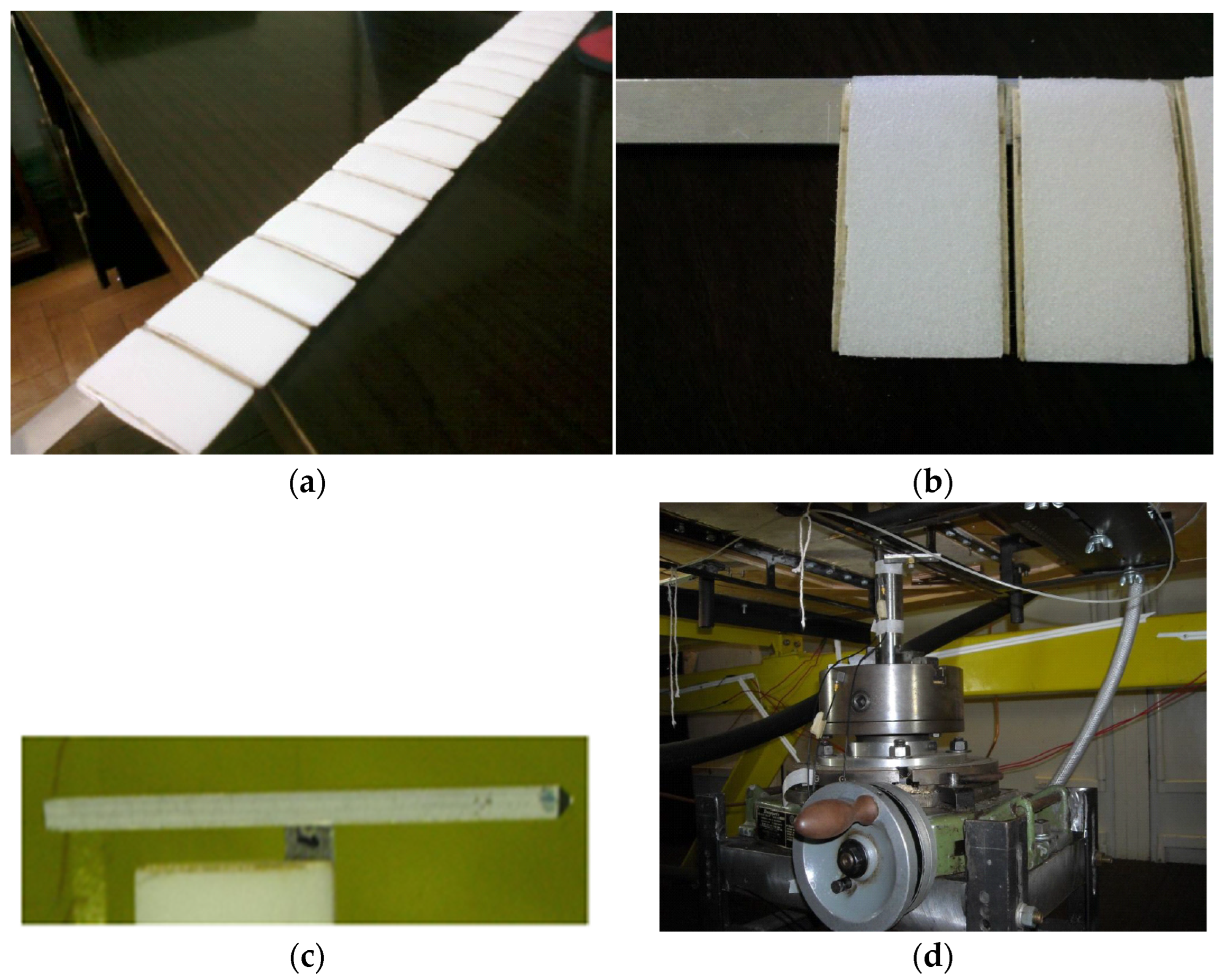
The case study for this paper has its design inspired by [2], dimensioned and built as [13]. The very flexible structure is an aluminum flat plate with a very low width (beam-like structure), and it is covered by a foam responsible for the aerodynamic shape of the NACA 0012 airfoil (Figure 1). All the dimensions presented here are the same as those used in computational experiments. The wind tunnel results presented here are the same as [13]. The model has the following geometric characteristics:

• Airfoil: NACA0012. This information is necessary for dynamic stall models and to obtain general aerodynamic characteristics;
• Dimension: 457 mm × 50 mm (span × chord). These values are also used in the aerodynamic model representation (Peters’ model, Equations (6) and (7));
• Structure dimension: 457 mm × 12.7 mm × 1016 mm (length × width × thickness). These dimensions are used in the strain-based geometrically nonlinear formulation;
• Slender body: 14.4 g (mass), 6.35 mm (squared cross section), 132 mm (length). In the strain-based geometrically nonlinear formulation, it is modeled a concentrated mass at the tip, and this information is necessary to calculate the inertia.

The model is positioned in the wind tunnel section attached to the floor of the wind tunnel. The wind tunnel used in the tests has a rectangular and closed test section with 1 m width and 1.28 m in height, a maximum velocity of 80 m/s, and a power of 200 H, as shown in Figure 2. The air density is considered to be 1.225 kg/m³ for the computational experiments (shall be close to the wind tunnel experiments).

The model is tested only for 0° of the angle of attack, and the accelerometers are positioned close to the wing root. Although the accelerometers’ positions are not ideal and result in noisier data, the model is very flexible and presents large displacement vibration, and the instrumentation cables influence the model behavior. The procedure is the same as presented in [16]:

• First, a linear aeroelastic analysis is computed using commercial software, NASTRAN^®, to generate the modal basis and ZAERO^® to perform the aeroelastic analysis. These results are shown in

  Table 1. Flutter results.

  	Computational Linear	Computational Nonlinear	Experiment
  Velocity [m/s]	22.4	17.2	18.9
  Frequency [Hz]	17.2	15.8	18.0

  ;
• After the design stage, the model is selected to be built and tested (Figure 1). It is a wing model with a NACA0012 symmetric airfoil, a very flexible structure due to its low width and large span, and a slender aluminum body to induce the torsion mode to couple with the second bending mode (their natural frequencies are close enough to coalesce at the flutter speed). It is clamped at the wind tunnel floor;
• A nonlinear flutter analysis is carried out using a framework that considers a beam model subjected to nonlinear geometric deformations and an unsteady aerodynamic model, as presented in Section 2 of this paper.

Table 1 shows that the results from commercial software, represented by the computational linear column, the nonlinear analysis, and the wind tunnel results, are all close to each other [16]. There is an error when the computational nonlinear result is compared to the experiment. This result partially validates the nonlinear framework in terms of velocity and frequency compared to the wind tunnel.

4. Post-Flutter Analysis

After the traditional signal analysis, the 0–1 test is performed as well as the attractor reconstruction using Takens’ theory. With these results, it is possible to determine if the system corresponding to each flow velocity presents periodic or chaotic behavior. There are results for flows below the flutter velocity, at the flutter onset, and for velocities above it.

For all 0–1 test simulations, the parameter c is chosen randomly between 0 and π, and the entire time history is used, considering only after the transient. It is possible to observe the differences in the system’s behavior according to the flow velocity and the dynamic stall correction chosen.

This Section is divided into three: results for velocities before flutter, at flutter, and post flutter, but the experimental results are obtained only for the flutter velocity.

4.1. Results for Velocities before Flutter

The first cases to be investigated here are the computational experiments considering flow velocities before achieving flutter. Here, it will be presented the results for velocities 12 m/s and 15 m/s.

For the 0–1 test, it is possible to verify from Figure 3 that the points are mostly concentrated close to zero despite there being a few at one or close to one. For this reason, it is necessary to calculate the median value of K [25], as proposed in Equation (32).

From Figure 3, it can be observed that a large concentration of points close to zero for 12 m/s, 15 m/s, and only when the Boeing–Vertol dynamic stall correction is applied in the flutter velocity case.

For all velocities below flutter velocity, the auxiliary trajectories (Figure 4) are bounded for all cases, indicating periodic behavior. From

Table 2. 0–1 test results: Computational experiment. Velocities before flutter.

V [m/s]	Without Dynamic Stall Correction	Boeing-Vertol Dynamic Stall Correction	Gangwani Dynamic Stall Correction
12	−0.0345	−0.0376	−0.0492
15	−0.0257	−0.0183	−0.0446

, the results from the 0–1 test are mostly close to zero for velocities below flutter, demonstrating periodic behavior.

The next step is to evaluate this same aeroelastic system using the classical reconstruction based on Takens’ theory and calculate the Lyapunov exponent for the same cases. The attractor reconstruction is important to confirm if the 0–1 test for aeroelastic systems is in good agreement with the wind tunnel results by analyzing the system attractor.

The first step for the attractor reconstruction and the determination of the Lyapunov exponent is to calculate the delay parameter (using mutual average information) and the embedded dimension (using the Cao method). These parameters do not change much by adding a dynamic stall correction, so only one value will be shown for brevity.

For numerical simulations, different wind velocities lower than flutter velocity are used, as shown in

Table 3. Delay parameters and embedded dimension for velocities before flutter.

V [m/s]	Delay Parameter	Embedded Dimension
12	26	2
15	23	2

, and after calculating the values for the embedded dimension and delay parameter, the attractors of the system are reconstructed and presented in Figure 5.

By observing Figure 5, the reconstructed attractors for pre-flutter cases are closed loops in all cases, so limit-cycle oscillations, or LCO (to be confirmed with the Lyapunov exponent, shown in

Table 4. Lyapunov exponent for the computational experiment: before flutter velocity.

V [m/s]	Without Dynamic Stall Correction	Boeing–Vertol Dynamic Stall Correction	Gangwani Dynamic Stall Correction
12	−6.9222	−8.5213	−6.9553
15	−6.1489	−5.4742	−5.7752

).

The Lyapunov exponents are negative, which verifies the reconstruction attractor appearance and the 0–1 test, resulting in periodic behavior or LCO. The further the Lyapunov exponent goes from zero, the more chaotic the system is. The Lyapunov exponent gives the stability of the system. Positive Lyapunov values mean that the system diverges. Negative values mean that the system is stationary or periodically stable, so it is not chaotic, as expected from the 0–1 test and the attractor reconstruction.

4.2. Results for Flutter Velocity

For the flutter velocity, the same analysis is performed, not only for the computational experiments but also for the wind tunnel experiments (since there are experimental data for these cases only). First, the result of the 0–1 test before calculating the median is shown in Figure 6.

At flutter velocity (17.2 m/s), this same conclusion as in Section 4.1 is observed, but only when a Boeing–Vertol correction for dynamic stall is applied. Without dynamic stall correction and when the Gangwani correction is considered, the results are close to one, which demonstrates chaotic behavior. As recommended by [25], the auxiliary trajectories are part of the interpretation of the results calculated in

Table 5. 0–1 test results: Computational experiment.

V [m/s]	Without Dynamic Stall Correction	Boeing–Vertol Dynamic Stall Correction	Gangwani Dynamic Stall Correction
17.2	0.9122	−0.0244	0.9696

and are shown in Figure 7.

For the flutter velocity (17.2 m/s), only when Boeing–Vertol dynamic stall correction is applied is the auxiliary trajectory bounded. Without dynamic stall correction and when the Gangwani correction is applied, the auxiliary trajectory is similar to a Brownian movement, which means that the dynamic behavior of the system is chaotic, according to the methodology.

The delay parameter and embedded dimension for the attractor reconstruction and Lyapunov exponent calculation are given in

Table 6. Delay parameters and embedded dimension.

V [m/s]	Delay Parameter	Embedded Dimension
17.2	28	3

and are shown in Figure 8.

Like expected to occur in the flutter velocity (from 0–1 test), a chaotic attractor is observed except when the Boeing–Vertol correction is applied. A similar result is obtained by the 0–1 test. From

Table 7. Lyapunov exponent for the computational experiment: flutter velocity.

V [m/s]	Without Dynamic Stall Correction	Boeing–Vertol Dynamic Stall Correction	Gangwani Dynamic Stall Correction
17.2	0.3637	−4.9626	1.1936

, there is weak chaos in flutter velocity without dynamic stall correction (although positive, it is a value close to zero, so the orbit does not diverge fast).

The results of the wind tunnel experiments are given next. The same steps are followed with the measured data. First, the 0–1 test is calculated, and the results are given in Figure 9.

For the 0–1 test presented here, the c values are randomly chosen between 0 and π. From Figure 9, the k values are not concentrated close to zero or one, and they look more dispersed than the results in Figure 6. The median value calculated is 0.7815. This result is closer to one than zero, so the tendency is to conclude that this system has chaotic behavior as predicted by computational results without dynamic stall correction or with Gangwani correction for dynamic stall.

To proceed with the attractor reconstruction, the first parameters to be estimated are the delay parameter and the embedded dimension. According to Takens’ theory [26], these values are 22 and 5, respectively.

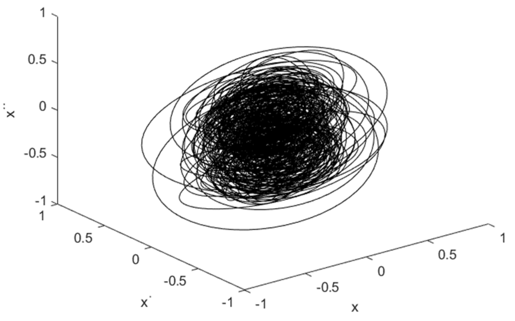
After determining the delay parameter and the embedded dimension and using the acquired time history, the system attractor is reconstructed, as shown in Figure 10.

As observed in Figure 10, this system dynamic might present chaotic behavior. The Lyapunov exponent for this case is 0.3369, which is positive, representing an unstable system’s dynamic. However, it is a low positive number, so it can be concluded that this system presents a weak chaotic behavior, which is in good agreement with the 0–1 test (value close to 0.5). This Lyapunov exponent result is the closest to that obtained when no dynamic stall correction is applied (0.3637), which shall mean either this aeroelastic system did not present dynamic stall during the wind tunnel test or these semi-empirical models are not good enough for chaotic systems. In this case, instead of using a semi-empirical model, it is recommended for future research to apply fluid-structure interaction (FSI) methodology to investigate this high-aspect ratio case further.

Table 5 compares the Lyapunov exponent and the 0–1 test only in flutter velocity (17.2 m/s) for the different cases of dynamic stall.

The results in

Table 8. Lyapunov exponent × 0–1 test for the high-aspect-ratio model.

	Wind Tunnel	Without Correction	Boeing–Vertol	Gangwani
Lyapunov exponent	0.3369	0.3637	−4.9626	1.1936
0–1 Test	0.7815	0.9122	−0.0244	0.9696

show good agreement between the computational experiment and the wind tunnel test result in terms of the characterization of the aeroelastic system. This system presents chaotic behavior, but it is necessary to perform a deeper investigation in wind tunnels for higher velocities. This paper will only present the computational results for velocities post-flutter, as shown in the next Section.

4.3. Results for Velocities Post Flutter

Since the results obtained in Section 4.2 demonstrate that the system presents chaotic behavior, a deeper understanding is important. Here, only computational experiments are shown, and wind tunnel experiments are suggested as a topic for future research.

For the post-flutter analysis, three velocities are considered: 20 m/s, 23 m/s, and 25 m/s. As in the other cases, Figure 11 shows the result of the 0–1 test before the median.

As observed in Figure 11, the points are concentrated close to one.

For post-flutter wind velocities, the auxiliary trajectories indicate chaos, except for 23 m/s with Gangwani dynamic stall correction application and for 25 m/s without dynamic stall correction.

The results shown in Figure 11 and Figure 12 are difficult to conclude in some cases, so, as part of the 0–1 test, the median is calculated for all of them and shown in

Table 9. 0–1 test results: computational experiment.

V [m/s]	Without Dynamic Stall Correction	Boeing-Vertol Dynamic Stall Correction	Gangwani Dynamic Stall Correction
20	0.9854	0.9658	0.9789
23	0.9500	0.9653	0.5986
25	0.8906	0.9749	0.8956

. For all post-flutter velocities, chaotic behavior is also observed, as expected from Figure 11 and Figure 12. Also, as expected, the only exception is when the Gangwani dynamic stall correction is applied in the 23 m/s simulation. For this specific case, the result, 0.5986, is inconclusive [23], so the calculation of the Lyapunov exponent shall help.

After calculating the values for the embedded dimension and delay parameter (

Table 10. Delay parameters and embedded dimension.

V [m/s]	Delay Parameter	Embedded Dimension
20	41	3
23	41	3
25	61	3

), the attractors of the system are reconstructed for each flow velocity and presented in Figure 13.

For post-flutter velocities, all attractors look chaotic (Figure 13). Similar to the result observed in Figure 12, there are some doubts regarding 23 m/s with Gangwani correction for dynamic stall. In this case, the 0–1 test is inconclusive. For 25 m/s without dynamic stall correction, the 0–1 test resulted in chaotic behavior. For both cases, the Lyapunov exponent shall give a conclusion, as can be seen in

Table 11. Lyapunov exponent for the computational experiment: post-flutter velocities.

V [m/s]	Without Dynamic Stall Correction	Boeing–Vertol Dynamic Stall Correction	Gangwani Dynamic Stall Correction
20	1.4191	1.5581	1.6949
23	1.7050	1.5044	−3.7661
25	1.7777	1.6791	1.4330

.

An interesting result that shall be verified in more detail in future research is the 23 m/s with Gangwani dynamic stall correction. So far, it is not possible to draw any conclusions about its dynamic behavior. However, the Lyapunov exponent is negative and not close to zero, so this system is periodic. The best way to verify this is by performing a wind tunnel test for this velocity and comparing it with the experimental result.

The important conclusion from the results obtained by the computational experiments is that the 0–1 test is in good agreement with the Lyapunov exponent and attractor reconstruction for all cases, and it is proved to be a good tool when a nonlinear aeroelastic system is tested in a wind tunnel.

5. Conclusions

A simple aeroelastic system was designed, built, and tested in a wind tunnel. A high-aspect ratio and highly flexible model, with NACA0012 airfoil, aluminum slender body at the tip and attached to the wind tunnel floor [13]. During these tests, the model was not destroyed after achieving a flutter velocity, indicating nonlinear behavior.

In this paper, the wind tunnel results are compared with the computational results obtained by applying strain-based geometrically nonlinear methodology coupled with an unsteady Peters’ aerodynamic model. The wind tunnel test time history is obtained only for the flow velocity equal to the flutter velocity. By using nonlinear simulations, the time histories are obtained for different flow velocities before and after the flutter onset. With the time histories, the 0–1 tests are performed and then compared with the Lyapunov exponents (and attractor reconstruction). In most cases, they agree well and provide an overall understanding of complex system behavior, like the one presented in this paper.

Regarding the dynamic stall corrections, the methodologies presented in this paper are semi-empirical, which is a limitation, and more investigation into this phenomenon is recommended. The closest result in terms of the Lyapunov exponent, when comparing the wind tunnel test and the computational result, is without dynamic stall correction. This result might lead to two possible conclusions: dynamic stall is not happening in these models, or these semi-empirical correction models are not enough, and more powerful methodologies are necessary.

Both computational and wind tunnel experiments presented chaotic behavior, considering no dynamic stall correction. Wind tunnel tests might account for other undesirable inputs, such as noise, wind tunnel wall influence, and free play of attachments, which are not considered in the computational model.

In conclusion, it is recommended to apply the 0–1 test for all simulation time histories precedents of tests (wind tunnel or flight), especially high-risk tests, such as flutter. The advantages of the 0–1 test are the ease of implementation and the speed with which results are obtained, whether the system’s dynamic is chaotic or periodic. By doing this, it is possible to understand in advance the behavior of the system and perform additional analysis to act preventively by adding control, changing or adding a flutter mass, changing gains in the control law, etc. It is important to highlight that low-energy chaos usually does not increase structure failure risk, but it is a point of attention since the presence of chaotic dynamic behavior means high sensitivity to initial conditions. Small steps shall increase the safety of the aircraft.

The main topics recommended for future research are performing wind tunnel tests for each velocity, exploring the post flutter and comparing with the computational experiments, designing a filter for the experimental data since the noise might be polluting the overall result, designing an energy harvesting for post flutter cases, obtaining the bifurcation diagram for both computational and wind tunnel experiments, using a different numerical method of integration to obtain the computational results (simulation with follower forces, for example), and using this same approach focusing in flight mechanics.