Solution of a Half-Space in Generalized Thermoelastic Problem in the Context of Two Models Using the Homotopy Perturbation Method

Abstract

This paper estimated the problem of one-dimensional generalized thermoelastic half-space in medium considering two models: the Lord and Shulman (LS) model and the Dual-Phase-Lag (DPL) model. We assumed that the surface of the half-space was free from traction force and under an exponentially varying external heat source at the boundary with time. The technique of homotopy perturbation has been applied to find the approximate solution for the interactions of thermoelasticity with the applied boundary condition. The effect of a heat source that varies with the time and the free traction force are investigated for the temperature, displacement, and stress. The numerical results obtained are presented graphically to show the influence of the new external parameters. The results obtained illustrate the strong impacts on the displacement, temperature, and stress with the variations in the two models as well as the relaxation time parameter. The results show the agreement between the present results and the previous obtained results of the phenomenon and applicable, especially in biology, acoustics, engineering, and geophysics.

1. Introduction

Lord and Shulman [1] pointed out a generalized dynamical model of thermo-elasticity. Green and Lindsay [2] presented a generalized thermo-elasticity theory with double relaxation time terms and modified both the energy equation and the constitutive equations. Chandrasekharaiah [3] discussed the propagation of waves in a one-dimensional linear model of thermoelasticity with energy dissipation (WED). Dhaliwal and Singh [4] studied dynamic coupled thermoelasticity. Hetnarski and Ignaczak [5] developed other thermoelasticity theories. Abo-Dahab et al. [6] investigated the various variables of rotational, gravitational, and magnetic fields with the presence of relaxation times to understand the phenomenon of primary waves and obtain an explanation of this phenomenon. Roychoudhuri [7] studied one-dimensional wave propagation in a thermoelastic half-space using dual-phase-lag theory. Abouelregal [8] studied the Rayleigh waves in a thermoelastic solid half space using a dual-phase-lag theory. Aboueregal and Abo-Dahab [8] considered a dual-phase model of an elastic body for a non-homogeneous medium under the influence of relaxation times that achieves the best value for an infinite velocity. Bayones et al. [9] developed the effect of magnetic fields of a viscoelastic body in different media and applied these results to geophysics. Mukhopadhyay et al. [10] studied the representation of solutions for the generalized thermo-elasticity theory with three phase lags. Chandrasekharaiah and Srinath [11] illustrated wave propagation in one-dimensional thermoelastic half-space without energy dissipation. Chandrasekharaiah [12] studied the theories of hyperbolic thermoelasticity, for example, extended thermoelasticity and temperature-rate-dependent thermoelasticity. Bayones et al. [13] compared the different relaxation times of a porous medium in the presence of photothermal energy. Yadav and Kumar [14] considered the homotopy approach analysis to interactions of thermoelasticity with boundary conditions, such as an exponentially varying heat source with time and free stress. Rashidi, and Pour [15] investigated the analytic approximate solutions for heat transfer due to a stretching sheet and unsteady boundary layer flow using the homotopy analysis method. Kilany et al. [16] used thermal diffusion and porous media under models of thermoelasticity. Behrouz and Kuppalapalle [17] studied the homotopy analysis technique for a magneto hydrodynamic viscoelastic fluid flow and heat transfer in a channel with a stretching wall. Abo-Dahab et al. [18] used the fractional differential calculations to calculate the different speeds and displacements of the primary and secondary waves with the use of many different influences and variables that these waves are affected by. These variables are the primary stress and the thermal relaxation times. The theory used is the three-phase-lag model. Abd-Alla et al. [19] studied the harmonic wave generation in nonlinear thermoelasticity. Mohyud-Din and Noor [20,21], solving fourth-order boundary value problems to partial differential equations, considered the homotopy perturbation technique. Kilany et al. [22,23] investigated the different comparisons of the elasticity theory in an isotropic medium and the usag of elastic materials with a thermal effect. He [24,25] investigated an approximate solution of nonlinear differential equations with nonlinear convolution products. Abo-Dahab et al. [26] used the homotopy perturbation technique on wave propagation in an isotropic, transversely thermoelastic, two-dimensional plate with gravitational effects. Liao [27] considered the homotopy analysis technique for nonlinear phenomena. A singular two-point boundary value problem’s numerical solution was obtained using the domain decomposition homotopy perturbation approach by Roul [28]. Other authors [29,30,31,32,33] have studied elasticity theories of various kinds of analytical and numerical methods and their impact on modern applied fields. Refs. [33,34,35,36,37,38,39,40,41,42,43,44,45] considered numerical methods to solve heat-related problems.

In this paper, we investigated the one-dimensional half-space problem in generalized thermoelastic material considering two theories: the Lord and Shulman (LS) theory and the dual-phase-lag (DPL) model. The half-space surface is assumed to be traction-free and subjected to a heat source with exponentially varying impact at the boundary with time. The homotopy perturbation technique is applied to obtain the approximate solution to thermoelastic interactions under the applied boundary condition. The effect of the heat source varying with time and free traction force are investigated on displacement, temperature, and stress. In this estimation, we obtained the solutions to wave propagation phenomena considering the homotopy perturbation technique and two thermoelastic models (LS and DPL), comparing results between them. This study does not consider previous results obtained by others. The results obtained agree with the previous investigation of the phenomenon and applicable, especially in biology, acoustics, engineering, and geophysics [7,10,14].

2. The Basic Models Used in the Problem

We used new models in generalized thermoelasticity. The two models depend on thermal relaxation time, so the equation of the Lord–Shulman (LS) model takes this form [1]:

$$\kappa {{\rm T}}_{,ii}=\left(\frac{\partial }{\partial t}+\tau \frac{{\partial }^2}{\partial t^2}\right)\left(\rho \hspace{0.17em}{C}_E{\rm T}+\gamma {{\rm T}}_{0}e\right)$$

(1)

Since it uses another relaxation time that measures more accurately than the first relaxation time when near infinity, the equation to the dual-phase-lag (DPL) model takes this form [43]:

$$\kappa \left(1+{\tau }_{\Theta }\frac{\partial }{\partial t}\right){{\rm T}}_{,ii}=\left(\frac{\partial }{\partial t}+\tau \frac{{\partial }^2}{\partial t^2}\right)\left(\rho \hspace{0.17em}{C}_E{\rm T}+\gamma {{\rm T}}_{0}e\right)$$

(2)

3. Basic Idea for the Technique of Homotopy Perturbation

A general equation of this type is considered as follows:

$$L\left(u\right)=0$$

(3)

We assume a homotopy convex in this form [25]:

$$H\left(u,p\right)=\left(1-p\right)F\left(u\right)+pL\left(u\right)$$

(4)

where $\mathrm{F}\left(\mathrm{u}\right)$ is the functional operator for known solution $u_0$ and can be obtained easily.

It is shown that

$$H\left(u,p\right)=0$$

(5)

We have $H\left(u,0\right)=F\left(u\right)$ and $H\left(u,1\right)=L\left(u\right)$. This shows that $H\left(u,p\right)$ implicitly continuously traces a defined curve from a starting point $H\left(u_0,0\right)$ to a solution $H\left(u,1\right)$. The embedding parameter monotonically increases from zero to unity as the problem considered $F\left(u\right)=0$ deforms continuously to the main problem $L\left(u\right)=0$. The embedding parameter can be taken as an expanding parameter. The HPM considers the parameter of homotopy $p\in \left[0,1\right]$ as an expanding parameter to obtain

$$u={\displaystyle \sum _{i=0}^{\infty }{p}^i}{u}_i=u_0+p{u}_1+p^2{u}_2+\cdots \hspace{0.17em}\hspace{0.17em}$$

(6)

If $p\to 1$, then Equation (6) corresponds to Equation (4) and takes the approximate solution of the form:

$$u=\underset{p\to 1}{\lim }\hspace{0.17em}u={\displaystyle \sum _{i=0}^{\infty }{u}_i}$$

(7)

It is well-known that the series of Equation (7) converges for most cases, and the convergence rate depends on $L\left(u\right)$.

4. Problem Formulation and the Fundamental Equations

The motion equation [4] is:

$${\sigma }_{ij,j}=\rho \frac{{\partial }^2{u}_i}{\partial t^2}$$

(8)

The heat conduction equation [5] is:

$$\kappa \left(1+{\tau }_{\Theta }\frac{\partial }{\partial t}\right){{\rm T}}_{,ii}=\left(\frac{\partial }{\partial t}+\tau \frac{{\partial }^2}{\partial t^2}\right)\left(\rho \hspace{0.17em}{C}_E{\rm T}+\gamma {{\rm T}}_{0}e\right)$$

(9)

The constitutive equations take the following form:

$${\sigma }_{ij}=2\mu e_{ij}+\lambda e_{kk}{\delta }_{ij}-\gamma \left({\rm T}-{{\rm T}}_0\right){\delta }_{ij}$$

(10)

We consider an isotropic homogeneous and half-space thermoelastic medium which fills the region subjected to a heat source varying exponentially with time on the surface x = 0 boundary plane, which is assumed to be free from traction. The fundamental equations will be taken in the context of two models: the Lord and Shulman (LS) model and the dual-phase-lag (DPL) model. The component of displacement is of the form $u_i=\left(u,0,0\right)\hspace{0.17em}\hspace{0.17em}\hspace{0.17em}\hspace{0.17em}\hspace{0.17em}{u}_y=u_z=0$.

From Equations (8)–(10), we obtain

$$\rho \frac{{\partial }^{2}u}{\partial t^2}=\left(\lambda +2\mu \right)\frac{{\partial }^{2}u}{\partial x^2}-\gamma \frac{\partial {\rm T}}{\partial x}$$

(11)

$$\kappa \left(1+{\tau }_{\Theta }\frac{\partial }{\partial t}\right)\frac{{\partial }^2{\rm T}}{\partial x^2}=\left(\frac{\partial }{\partial t}+\tau \frac{{\partial }^2}{\partial t^2}\right)\left(\rho \hspace{0.17em}{C}_E{\rm T}+\gamma {{\rm T}}_{0}e\right)$$

(12)

$${\sigma }_{xx}=\left(\lambda +2\mu \right)\frac{\partial u}{\partial x}-\gamma \left({\rm T}-{{\rm T}}_0\right)$$

(13)

The non-dimensional variables are defined in the following forms:

$$\begin{array}{l}{x}^{\prime }=c_1\eta x,\hspace{0.17em}\hspace{0.17em}\hspace{0.17em}\hspace{0.17em}\hspace{0.17em}\hspace{0.17em}\hspace{0.17em}\hspace{0.17em}\hspace{0.17em}\hspace{0.17em}{u}^{\prime }=c_1\eta u,\hspace{0.17em}\hspace{0.17em}\hspace{0.17em}\hspace{0.17em}\hspace{0.17em}\hspace{0.17em}\hspace{0.17em}\hspace{0.17em}\hspace{0.17em}\hspace{0.17em}\hspace{0.17em}{t}^{\prime }=c_1^2\eta t,\hspace{0.17em}\hspace{0.17em}\hspace{0.17em}\hspace{0.17em}\hspace{0.17em}\hspace{0.17em}\hspace{0.17em}\hspace{0.17em}\hspace{0.17em}\hspace{0.17em}{\tau }^{\prime }=c_1^2\eta \tau ,\hspace{0.17em}\hspace{0.17em}\hspace{0.17em}\hspace{0.17em}\hspace{0.17em}\hspace{0.17em}\hspace{0.17em}\hspace{0.17em}\hspace{0.17em}\hspace{0.17em}\hspace{0.17em}\hspace{0.17em}{{\tau }^{\prime }}_{\Theta }=c_1^2\eta {\tau }_{\Theta },\\ {\theta }^{\prime }=\frac{{\rm T}}{{{\rm T}}_0},\hspace{0.17em}\hspace{0.17em}\hspace{0.17em}\hspace{0.17em}\hspace{0.17em}\hspace{0.17em}\hspace{0.17em}\hspace{0.17em}\hspace{0.17em}\hspace{0.17em}\hspace{0.17em}\hspace{0.17em}\eta =\frac{\rho C_E}{\kappa },\hspace{0.17em}\hspace{0.17em}\hspace{0.17em}\hspace{0.17em}\hspace{0.17em}\hspace{0.17em}\hspace{0.17em}\hspace{0.17em}\hspace{0.17em}\hspace{0.17em}\hspace{0.17em}{{\sigma }^{\prime }}_{xx}=\frac{{\sigma }_{xx}}{\lambda +2\mu },\hspace{0.17em}\hspace{0.17em}\hspace{0.17em}\hspace{0.17em}\hspace{0.17em}\hspace{0.17em}\hspace{0.17em}\hspace{0.17em}\hspace{0.17em}\hspace{0.17em}\hspace{0.17em}\hspace{0.17em}{c}_1^2=\frac{\lambda +2\mu }{\rho }\end{array}$$

By using non-dimensional variables in Equations (11)–(13), we obtain

$$\frac{{\partial }^{2}u}{\partial x^2}-a_1\frac{\partial \theta }{\partial x}=\frac{{\partial }^{2}u}{\partial t^2}$$

(14)

$$\left(1+{\tau }_{\Theta }\frac{\partial }{\partial t}\right)\frac{{\partial }^2\theta }{\partial x^2}=\frac{\partial \theta }{\partial t}+\tau \frac{{\partial }^2\theta }{\partial t^2}+a_2\left[\frac{{\partial }^{2}u}{\partial t\partial x}+\tau \frac{{\partial }^{3}u}{\partial t^2\partial x}\right]$$

(15)

$${\sigma }_{xx}=\frac{\partial u}{\partial x}-a_1\theta$$

(16)

5. Solution under the Homotopy Perturbation Technique

From Equations (14) and (16), we obtain

$$\frac{{\partial }^2{\sigma }_{xx}}{\partial x^2}=\frac{{\partial }^2{\sigma }_{xx}}{\partial t^2}+a_1\frac{{\partial }^2\theta }{\partial t^2}$$

(17)

From Equations (15) and (16), we obtain

$$\frac{{\partial }^2\theta }{\partial x^2}=\left(1+\epsilon \right)\frac{\partial \theta }{\partial t}+\tau \left(1+\epsilon \right)\frac{{\partial }^2\theta }{\partial t^2}-{\tau }_{\Theta }\frac{{\partial }^3\theta }{\partial t\partial x^2}+a_2\left[\frac{\partial {\sigma }_{xx}}{\partial t}+\tau \frac{{\partial }^2{\sigma }_{xx}}{\partial t^2}\right]$$

(18)

The boundary conditions assumed as follows:

$$\theta \left(t,0\right)=e^{-t},\hspace{0.17em}\hspace{0.17em}\hspace{0.17em}\hspace{0.17em}\hspace{0.17em}\hspace{0.17em}\hspace{0.17em}\hspace{0.17em}\hspace{0.17em}\hspace{0.17em}{\sigma }_{xx}\left(t,0\right)=0$$

(19)

According to the homotopy perturbation, we construct the following homotopy [27]:

$$\frac{{\partial }^2{\sigma }_{xx}}{\partial x^2}+p\left[-\frac{{\partial }^2{\sigma }_{xx}}{\partial t^2}-a_1\frac{{\partial }^2\theta }{\partial t^2}\right]=0$$

(20)

$$\frac{{\partial }^2\theta }{\partial x^2}+p\left[-\left(1+\epsilon \right)\frac{\partial \theta }{\partial t}-\tau \left(1+\epsilon \right)\frac{{\partial }^2\theta }{\partial t^2}+{\tau }_{\Theta }\frac{{\partial }^3\theta }{\partial t\partial x^2}-a_2\left(\frac{\partial {\sigma }_{xx}}{\partial t}+\tau \frac{{\partial }^2{\sigma }_{xx}}{\partial t^2}\right)\right]=0$$

(21)

where $p\in \left[0,1\right]$ is the embedding parameter; we use it for expanding the solution in the following form:

$${\sigma }_{xx}\left(x,t\right)={\sigma }_{xx}^0+p{\sigma }_{xx}^1+p^2{\sigma }_{xx}^2+\dots$$

(22)

$$\theta \left(x,t\right)=\theta +p{\theta }^1+p^2{\theta }^2+p^3{\theta }^3+\dots$$

(23)

The approximate solution of the system can be obtained considering $p=1$ in Equations (22) and (23).

Substituting ${\sigma }_{xx}\left(x,t\right)$ and $\theta \left(x,t\right)$ from Equations (22) and (23) to (20) and (21), respectively, we can obtain linear equations in series form.

Here, we can put only the first few linear equations:

$$p^0:\frac{{\partial }^2{\sigma }_{xx}^0}{\partial x^2}=0$$

(24)

$$p^0:\frac{{\partial }^2{\theta }^0}{\partial x^2}=0$$

(25)

$$p^1:\frac{{\partial }^2{\sigma }_{xx}^1}{\partial x^2}=\frac{{\partial }^2{\sigma }_{xx}^0}{\partial t^2}+a_1\frac{{\partial }^2{\theta }^0}{\partial t^2}$$

(26)

$$p^1:\frac{{\partial }^2{\theta }^1}{\partial x^2}=\left(1+\epsilon \right)\frac{\partial {\theta }^0}{\partial t}+\tau \left(1+\epsilon \right)\frac{{\partial }^2{\theta }^0}{\partial t^2}-{\tau }_{\Theta }\frac{{\partial }^3{\theta }^0}{\partial t\partial x^2}+a_2\frac{\partial {\sigma }_{xx}^0}{\partial t}+a_2\tau \frac{{\partial }^2{\sigma }_{xx}^0}{\partial t^2}$$

(27)

$$p^2:\frac{{\partial }^2{\sigma }_{xx}^2}{\partial x^2}=\frac{{\partial }^2{\sigma }_{xx}^1}{\partial t^2}+a_1\frac{{\partial }^2{\theta }^1}{\partial t^2}$$

(28)

$$p^2:\frac{{\partial }^2{\theta }^2}{\partial x^2}=\left(1+\epsilon \right)\frac{\partial {\theta }^1}{\partial t}+\tau \left(1+\epsilon \right)\frac{{\partial }^2{\theta }^1}{\partial t^2}-{\tau }_{\Theta }\frac{{\partial }^3{\theta }^1}{\partial t\partial x^2}+a_2\frac{\partial {\sigma }_{xx}^1}{\partial t}+a_2\tau \frac{{\partial }^2{\sigma }_{xx}^1}{\partial t^2}$$

(29)

The solution of Equations (24) and (25) can be obtained by using the boundary conditions in Equation (19):

$${\sigma }_{xx}^0\left(x,t\right)={\sigma }_{xx}\left(t,0\right)=0,\hspace{0.17em}\hspace{0.17em}\hspace{0.17em}\hspace{0.17em}\hspace{0.17em}\hspace{0.17em}\hspace{0.17em}\hspace{0.17em}\hspace{0.17em}\hspace{0.17em}\hspace{0.17em}\hspace{0.17em}\hspace{0.17em}\hspace{0.17em}\hspace{0.17em}\hspace{0.17em}\hspace{0.17em}\hspace{0.17em}\hspace{0.17em}{\theta }^0\left(x,t\right)=\theta \left(t,0\right)=e^{-t}$$

(30)

From Equations (26) and (27), we can find:

$$\begin{array}{c}{\sigma }_{xx}^1\left(x,t\right)={\displaystyle {\int }_0^x{\displaystyle {\int }_0^x\frac{{\partial }^2{\sigma }_{xx}^0}{\partial t^2}}}dxdx+a_1{\displaystyle {\int }_0^x{\displaystyle {\int }_0^x\frac{{\partial }^2{\theta }^0}{\partial t^2}}}dxdx\\ {\sigma }_{xx}^1=a_1\left(\frac{x^2}{2!}\right)e^{-t}\end{array}$$

(31)

$$\begin{gathered} \begin{array}{l}{\theta }^1\left(x,t\right)={\displaystyle {\int }_0^x{\displaystyle {\int }_0^x\left(1+\epsilon \right)\frac{\partial {\theta }^0}{\partial t}}}dxdx+\tau {\displaystyle {\int }_0^x{\displaystyle {\int }_0^x\left(1+\epsilon \right)\frac{{\partial }^2{\theta }^0}{\partial t^2}}}dxdx+a_2\tau {\displaystyle {\int }_0^x{\displaystyle {\int }_0^x\frac{{\partial }^2{\sigma }_{xx}^0}{\partial t^2}}}dxdx\\ -{\tau }_{\Theta }{\displaystyle {\int }_0^x{\displaystyle {\int }_0^x\frac{{\partial }^3{\theta }^0}{\partial t\partial x^2}}}dxdx\end{array} \\ {\theta }^1\left(x,t\right)=\left(1+\epsilon \right)\left(\tau -1\right)\left(\frac{x^2}{2!}\right)e^{-t} \end{gathered}$$

(32)

Similarly,

$${\sigma }_{xx}^2\left(x,t\right)=a_1\left[\tau \left(1+\epsilon \right)-\epsilon \right]\left(\frac{x^4}{4!}\right)e^{-t}$$

(33)

$${\theta }^2\left(x,t\right)=\left(1-\tau \right)\left[{\left(1+\epsilon \right)}^2-\tau {\left(1+\epsilon \right)}^2-\epsilon \right]\left(\frac{x^4}{4!}\right)e^{-t}+{\tau }_{\Theta }\left(1+\epsilon \right)\left(\tau -1\right)\left(\frac{x^2}{2!}\right)e^{-t}$$

(34)

$$\begin{array}{l}{\sigma }_{xx}^3\left(x,t\right)=a_1\left[\tau \left(1+\epsilon \right)+{\left(1+\epsilon \right)}^2-2\tau {\left(1+\epsilon \right)}^2-\epsilon \left(2-\tau \right)+{\tau }^2{\left(1+\epsilon \right)}^2\right]\left(\frac{x^6}{6!}\right)e^{-t}\\ +a_1\left[{\tau }_{\Theta }\left(1+\epsilon \right)\left(\tau -1\right)\right]\left(\frac{x^4}{4!}\right)e^{-t}\end{array}$$

(35)

$$\begin{array}{l}{\theta }^3\left(x,t\right)=\left\{\begin{array}{l}-\left(1+\epsilon \right)\left(1-\tau \right)\left[{\left(1+\epsilon \right)}^2-\tau {\left(1+\epsilon \right)}^2-\epsilon \right]\\ +\tau \left(1+\epsilon \right)\left(1-\tau \right)\left[{\left(1+\epsilon \right)}^2-\tau {\left(1+\epsilon \right)}^2-\epsilon \right]\\ -a_1{a}_2\left[\tau \left(1+\epsilon \right)-\epsilon \right]+a_1{a}_2\tau \left[\tau \left(1+\epsilon \right)-\epsilon \right]\end{array}\right\}\left(\frac{x^6}{6!}\right)e^{-t}\\ \hspace{0.17em}\hspace{0.17em}\hspace{0.17em}\hspace{0.17em}\hspace{0.17em}\hspace{0.17em}\hspace{0.17em}\hspace{0.17em}\hspace{0.17em}\hspace{0.17em}\hspace{0.17em}\hspace{0.17em}\hspace{0.17em}+\left\{\tau {\left(1+\epsilon \right)}^2\left(\tau -1\right){\tau }_{\Theta }-{\left(1+\epsilon \right)}^2\left(\tau -1\right){\tau }_{\Theta }\right\}\left(\frac{x^4}{4!}\right)e^{-t}\end{array}$$

(36)

Consequently, we have the solution in a series form as follows:

$${\sigma }_{xx}\left(x,t\right)={\displaystyle \sum _{i=0}^3{\sigma }_{xx}^i}\left(x,t\right)=\left[m_1\frac{x^2}{2!}+m_2\frac{x^4}{4!}+m_3\frac{x^6}{6!}\right]e^{-t}$$

(37)

$$\theta \left(x,t\right)={\displaystyle \sum _{i=0}^3{\theta }^i}\left(x,t\right)=\left[1+n_1\frac{x^2}{2!}+n_2\frac{x^4}{4!}+n_3\frac{x^6}{6!}\right]e^{-t}$$

(38)

From Equation (14), we obtain

$$\frac{\partial u}{\partial x}=\left[a_1+\left(a_1{n}_1+m_1\right)\frac{x^2}{2!}+\left(a_1{n}_2+m_2\right)\frac{x^4}{4!}+\left(a_1{n}_3+m_3\right)\frac{x^6}{6!}\right]e^{-t}$$

(39)

Integrating Equation (35) with respect to x, Equation (39) take the form

$$u\left(x,t\right)=\left[a_1\frac{x}{1!}+\left(a_1{n}_1+m_1\right)\frac{x^3}{3!}+\left(a_1{n}_2+m_2\right)\frac{x^5}{5!}+\left(a_1{n}_3+m_3\right)\frac{x^7}{7!}\right]e^{-t}$$

(40)

where

$$\begin{gathered} \begin{array}{l}{m}_1=a_1,\hspace{0.17em}\hspace{0.17em}\hspace{0.17em}\hspace{0.17em}\hspace{0.17em}\hspace{0.17em}\hspace{0.17em}{m}_2=a_1\left[\tau \left(1+\epsilon \right)-\epsilon \right]+a_1\left[{\tau }_{\Theta }\left(1+\epsilon \right)\left(\tau -1\right)\right],\\ m_3=a_1\left[\tau \left(1+\epsilon \right)+{\left(1+\epsilon \right)}^2-2\tau {\left(1+\epsilon \right)}^2-2\epsilon +\tau \epsilon +{\tau }^2{\left(1+\epsilon \right)}^2\right],\end{array} \\ {n}_1=\left(1+\epsilon \right)\left(\tau -1\right)+{\tau }_{\Theta }\left(1+\epsilon \right)\left(\tau -1\right), \\ {n}_2=\left(1-\tau \right)\left[{\left(1+\epsilon \right)}^2-\tau {\left(1+\epsilon \right)}^2-\epsilon \right]+{\left(1+\epsilon \right)}^2{\left(\tau -1\right)}^2{\tau }_{\Theta }, \end{gathered}$$

Concerning the convergence of the method, the figures obtained indicate the validation and convergence of the method used.

6. Numerical Results and Discussion

Copper is the material chosen for the purposes of numerical estimation. The physical constants are given as

$$\begin{array}{l}\lambda =7.76\times {10}^{10}{\mathrm{Nm}}^{-2}, \hspace{0.17em}\mu =3.86\times {10}^{10}\mathrm{Kg}{.\mathrm{m}}^{-1}{\mathrm{S}}^{-2}, \hspace{0.17em}\rho =8954{\mathrm{kgm}}^{-3},\\ {\alpha }_t=1.78\times {10}^{-5}{\mathrm{k}}^{-1}, \hspace{0.17em}\kappa =8886.73{\mathrm{sm}}^{-3}, C_E=383.1, T_0={293}^{\circ }\mathrm{k}\end{array}$$

Figure 1 and Figure 2 illustrate the variations in displacement $u$ at $t=0.2$ under the L-S and DPL models. It obvious that the distribution of $u$ increases with the increasing the space variable $x$ under the L-S theory, but the distribution of $u$ decreases with increasing space variable $x$ under the DPL theory. The effect of thermal relaxation time appears in the Lord–Shulman (LS) model and is evident in the increase at different values of the relaxation time ($\tau =0.8,\hspace{0.17em}\tau =1$, and ${\tau }_{\theta }=0$). However, the effect of thermal relaxation time also appears in the dual-phase-lag (DPL) model and is evident in the decrease at different values of the relaxation time (${\tau }_{\theta }=0.1,\hspace{0.17em}{\tau }_{\theta }=0.7$, and $\tau =0.8$). Figure 3 and Figure 4 display the variations in temperature $\theta$ at $t=0.2$ under the L-S and DPL theories. The temperature distribution $\theta$ decreases gradually and finally reaches zero after travelling a certain distance. We notice the effect of $LS\hspace{0.17em}>DPL$ in all intervals of variable $x$. Figure 5 and Figure 6 explain the variations in stress ${\sigma }_{xx}$ at $t=0.2$ under the L-S and DPL theories. The distribution of stress ${\sigma }_{xx}$ is increased with the increase in space variable $x$ under the L-S theory, but the distribution of $u$ is decreased with increase in the space variable $x$ under the DPL theory. All figures in 2D and 3D follow the boundary conditions of the phenomenon used.

7. Conclusions

From the results obtained above, we can conclude the following:

• The $\tau \hspace{0.17em}\mathrm{and}\hspace{0.17em}{\tau }_{\Theta }$ parameters have a significant effect on all the fields that have a good result due to the new external parameters.
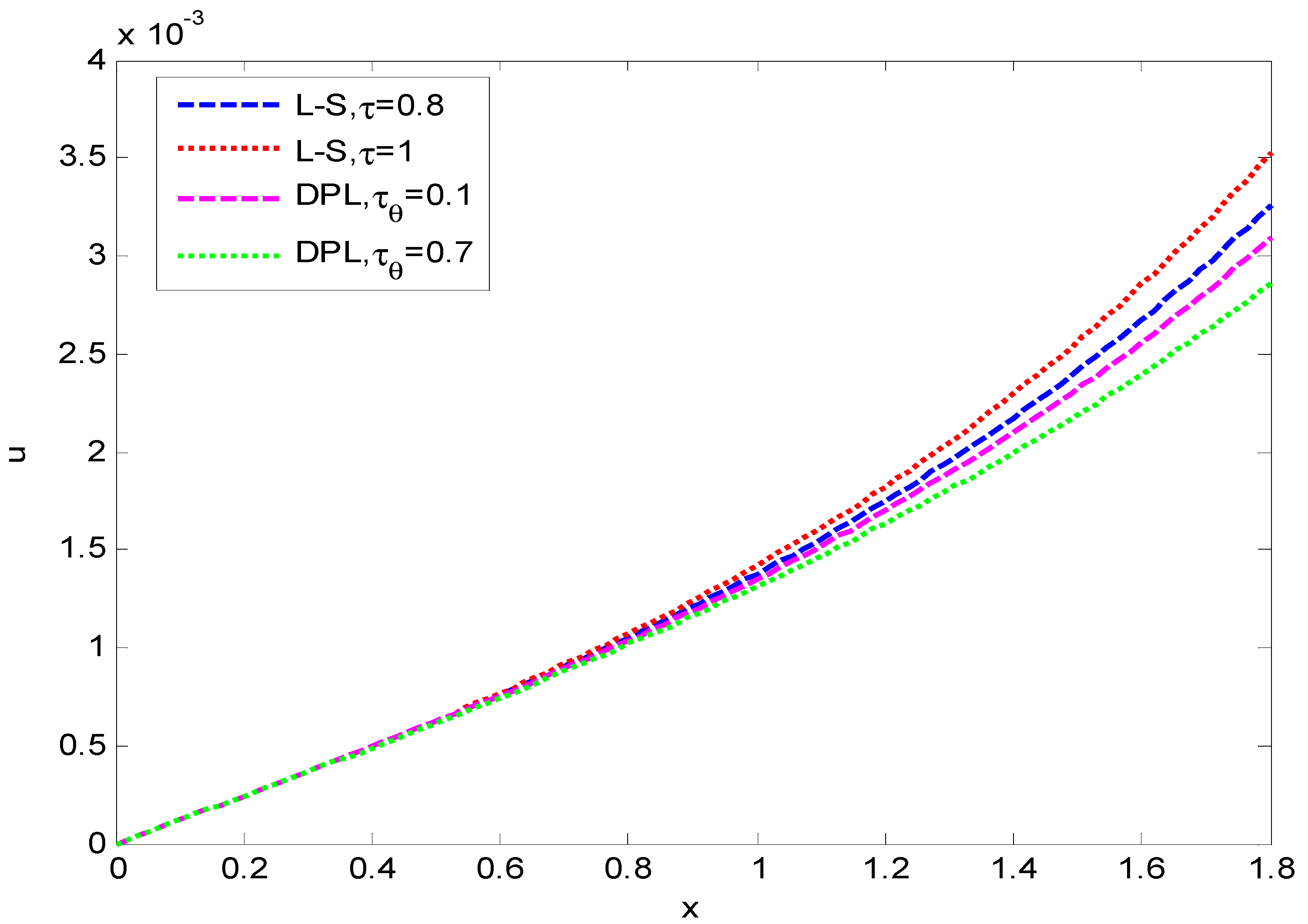
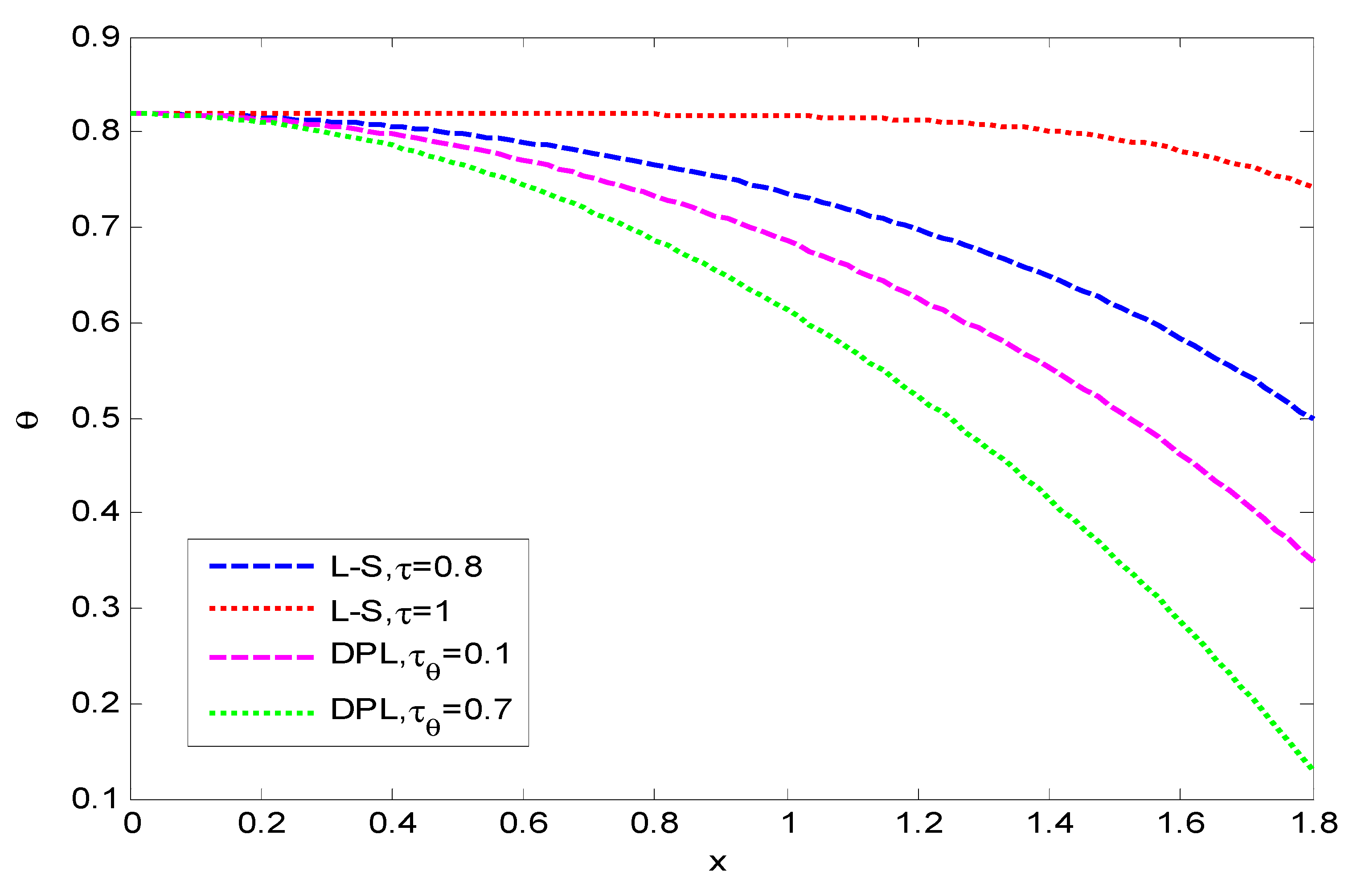
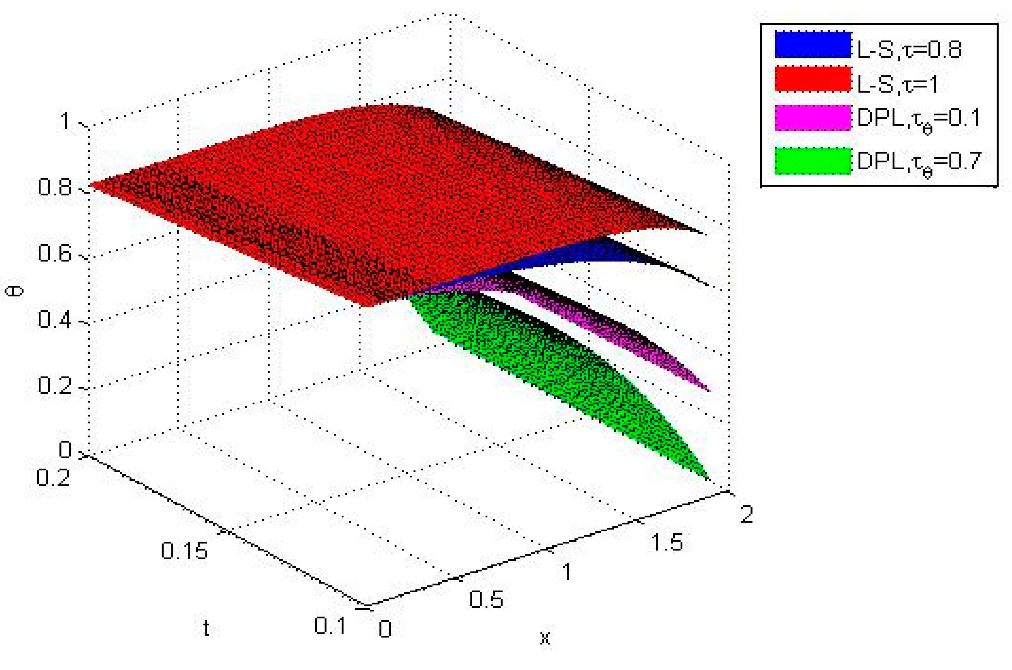
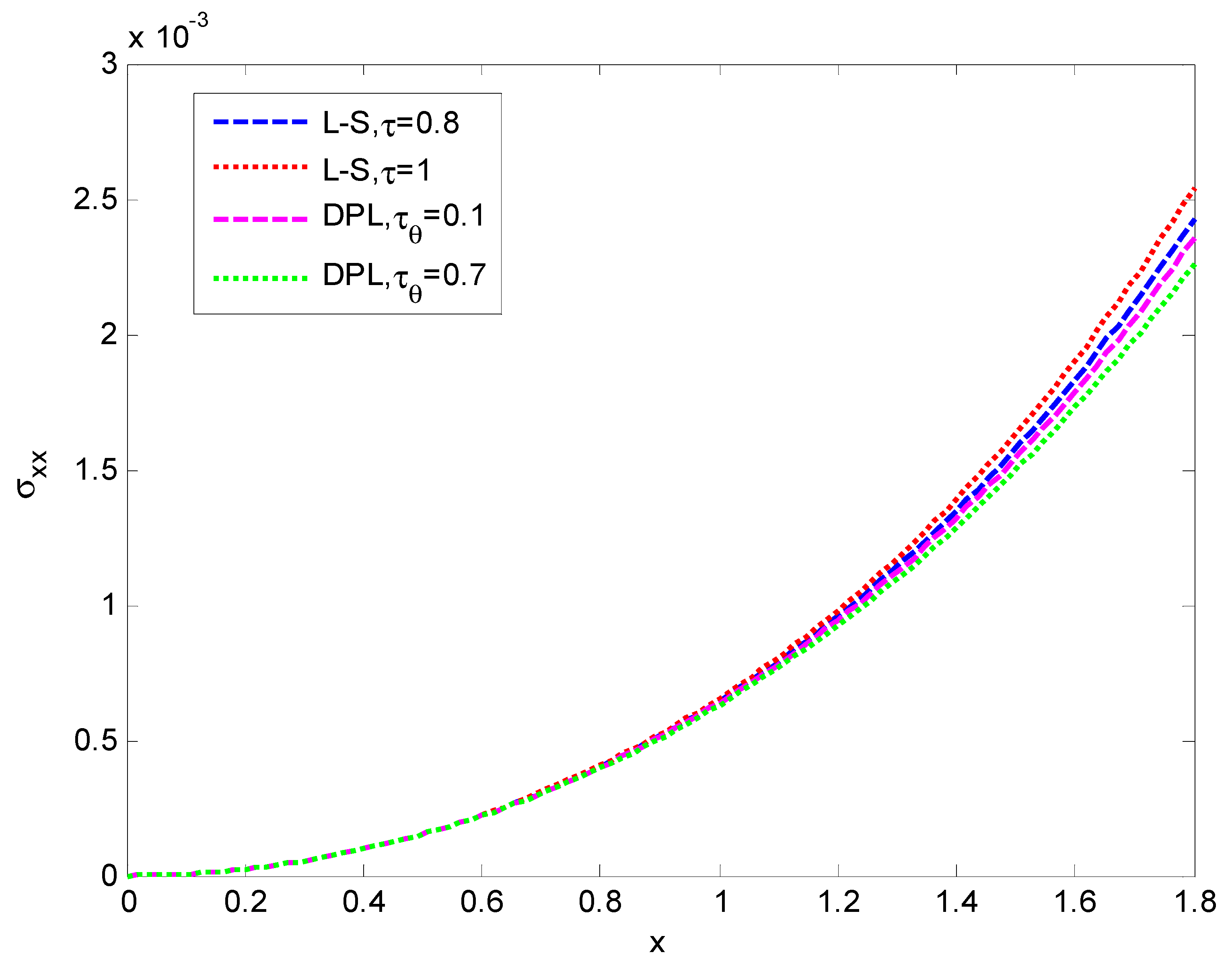
• The comparison of different theories of thermoelasticity, namely the Lord and Shulman (LS) and Chandrasekharaiah and Tzou (DPL) models, is very clear and shows significantly different values between the two theories.
• All boundary conditions satisfy the physical quantities.
• The homotopy perturbation method (HPM) can be used to derive displacement, temperature, and stress analytically.
• The results obtained illustrate the strong impact on the displacement, temperature, and stress with the variations in the two models as well as the relaxation time parameters.
• The results obtained agree with the previous investigation of the phenomenon and are applicable, especially, to biology, acoustics, engineering, and geophysics [7,10,14].

References

1. Lord, H.W.; Shulman, Y. A generalized dynamical theory of thermo elasticity. J. Mech. Phys. Solids 1967, 15, 299–309. [Google Scholar] [CrossRef]
2. Green, A.E.; Lindsay, A. Thermoelasticity. J. Elast. 1972, 2, 1–7. [Google Scholar] [CrossRef]
3. Chandrasekharaiah, D.S. One-dimensional wave propagation in the linear theory of thermoelasticity with energy dissipation. J. Therm. Stress. 1996, 19, 695–710. [Google Scholar] [CrossRef]
4. Dhaliwal, R.S.; Singh, A. Dynamic Coupled Thermoelasticity; Hindustan Publishing Corporation: New Delhi, India, 1980; p. 726. [Google Scholar]
5. Hetnarski, R.B.; Ignaczak, J. Generalized Thermoelasticity. J. Therm. Stress. 1999, 22, 451–476. [Google Scholar]
6. Abo-Dahab, S.M.; Rida, S.Z.; Mohamed, R.A.; Kilany, A.A. Rotation, Initial Stress, Gravity and Electromagnetic Field Effect on P Wave Reflection from Stress-Free Surface Elastic Half-Space with Voids under Three Thermoelastic Models. Mech. Mech. Eng. 2018, 22, 313–328. [Google Scholar] [CrossRef]
7. RoyChoudhuri, S.K. One-dimensional thermoelastic waves in elastic half-space with dual phase-lag effects. J. Mech. Mater. Struct. 2007, 2, 489–503. [Google Scholar] [CrossRef]
8. Abouelregal, A.E. Rayleigh waves in a thermoelastic solid half space using dual-phase-lag model. Int. J. Eng. Sci. 2011, 49, 781–791. [Google Scholar] [CrossRef]
9. Bayones, F.S.; Abo-Dahab, S.M.; Abd-Alla, A.M.; Kilany, A.A. Electromagnetic Field and Three-phase-lag in a Compressed Rotating Isotropic Homogeneous Micropolar Thermo-viscoelastic Half-space. Math. Methods Appl. Sci. 2021, 44, 9944–9965. [Google Scholar] [CrossRef]
10. Mukhopadhyay, S.; Kothari, S.; Kumar, R. On the Representation of Solutions for the Theory of Generalized Thermoelasticity with Three Phase Lags. Acta Mech. 2010, 214, 305–314. [Google Scholar] [CrossRef]
11. Chandrasekharaiah, D.S.; Srinath, K.S. One-dimensional Waves in a Thermoe-lastic Half-Space without Energy Dissipation. Int. J. Eng. Sci. 1996, 34, 1447–1455. [Google Scholar] [CrossRef]
12. Chandrasekharaiah, D.S. Hyperbolic Thermoelasticity: A Review of Recent Literature. Appl. Mech. Rev. 1998, 51, 705–729. [Google Scholar] [CrossRef]
13. Bayones, F.S.; Kilany, A.A.; Abouelregal, A.E.; Abo-Dahab, S.M. A rotational gravitational stressed and voids effect on an electromagnetic photothermal semiconductor medium under three models of thermoelasticity. Mech. Based Des. Struct. Mach. 2021, 51, 1115–1141. [Google Scholar] [CrossRef]
14. Sudhakar, Y.; Kumar, A. A Homotopy Analysis Approach to Thermoelastic In-teractions under the Boundary Condition: Heat Source Varying Exponentially with Time and Zero Stress. Int. J. Sci. Res. 2015, 4, 2126–2129. [Google Scholar]
15. Rashidi, M.M.; Mohimanian Pour, S.A. Analytic approximate solutions for un-steady boundary layer flow and heat transfer due to a stretching sheet by homotopy analysis method. Nonlinear Anal. Model. Control 2010, 15, 83–95. [Google Scholar] [CrossRef]
16. Kilany, A.A.; Abo-Dahab, S.M.; Abd-Alla, A.M.; Abdel-Salam, E.A.-B. Non-integer order analysis of electro-magneto-thermoelastic with diffusion and voids considering Lord–Shulman and dual-phase-lag models with rotation and gravity. Waves Random Complex Media 2022, 1–31. [Google Scholar] [CrossRef]
17. Behrouz, R.; Kuppalapalle, V. Homotopy analysis method for MHD viscoelastic fluid flow and heat transfer in a channel with a stretching wall. Commun. Nonlinear Sci. Numer. Simul. 2012, 17, 4149–4162. [Google Scholar]
18. Abo-Dahab, S.M.; Kilany, A.A.; Abdel-Salam, E.A.-B.; Hatem, A. Fractional derivative order analysis and temperature-dependent properties on p- and SV-waves reflection under initial stress and three-phase-lag model. Results Phys. 2020, 18, 103270. [Google Scholar] [CrossRef]
19. Abd-Alla, A.-E.N.; Ghaleb, A.; Maugin, G. Harmonic wave generation in nonlinear thermoelasticity. Int. J. Eng. Sci. 1994, 32, 1103–1116. [Google Scholar] [CrossRef]
20. Mohyud-Din, S.T.; Noor, M.A. Homotopy perturbation method for solving fourth-order boundary value problems. Math. Probl. Eng. 2007, 2007, 98602. [Google Scholar] [CrossRef]
21. Mohyud-Din, S.T.; Noor, M.A. Homotopy perturbation method for solving partial differential equations. Z. Naturforschung 2009, 64, 157–170. [Google Scholar] [CrossRef]
22. Kilany, A.; Abd-Alla, A.; Abo-Dahab, S.M. On thermoelastic problem based on four theories with the efficiency of the magnetic field and gravity. J. Ocean Eng. Sci. 2022. [Google Scholar] [CrossRef]
23. Kilany, A.A.; Abo-Dahab, S.M.; Abd-Alla, A.M.; Abd-Alla, A.N. Photothermal and void effect of a semiconductor rotational medium based on Lord–Shulman theory. Mech. Based Des. Struct. Mach. 2020, 50, 2555–2568. [Google Scholar] [CrossRef]
24. He, J.H. Approximate solution of nonlinear differential equations with convolution product nonlinearities. Comput. Methods Appl. Mech. Eng. 1998, 167, 69–73. [Google Scholar] [CrossRef]
25. He, J.H. Homotopy perturbation technique. Comput. Methods Appl. Mech. Eng. 1999, 178, 257–262. [Google Scholar] [CrossRef]
26. Abo-Dahab, S.M.; Abd-Alla, A.M.; Kilany, A.A. Homotopy perturbation method on wave propagation in a transversely isotropic thermoelastic two-dimensional plate with gravity field. Numer. Heat Transf. Part A Appl. 2022, 82, 398–410. [Google Scholar] [CrossRef]
27. Liao, S. On the homotopy analysis method for nonlinear problems. Appl. Math. Comput. 2004, 147, 499–513. [Google Scholar] [CrossRef]
28. Roul, P. On the numerical solution of singular two-point boundary value problems: A domain decomposition homotopy perturbation approach. Math. Methods Appl. Sci. 2017, 40, 7396–7409. [Google Scholar] [CrossRef]
29. Pinheiro, I.F.; Sphaier, L.A.; Alves, L.S.d.B. Integral transform solution of integro-differential equations in conduction-radiation problems. Numer. Heat Transf. Part A Appl. 2018, 73, 94–114. [Google Scholar] [CrossRef]
30. Philipbar, B.M.; Waters, J.; Carrington, D.B. A finite element Menter Shear Stress turbulence transport model. Numer. Heat Transf. Part A Appl. 2020, 77, 981–997. [Google Scholar] [CrossRef]
31. Abd-Alla, A.M.; Abo-Dahab, S.M.; Kilany, A.A. Finite difference technique to solve a problem of generalized thermoelasticity on an annular cylinder under the effect of rotation. Numer. Methods Partial. Differ. Equ. 2021, 37, 2634–2646. [Google Scholar] [CrossRef]
32. Abdelhady, M.; Wood, D. Effect of thermal boundary condition on forced convection from circular cylinders. Numer. Heat Transf. Part A Appl. 2019, 76, 420–437. [Google Scholar] [CrossRef]
33. Ahmad, F.; Gul, T.; Khan, I.; Saeed, A.; Selim, M.M.; Kumam, P.; Ali, I. MHD thin film flow of the Oldroyd-B fluid together with bioconvection and activationn energy. Case Stud. Therm. Eng. 2021, 27, 101218. [Google Scholar] [CrossRef]
34. Dawar, A.; Islam, S.; Shah, Z.; Lone, S.A. A comparative analysis of the magnetized sodium alginate-based hybrid nanofluid flows through cone, wedge, and plate. ZAMM 2022, 103, e202200128. [Google Scholar] [CrossRef]
35. Sedelnikov, A.; Serdakova, V.; Orlov, D.; Nikolaeva, A. Investigating the temperature shock of a plate in the framework of a static two-dimensional formulation of the thermoelasticity problem. Aerospace 2023, 10, 445. [Google Scholar] [CrossRef]
36. Antaki, P.J. Effect of dual-phase-lag heat conduction on ignition of a solid. J. Thermophys. Heat Transf. 2000, 14, 276–278. [Google Scholar] [CrossRef]
37. Marin, M. Cesaro means in thermoelasticity of dipolar bodies. Acta Mech. 1997, 122, 155–168. [Google Scholar] [CrossRef]
38. Marin, M.; Ellahi, R.; Chirilă, A. On solutions of Saint-Venant’s problem for elastic dipolar bodies with voids. Carpathian J. Math. 2017, 33, 219–232. [Google Scholar] [CrossRef]
39. Marin, M.; Nicaise, S. Existence and stability results for thermoelastic dipolar bodies with double porosity. Contin. Mech. Thermodyn. 2016, 28, 1645–1657. [Google Scholar] [CrossRef]
40. Watts, H.A. Step size control in ordinary differential equation solvers. Trans. Soc. Comput. Simul. 1984, 1, 15–25. [Google Scholar]
41. Loud, W.S. On the long-run error in the numerical solution of certain differential equations. J. Math. Phys. 1949, 28, 45–49. [Google Scholar] [CrossRef]
42. Hammer, P.C.; Hollingsworth, J.W. Trapezoidal methods of approximating solutions of deferential equations. MTAC 1955, 9, 92–96. [Google Scholar]
43. Lin, W. Global existence theory and chaos control of fractional differential equations. J. Math. Anal. Appl. 2007, 332, 709–726. [Google Scholar] [CrossRef]
44. Kanth, A.R.; Aruna, K. Two-Dimensional Differential Transform Method for Solving Linear and Non-Linear Schrödinger Equation. Chaos Solitons Fractals 2009, 41, 2277–2281. [Google Scholar] [CrossRef]
45. Singh, J.; Kumar, D.; Rathore, S. Application of Homotopy Perturbation Transform Method for Solving Linear and Nonlinear Klein-Gordon Equations. Inf. Comput. 2012, 7, 131–139. [Google Scholar]
Figure 1. Displacement variation in u at t = 0.2 under L-S and DPL theories.
Axioms 12 00827 g001
Figure 2. Three-dimensional variation in displacement u under L-S and DPL theories.
Axioms 12 00827 g002
Figure 3. Temperature variation in θ at t = 0.2 under L-S and DPL theories.
Axioms 12 00827 g003
Figure 4. Three-dimensional variation in temperature θ under L-S and DPL theories.
Axioms 12 00827 g004
Figure 5. Stress variation in σ x x at t = 0.2 under L-S and DPL theories.
Axioms 12 00827 g005
Figure 6. Three-dimensional variation in stress σ x x under L-S and DPL theories.
Axioms 12 00827 g006
Disclaimer/Publisher’s Note: The statements, opinions and data contained in all publications are solely those of the individual author(s) and contributor(s) and not of MDPI and/or the editor(s). MDPI and/or the editor(s) disclaim responsibility for any injury to people or property resulting from any ideas, methods, instructions or products referred to in the content.