Designing a Secure Mechanism for Image Transferring System Based on Uncertain Fractional Order Chaotic Systems and NLFPID Sliding Mode Controller

Abstract

A control method for the robust synchronization of a class of chaotic systems with unknown time delay, unknown uncertainty, and unknown disturbance is presented. The robust controller was designed using a nonlinear fractional order PID sliding surface. The Lyapunov method was used to determine the update laws, prove the stability of the proposed mechanism, and guarantee the convergence of the synchronization errors to zero. The simulation was performed using MATLAB software to evaluate the performance of the proposed mechanism, and the results showed that it was efficient. Finally, the proposed method was combined with a secure communication application to encrypt images, and the results obtained were favorable regarding the standard criteria of correlation, NPCR, PSNR, and information entropy.

1. Introduction

Chaos is a nonlinear phenomenon that appears to be random but actually follows a pattern. It was discovered about a half-century ago by Lorenz [1]. Scientists began to pay more attention to the phenomenon of chaos after that. Some systems, including the Liu system [2], the IU system [3], and the Chen system [4], have been proposed on the basis of Lorenz’s ideas. About 300 years ago, fractional calculations were introduced, and more complete definitions and theorems have been introduced since then [5]. Physical systems can be represented as integer or fractional equations in this context. It is evident that modeling using fractional order systems can have more accuracy than modeling with integer order systems. Recently, the description of systems using fractional calculus has been developed in various sciences, including chemical reaction systems [6,7], biological systems [8,9], power converters [10], electrochemical processes [11], robotics [12], and others. The problem of synchronizing two chaotic systems has piqued the interest of scientists working in the field of secure communication over the past two decades. In fact, the synchronization of two chaotic systems can be described as a situation in which two or more chaotic systems coordinate their responses by the controller. As a result, two subsystems, the main or driving system and the slave or response system, constitute a coupled system. The master system’s response is unconstrained and drives the slave system.

To tackle the problem, Petras et al. presented a fractional sliding surface [13]. Zare Hallaji et al. [14,15] presented research on the synchronization of positive and fractional chaotic systems with system uncertainty. They evaluated the conditions of the described problem from several perspectives, including unknown uncertainties in the system characteristics, in their research. In [16], the chaotic system was synchronized using a nonlinear observer and the benefit of adaptive control in order to determine the system’s uncertainties. In this design, a sliding surface equivalent to one of the system states was provided, and its stability was demonstrated using a Lyapunov function. The authors of [17] proposed an adaptive terminal sliding mode controller (ATSMC). First, a fractional order sliding surface for the master and slave system was introduced in this article. The stability of the suggested controller was then examined, as was the ongoing convergence of the error in the synchronization problem.

A sliding surface based on the nonlinear fractional order PID was developed in this study for the synchronization of two systems with uncertainty and unknown disturbances with unknown and time-varying time delay. The following benefits might be highlighted in this research, which was conducted to synchronize two systems:

-

The use of the nonlinear fractional PID (NLFOPID) sliding surface instead of typical sliding surfaces.

-

The presence of unknown time delays

-

The presence of uncertainty and disturbance with unknown boundaries. Then, using the suitable Lyapunov function and update laws, a control signal was extracted that could be used to overcome the chattering problem by properly adjusting the controller parameters. This is a critical issue for the suggested controller’s implementation. In [10,18], a controller for the synchronization of chaotic systems in finite time was constructed utilizing a sliding surface, and the synchronization of the integer order chaotic system was investigated in [19].

The preliminary calculations of deficit accounts are reported in Section 2 of this article. Section 3 presents the equations characterizing the system as well as the set limitations for uncertainty. Section 4 introduces the sliding surface based on the proportional–integral–nonlinear fractional derivative, as well as the controller architecture. Section 5 investigates the adaptive controller’s stability analysis and update laws. Section 6 presents the simulation results and visualization of the synchronized system. Section 7 discusses chaotic masking for image encryption. Finally, in the last section, conclusions and recommendations are offered.

2. Preliminary Definitions of Fractional Order Differentiation

Definition 1. 

The fractional order integration and differentiation are defined as follows [20]:

$$D_t^q=\left\{\begin{array}{l}\frac{d^q}{d{t}^q}\hspace{1em}\hspace{1em}\hspace{1em}\hspace{1em}q>0\\ 1\hspace{1em}\hspace{1em}\hspace{1em}\hspace{1em}q=0\\ {\int }_q^t(d\tau {)}^{-q}\hspace{1em}\hspace{1em}q<0\end{array}\right.$$

(1)

in which q is a real number.

Definition 2. 

The Riemann–Liouville fractional integral of order q of the function f(t) is defined as follows [21]:

$$t_0{I}_t^{q}f(t)=\frac{1}{\Gamma \left(q\right)}{\int }_{t_0}^t\frac{f\left(\tau \right)}{(t-\tau {)}^{1-q}}d\tau$$

(2)

in which t₀ is the initial time and $\Gamma \left(q\right)$ is the Gamma function defined as follows:

Definition 3. 

Suppose $n-1<q\le n, n\in N$. The fractional Riemann–Liouville differentiation of order q is defined for the function f(t) below [21]:

$$t_0{D}_t^{q}f(t)=\frac{d^{q}f\left(t\right)}{d{t}^q}=\frac{1}{\Gamma (n-q)}\frac{d^n}{d{t}^n}{\int }_{t_0}^t\frac{f\left(\tau \right)}{(t-\tau {)}^{q-n+1}}d\tau$$

(3)

Note 1: In Equation (4), the Riemann-Liouville fractional order integral is first calculated, and then differentiation is performed; thus, the derivative of a constant number in this formulation is not equal to zero.

Definition 4. 

In the continuous function f(t), the Caputo fractional order derivative of order q is defined as follows [21]:

$$t_0{D}_t^{q}f(t)=\left\{\begin{array}{cc}\frac{1}{\Gamma (m-q)}{\int }_{t_0}^t\frac{f^{\left(m\right)}\left(\tau \right)}{(t-\tau {)}^{q-m+1}}d\tau & m-1<q<m\\ \frac{d^{m}f\left(t\right)}{d{t}^m} & q=m\end{array}\right.$$

(4)

$$\Gamma (q)={\int }_0^{\infty }{e}^{-t}{t}^{q-1}dt$$

(5)

Such that m is the first integer number after q.

Lemma 1. 

If f(t) is a constant function and q > 0, the Caputo derivative in Equation (5) for f(t) would be as follows:

$$D^{q}f\left(t\right)=0$$

(6)

The authors of [22] presented the stability analysis of fractional order systems using the direct Lyapunov method, as well as the determination of the necessary and sufficient conditions guaranteeing stability using the Mittag–Leffler concept, and the authors of [23] reviewed the stability analysis of nonlinear systems using convex Lyapunov functions.

Lemma 2 

[23]. Suppose that $h\left(t\right)\in R$ is a continuous and differentiable function. Then, for ${t\ge t}_0$, Equation (7) is satisfied.

$$D^q{h}^2(t)\le 2h(t)\cdot D^{q}h(t)$$

(7)

Lemma 3 

[23]. Suppose that $h\left(t\right)\in R^n$ is a continuous and differentiable function. Then, for ${t\ge t}_0$ , we have:

$$D^q{h}^T(t)·h(t)\le 2h^T(t)\cdot D^{q}h(t)$$

(8)

Theorem 1 

[22]. Assume that the origin $(x=0)$ is the equilibrium point of the fractional order system (5) and that its definition domain covers the origin. Furthermore, $v\left(x\left(t\right),t\right)$ is a continuous and differentiable Lipschitz function, implying the following:

$$\begin{array}{l}{D}^{q}x\left(t\right)=f\left(x,t\right)\\ a_1\parallel x{\parallel }^a\le v\left(x\left(t\right),t\right)\le a_2\parallel x{\parallel }^{ab}\\ D^{q}v\left(x\right(t),t)\le -a_3\parallel x{\parallel }^{ab}\end{array}$$

(9)

in which $0<q<1$ and $a$, $a_1$, $a_2$, $a_3$, $b$ are positive arbitrary constants. Then, the origin is stable in the Mittag–Leffler sense.

Definition 5. 

The continuous function $p:[0,\infty )\to [0,\infty )$ belongs to class k if its derivative is positive and $p\left(0\right)=0$.

Theorem 2 

[22]. Assume $x=0$ is the equilibrium point of the fractional order system (5), the Lipschitz condition for $f\left(x,t\right)$ is satisfied, and $q\in \left(\mathrm{0,1}\right)$. If Equations (8) and (9) are satisfied for the Lyapunov function $v\left(x\left(t\right),t\right)$ and functions ${\delta }_i$ of class K:

$$\begin{array}{l}{\delta }_1\left(\parallel x\parallel \right)\le v\left(x\left(t\right),t\right)\le {\delta }_2\left(\parallel x\parallel \right)\\ D^{q}v\left(x\left(t\right),t\right)\le -{\delta }_3\left(\parallel x\parallel \right) \end{array}$$

(10)

Then, system (5) is asymptotically stable in the Mittag–Leffler sense.

Theorem 3 

[24]. For the fractional order system (5) and the Lyapunov function $v\left(x\right)$, we have:

$$D^{q}v\left(x\right)\le {\left(\frac{\partial v}{\partial x}\right)}^T·D^{q}x={\left(\frac{\partial v}{\partial x}\right)}^T·f(x,t)$$

(11)

Definition 6 

[25]. A continuous piecewise function $f\left(x,t\right)$ has the Lipschitz condition if:

$$‖f\left(x,t\right)-f\left(z,t\right)‖\le {\gamma }_f‖x-z‖, \forall x,z\in R^n$$

(12)

3. System Descriptor Equations

The equations characterizing a class of master–slave chaotic systems with uncertainty and indeterminate time delay in the presence of an unknown disturbance are introduced in this section. Following standardization, the master system dynamics in canonical form are as follows:

$$\left\{\begin{array}{c}{D}^q{x}_i=x_{i+1} 1\le i\le n-1 \\ D^q{x}_n={\sigma }_0^{T}x+f\left(x\left(t-{\tau }_1\right),t\right)+∆f\left(x\left(t\right),t\right)+d_1\left(t\right).\end{array}\right.$$

(13)

The slave system equations are as follows:

$$\left\{\begin{array}{c}{D}^q{y}_i=y_{i+1} 1\le i\le n-1 \\ D^q{y}_n={\sigma }_0^{T}y+g\left(y\left(t-{\tau }_2\right),t\right)+∆g\left(y\left(t\right),t\right)+d_2\left(t\right)+u\left(t\right).\end{array}\right.$$

(14)

The differential equations are written in the forms of well-known chaotic systems, such as the Van der Pol Oscillator, Duffing’s Oscillator, the Genesio–Tesi System, Arneodo’s System, and so on [26], where $x\left(t\right),y\left(t\right)\in R^n$ denote the dynamic states of the master and slave systems, ${\sigma }_0^T$ denotes the constant coefficients in the system’s linear states, and $f\left(x\left(t-{\tau }_1\right),t\right),g\left(y\left(t-{\tau }_2\right),t\right)\in R$ are nonlinear functions with an unknown delay with ${\tau }_1,{\tau }_2$ delays, and $∆f\left(x\left(t\right),t\right),∆g\left(x\left(t\right),t\right)$ represent bounded uncertainty in the master and slave systems. Furthermore, $d_1\left(t\right),d_2\left(t\right)$ indicate the external distortions applied to the master and slave systems, respectively, while $u\left(t\right)$ is the control law applied to the slave system.

Definition 7. 

If the following conditions are satisfied for the systems described in Equations (13) and (14) for all the conditions governing the system, including all initial conditions, uncertainties, unknown time delay, and external disturbance, the system has robust synchronization:

$$\underset{t\to \infty }{\mathit{lim}}\left|y_i\left(t\right)-x_i\left(t\right)\right|=\underset{t\to \infty }{lim}\left|e_i\left(t\right)\right|=0, i=1,\dots ,n.$$

(15)

As a result, $e_i\left(t\right)$ introduces the synchronization error of the master and slave systems.

As a result, the following are the dynamic equations describing the synchronization error for the uncertain chaotic master and slave systems with unknown time delay described in (13) and (14):

$$\left\{\begin{array}{c}{D}^q{e}_i=e_{i+1} 1\le i\le n-1 \\ D^q{e}_n={\sigma }_0^T\left(\mathrm{y}-\mathrm{x}\right)+g\left(y\left(t-{\tau }_2\right),t\right)+∆g\left(x\left(t\right),t\right)+d_2\left(t\right)\\ -\left(f\left(x\left(t-{\tau }_1\right),t\right)+∆f\left(x\left(t\right),t\right)+d_1\left(t\right)\right)+u\left(t\right).\end{array}\right.$$

(16)

Assumption 1. 

The uncertain external disturbances ${\mathit{d}}_{\mathbf{1}}\left(\mathit{t}\right).{\mathit{d}}_{\mathbf{2}}\left(\mathit{t}\right)$ and the uncertain bounded nonlinear uncertainties $∆\mathit{f}\left(\mathit{x}\left(\mathit{t}\right).\mathit{t}\right)$ and $∆\mathit{g}\left(\mathit{x}\left(\mathit{t}\right).\mathit{t}\right)$ in the master and slave systems (13) and (14) meet the following conditions:

$$\begin{array}{l}‖∆\mathit{f}\left(\mathit{x}\left(\mathit{t}\right),\mathit{t}\right)‖\le {\mathit{\beta }}_{\mathbf{1}}{\mathit{\omega }}_{\mathbf{1}}\left(\mathit{x}\right)\\ ‖∆\mathit{g}\left(\mathit{y}\left(\mathit{t}\right),\mathit{t}\right)‖\le {\mathit{\beta }}_{\mathbf{2}}{\mathit{\omega }}_{\mathbf{2}}\left(\mathit{y}\right)\\ ‖{\mathit{d}}_{\mathbf{1}}\left(\mathit{t}\right)‖\le {\mathit{\rho }}_{\mathbf{1}}\\ ‖{\mathit{d}}_{\mathbf{2}}\left(\mathit{t}\right)‖\le {\mathit{\rho }}_{\mathbf{2}}\\ {{\underset{\_}{\mathbf{\tau }}}_{\mathbf{i}}<\mathbf{\tau }}_{\mathbf{i}}<{\overline{\mathbf{\tau }}}_{\mathbf{i}}\end{array}$$

(17)

Such that $‖.‖$ denotes the l₁ norm, ${\beta }_2, {\beta }_1,{\rho }_2,{\rho }_1$ are unknown positive real numbers, and ${\omega }_2\left(·\right),{\omega }_1\left(·\right)$ are positive and known functions. Also, ${\rho }_i<{\overline{\rho }}_i$, ${\beta }_i<{\overline{\beta }}_i$ where ${\overline{\rho }}_i$, ${\overline{\beta }}_i$, ${\overline{\tau }}_i$, and ${\underset{\_}{\tau }}_i$ are known values.

Assumption 2. 

The nonlinear functions $f\left(x\left(t-{\tau }_1\right),t\right), g\left(y\left(t-{\tau }_2\right),t\right)\in R$ satisfy the Lipschitz conditions for any $x\left(t\right),y\left(t\right)\in R$:

$$\begin{array}{l}\left|f\left(x\left(t-{\tau }_1\right)\right)-f\left(x\left(t-{\widehat{\tau }}_1\right)\right)\right|\le l_1\left|{\tau }_1-{\widehat{\tau }}_1\right|=l_1\left|{\tilde{\tau }}_1\right|\\ \left|g\left(y\left(t-{\tau }_2\right)\right)-g\left(y\left(t-{\widehat{\tau }}_2\right)\right)\right|\le l_2\left|{\tau }_2-{\widehat{\tau }}_2\right|=l_2\left|{\tilde{\tau }}_2\right|\end{array}$$

(18)

Table 1. Symbols and concepts.

Symbol	Concept	Symbol	Concept
${\rho }_i$	Disturbance bound	${\widehat{\rho }}_i$	Disturbance bound estimate
${\beta }_i$	Uncertainty bound	${\widehat{\beta }}_i$	Uncertainty bound estimate
$l_i$	Lipschitz constant	${\widehat{\tau }}_i$	Time delay bound estimate
${\tau }_i$	Time delay	${\tilde{\rho }}_i$	Disturbance bound estimate error
${\overline{\rho }}_i$	Disturbance upper bound	${\tilde{\beta }}_i$	Uncertainty bound estimate error
${\overline{\beta }}_i$	Uncertainty upper bound	${\tilde{\tau }}_i$	Time delay estimate error
${\overline{\tau }}_i$	Time delay upper bound	$b$	Positive constant number
${\underset{\_}{\tau }}_i$	Time delay lower bound	$\overline{ϵ}$	Small positive constant number

presents the system parameters and the proposed mechanism:

In this study, all states of the system were directed to and kept on the sliding surface by designing a robust adaptive controller and introducing an integral proportional sliding surface and a fractional order nonlinear derivative. Furthermore, the system’s uncertainties and unknown parameters should be estimated and updated. Then, in the robust synchronization of chaotic systems (13) and (14) in the presence of external distortions, bounded nonlinear uncertainties, and uncertain time delays, the dynamics of the slave system state must match the behavior of the master system dynamics, and the estimation error of the unknown parameters in both chaotic systems approach zero in any circumstance, ensuring the system’s robust stability.

4. The Sliding Mode Control Approach Based on Fractional Order Nonlinear PID Controllers

A proportional integral sliding surface and a nonlinear fractional order derivative are presented in this section in order to synchronize chaotic systems (13) and (14) with unknown uncertainty and unknown time delay. The fractional order sliding surface is as follows, according to the nonlinear fractional order PID controller structure presented in [26], which enhances tracking:

$$s\left(t\right)=h\left(e\right)·\left[k_p{e}_n\left(t\right)+T_I{D}^{-\lambda }{\sum }_{i=1}^n{k}_{1i}{e}_i+T_d{D}^{\delta }{\sum }_{i=1}^n{k}_{2i}{e}_i(t)\right]$$

(19)

Such that $h\left(e\right)$ is a nonlinear function, defined as follows:

$$h\left(e\right)=k_0+\left(1-k_0\right)‖E\left(t\right)‖, k_0\in \left(\mathrm{0,1}\right)$$

(20)

where $‖E\left(t\right)‖=\sum _{i=1}^n\left|e_i\right|$. Coefficients $T_I$ and $T_d$ are time constants of integral and derivative sentences. The parameters $k_{1i}$ and $k_{2i}$ are positive constant values of the sliding surface such that they satisfy the stability of the desired system. If the system is in sliding mode, the following conditions must be met:

$$s\left(t\right)=0, D^{q}s\left(t\right)=0$$

(21)

The fractional order derivative of the sliding surface in Equation (21) is as follows:

$$\begin{array}{l}{D}^{q}s\left(t\right)=(k_0{k}_p{D}^q{e}_n\left(t\right)+k_0{T}_i{D}^{q-\lambda }{\sum }_{i=1}^n{k}_{1i}{e}_i\left(t\right)+k_0{T}_d{D}^{q+\delta }{\sum }_{i=1}^n{k}_{2i}{e}_i\left(t\right)+\left(1-k_0\right)k_p{D}^q\left(‖E\left(t\right)‖e_n\left(t\right)\right)\\ \hspace{1em}\hspace{1em}\hspace{1em}\hspace{1em}\hspace{1em}\hspace{1em}+\left(1-k_0\right)T_I{D}^q\left(‖E\left(t\right)‖D^{-\lambda }{\sum }_{i=1}^n{k}_{1i}{e}_i\left(t\right)\right)+\left(1-k_0\right)T_d{D}^q\left(‖E\left(t\right)‖D^{\delta }{\sum }_{i=1}^n{k}_{2i}{e}_i\left(t\right)\right))=0\end{array}$$

(22)

Now, $D^q{e}_n$ is substituted into Equation (21) using Equation (16):

$$\begin{array}{ll}{D}^{q}s\left(t\right)=& \left(k_0{k}_p\right(g\left(y\left(t-{\tau }_2\right),t\right)+∆g\left(x\left(t\right),t\right)+d_2\left(t\right)-\left(f\left(x\left(t-{\tau }_1\right),t\right)+∆f\left(x\left(t\right),t\right)+d_1\left(t\right)\right)+{\sigma }_0^T·E\left(t\right)\\ & \hspace{1em}\hspace{1em}+u\left(t\right))+k_0{T}_i{D}^{1-\lambda }{\sum }_{i=1}^n{k}_{1i}{e}_i(t)+k_0{T}_d{D}^{1+\delta }{\sum }_{i=1}^n{k}_{2i}{e}_i(t)+\left(1-k_0\right)k_p{D}^q\left(‖E\left(t\right)‖e_n\left(t\right)\right)\\ & \hspace{1em}\hspace{1em}+\left(1-k_0\right)T_I{D}^q\left(‖E\left(t\right)‖D^{-\lambda }{\sum }_{i=1}^n{k}_{1i}{e}_i\left(t\right)\right)+\left(1-k_0\right)T_d{D}^q\left(‖E\left(t\right)‖D^{\delta }{\sum }_{i=1}^n{k}_{2i}{e}_i\left(t\right)\right))=0\end{array}$$

(23)

In this case, the control signal is determined as follows:

$$\begin{array}{ll}u\left(t\right)=& \frac{-1}{k_0{k}_p}\left(k_0{T}_i{D}^{q-\lambda }{\sum }_{i=1}^n{k}_{1i}{e}_i\right(t)+k_0{T}_d{D}^{q+\delta }{\sum }_{i=1}^n{k}_{2i}{e}_i(t)+\left(1-k_0\right)k_p{D}^q\left(‖E\left(t\right)‖e_n\left(t\right)\right)\\ & \hspace{1em}\hspace{1em}+\left(1-k_0\right)T_I{D}^q\left(‖E\left(t\right)‖D^{-\lambda }{\sum }_{i=1}^n{k}_{1i}{e}_i\left(t\right)\right)+\left(1-k_0\right)T_d{D}^q\left(‖E\left(t\right)‖D^{\delta }{\sum }_{i=1}^n{k}_{2i}{e}_i\left(t\right)\right))\\ & \hspace{1em}\hspace{1em}+f\left(x\left(t-{\widehat{\tau }}_1\right).t\right)-g\left(y\left(t-{\widehat{\tau }}_2\right).t\right)-{\sigma }_0^T·E\left(t\right)-bs+\overline{u}\left(t\right)\end{array}$$

(24)

In Equation (25), the term $\overline{u}\left(t\right)$ comprises the terms coming from the estimation of the system’s bounds of uncertainties and disturbances, which are defined using the adaptive controller, as follows:

$$\begin{array}{l}\overline{\mathit{u}}\left(\mathit{t}\right)=-\mathit{s}\mathit{g}\mathit{n}\left(\mathit{s}\right)\left[{\widehat{\mathit{\beta }}}_{\mathbf{2}}{\mathit{\omega }}_{\mathbf{2}}\left(\mathbf{y}\right)+{\widehat{\mathit{\beta }}}_{\mathbf{1}}{\mathit{\omega }}_{\mathbf{1}}\left(\mathbf{x}\right)+{\widehat{\mathit{\rho }}}_{\mathbf{2}}+{\widehat{\mathit{\rho }}}_{\mathbf{1}})\right]+{\mathit{u}}_{\mathbf{00}}\left(\mathit{t}\right)\\ {\mathit{u}}_{\mathbf{00}}\left(\mathit{t}\right)=\frac{-\mathit{b}}{{\mathit{k}}_{\mathbf{0}}{\mathit{k}}_{\mathit{p}}\mathit{s}}{\displaystyle \sum _{\mathit{i}=\mathbf{1}}^{\mathbf{2}}}\left[({\left|{\widehat{\mathit{\rho }}}_{\mathit{i}}\right|+{\overline{\mathit{\rho }}}_{\mathit{i}})}^{\mathbf{2}}+{(\left|{\widehat{\mathit{\tau }}}_{\mathit{i}}\right|+{\overline{\mathit{\tau }}}_{\mathit{i}})}^{\mathbf{2}}+{(\left|{\widehat{\mathit{\beta }}}_{\mathit{i}}\right|+{\overline{\mathit{\beta }}}_{\mathit{i}})}^{\mathbf{2}}\right]\end{array}$$

(25)

5. Stability Analysis and Determining the Update Laws

The construction of the robust adaptive controller is described in this part, employing the sliding surface based on nonlinear fractional order PID in such a way that the suggested control strategy guarantees the stability of the synchronization of chaotic systems.

Theorem 4. 

The synchronization of systems (13) and (14) in the presence of disturbances $d_1$ and $d_2$ and unknown uncertainties $∆f$ and $∆g$ with unknown time delays ${\tau }_1$ and ${\tau }_2$ and the definition of the controller $u\left(t\right)$ is guaranteed as follows:

$$\begin{array}{ll}u\left(t\right)=& -g\left(y\left(t-{\widehat{\tau }}_1\right)\right)+f\left(x\left(t-{\widehat{\tau }}_2\right)\right)\\ & \hspace{1em}\hspace{1em}\hspace{1em}-\frac{1}{k_0{k}_p}\left(k_0{T}_l{D}^{q-\lambda }{\sum }_{i=1}^n{k}_{1i}{e}_i\right(t)+k_0{T}_d{D}^{q+\delta }{\sum }_{i=1}^n{k}_{2i}{e}_i(t)+\left(1-k_0\right)k_p{D}^q\left(‖E\left(t\right)‖e_n\left(t\right)\right)\\ & \hspace{1em}\hspace{1em}\hspace{1em}+\left(1-k_0\right)T_I{D}^q\left(‖E\left(t\right)‖D^{-\lambda }{\sum }_{i=1}^n{k}_{1i}{e}_i\left(t\right)\right)+\left(1-k_0\right)T_d{D}^q\left(‖E\left(t\right)‖D^{\delta }{\sum }_{i=1}^n{k}_{2i}{e}_i\left(t\right)\right))-{\sigma }_0^T\\ & \hspace{1em}\hspace{1em}\hspace{1em}·E\left(t\right)-bs-sgn\left(s\right)\left({\widehat{\beta }}_2{\omega }_2\left(y\right)+{\widehat{\beta }}_1{\omega }_1\left(x\right)+{\widehat{\rho }}_2+{\widehat{\rho }}_1\right)+u_{00}\left(t\right)\end{array}$$

(26)

Such that the update laws are as follows:

$$\begin{array}{l}{D}^q{\widehat{\tau }}_i={-D}^q{\tilde{\tau }}_i=l_i\left|s\right|sgn\left({\tilde{\tau }}_i\right),{\widehat{\tau }}_i\left(0\right)={\overline{\tau }}_i\\ D^q{\widehat{\rho }}_i={-D}^q{\tilde{\rho }}_i=k_0{k}_p\left|s\right|\\ D^q{\widehat{\beta }}_1={-D}^q{\tilde{\beta }}_1=-k_0{k}_p\left|s\right|{\omega }_2\left(y\right)\\ D^q{\widehat{\beta }}_2={-D}^q{\tilde{\beta }}_2=-k_0{k}_p\left|s\right|{\omega }_1\left(x\right)\end{array}$$

(27)

Thus, the convergence of the chaotic systems’ synchronization error to zero is ensured.

Proof. 

Consider the following Lyapunov function:

$$v\left(t\right)=\frac{1}{2}\left[s^2\left(t\right)+{\tilde{\beta }}_1^2+{\tilde{\beta }}_2^2+l_1{\tilde{\tau }}_1^2+l_2{\tilde{\tau }}_2^2+{\tilde{\rho }}_1^2+{\tilde{\rho }}_2^2\right]$$

(28)

in which the parameters’ estimation error is defined as follows:

$${\tilde{\tau }}_i={\tau }_i-{\widehat{\tau }}_i, {\tilde{\rho }}_i={\rho }_i-{\widehat{\rho }}_i, {\tilde{\beta }}_i={\beta }_i-{\widehat{\beta }}_i$$

(29)

Considering Equation (28), the derivative of the Lyapunov function is as follows:

$$D^{q}v\left(t\right)=\frac{1}{2}{D}^q(s^2+{\tilde{\beta }}_1^2+{\tilde{\beta }}_2^2+l_1{\tilde{\tau }}_1^2+l_2{\tilde{\tau }}_2^2+{\tilde{\rho }}_1^2+{\tilde{\rho }}_2^2)\le s·D^{q}s+{\sum }_{i=1}^2\left({\tilde{\beta }}_i{D}^q{\tilde{\beta }}_i+l_i{\tilde{\tau }}_i{D}^q{\tilde{\tau }}_i+{\tilde{\rho }}_i{D}^q{\tilde{\rho }}_i\right)$$

(30)

By applying Equation (23) in Equation (30), Equation (31) is determined:

$$\begin{array}{ll}{D}^{q}v\left(t\right)\le & s·\left[k_0{k}_p\right(g\left(y\left(t-{\tau }_2\right),t\right)+∆g\left(x\left(t\right),t\right)+d_2\left(t\right)-\left(f\left(x\left(t-{\tau }_1\right),t\right)+∆f\left(x\left(t\right),t\right)+d_1\left(t\right)\right)+{\sigma }_0^T·E\left(t\right)\\ & \hspace{1em}\hspace{1em}+u\left(t\right))+k_0{T}_i{D}^{q-\lambda }{\sum }_{i=1}^n{k}_{1i}{e}_i(t)+k_0{T}_d{D}^{q+\delta }{\sum }_{i=1}^n{k}_{2i}{e}_i(t)+\left(1-k_0\right)k_p{D}^q\left(‖E\left(t\right)‖e_n\left(t\right)\right)\\ & \hspace{1em}\hspace{1em}+\left(1-k_0\right)T_I{D}^q\left(‖E\left(t\right)‖D^{-\lambda }{\sum }_{i=1}^n{k}_{1i}{e}_i\left(t\right)\right)+\left(1-k_0\right)T_d{D}^q\left(‖E\left(t\right)‖D^{\delta }{\sum }_{i=1}^n{k}_{2i}{e}_i\left(t\right)\right)+u_{00}\left(t\right)]\\ & \hspace{1em}\hspace{1em}+{\displaystyle \sum _{i=1}^2}\left({\tilde{\beta }}_i{D}^q{\tilde{\beta }}_i+l_i{\tilde{\tau }}_i{D}^q{\tilde{\tau }}_i+{\tilde{\rho }}_i{D}^q{\tilde{\rho }}_i\right)\end{array}$$

(31)

In this case, the Lyapunov function derivate is as follows:

$$\begin{array}{ll}{D}^{q}v\left(t\right)\le & s·\left[k_0{k}_p\right(g\left(y\left(t-{\tau }_2\right),t\right)-g\left(y\left(t-{\widehat{\tau }}_2\right),t\right)+∆g\left(x\left(t\right),t\right)+d_2\left(t\right)+f\left(x\left(t-{\widehat{\tau }}_1\right),t\right)-f\left(x\left(t-{\tau }_1\right),t\right)\\ & \hspace{1em}\hspace{1em}-∆f\left(x\left(t\right),t\right)-d_1\left(t\right)-bs-sgn\left(s\right)\left[{\widehat{\beta }}_2{\omega }_2\left(y\right)+{\widehat{\beta }}_1{\omega }_1\left(x\right)+{\widehat{\rho }}_2+{\widehat{\rho }}_1\right]\left]\right)]+{s{k}_0{k}_{p}u}_{00}\left(t\right)\\ & \hspace{1em}\hspace{1em}+{\displaystyle \sum _{i=1}^2}\left({\tilde{\beta }}_i{D}^q{\tilde{\beta }}_i+l_i{\tilde{\tau }}_i{D}^q{\tilde{\tau }}_i+{\tilde{\rho }}_i{D}^q{\tilde{\rho }}_i\right)\end{array}$$

(32)

Thus, we have:

$$\begin{array}{ll}{D}^{q}v\left(t\right)\le & \left|s\right|·\left[k_0{k}_p\right(\left|g\left(y\left(t-{\tau }_2\right),t\right)-g\left(y\left(t-{\widehat{\tau }}_2\right),t\right)\right|+\left|∆g\left(x\left(t\right),t\right)\right|+\left|f\left(x\left(t-{\widehat{\tau }}_1\right),t\right)-f\left(x\left(t-{\tau }_1\right),t\right)\right|\\ & \hspace{1em}\hspace{1em}-\left|∆f\left(x\left(t\right),t\right)\right|+\left|d_2\left(t\right)-d_1\left(t\right)\right|\left)\right]-k_0{k}_{p}b{s}^2\\ & \hspace{1em}\hspace{1em}+k_0{k}_{p}s\left(-sgn\left(s\right)\left[{\widehat{\beta }}_2{\omega }_2\left(y\right)+{\widehat{\beta }}_1{\omega }_1\left(x\right)+{\widehat{\rho }}_2+{\widehat{\rho }}_1\right]\right)+{s{k}_0{k}_{p}u}_{00}\left(t\right)\\ & \hspace{1em}\hspace{1em}+{\displaystyle \sum _{i=1}^2}\left({\tilde{\beta }}_i{D}^q{\tilde{\beta }}_i+l_i{\tilde{\tau }}_i{D}^q{\tilde{\tau }}_i+{\tilde{\rho }}_i{D}^q{\tilde{\rho }}_i\right)\end{array}$$

(33)

On the basis of assumptions 1-2 and 2-2 presented in Equations (17) and (18) in Section 3 of the article, Equation (33) is rewritten as follows:

$$\begin{array}{ll}{D}^{q}v\left(t\right)\le & \left|s\right|·\left[k_0{k}_p\left(l_2\left|{\tau }_2-{\widehat{\tau }}_2\right|+{\beta }_2{\omega }_2\left(y\right)+l_1\left|{\tau }_1-{\widehat{\tau }}_1\right|+{\beta }_1{\omega }_1\left(x\right)+{\rho }_1+{\rho }_2\right)\right]-k_0{k}_{p}b{s}^2\\ & \hspace{1em}\hspace{1em}-k_0{k}_{p}sgn\left(s\right)s\left[{\widehat{\beta }}_2{\omega }_2\left(y\right)+{\widehat{\beta }}_1{\omega }_1\left(x\right)+{\widehat{\rho }}_2+{\widehat{\rho }}_1\right]+{s{k}_0{k}_{p}u}_{00}\left(t\right)\\ & \hspace{1em}\hspace{1em}+{\displaystyle \sum _{i=1}^2}\left({\tilde{\beta }}_i{D}^q{\tilde{\beta }}_i+l_i{\tilde{\tau }}_i{D}^q{\tilde{\tau }}_i+{\tilde{\rho }}_i{D}^q{\tilde{\rho }}_i\right)\end{array}$$

(34)

The derivative of the Lyapunov function is as follows:

$$\begin{array}{ll}{D}^{q}v\left(t\right)\le & \left|s\right|\left[k_0{k}_p\left(l_1\left|{\tilde{\tau }}_1\right|+{\tilde{\beta }}_2{\omega }_2\left(y\right)+l_2\left|{\tilde{\tau }}_2\right|+{\tilde{\beta }}_1{\omega }_1\left(x\right)+{\tilde{\rho }}_2+{\tilde{\rho }}_1\right)\right]-b{s}^2+{s{k}_0{k}_{p}u}_{00}\left(t\right)\\ & \hspace{1em}\hspace{1em}+{\displaystyle \sum _{i=1}^2}\left({\tilde{\beta }}_i{D}^q{\tilde{\beta }}_i+l_i{\tilde{\tau }}_i{D}^q{\tilde{\tau }}_i+{\tilde{\rho }}_i{D}^q{\tilde{\rho }}_i\right)\end{array}$$

(35)

Now, by substituting the update laws (27) into (35), the derivative of the Lyapunov function is simplified as follows:

$$\Rightarrow D^{q}v\left(t\right)\le -b{s}^2+{s{k}_0{k}_{p}u}_{00}\left(t\right)$$

(36)

In the following, by substituting $u_{00}\left(t\right)$ from (25) into (36), Equation (37) is obtained:

$$\Rightarrow D^{q}v\left(t\right)\le -b{s}^2-s{k}_0{k}_p\frac{b}{k_0{k}_{p}s}\sum _{i=1}^2\left[({\left|{\widehat{\rho }}_i\right|+{\overline{\rho }}_i)}^2+{(\left|{\widehat{\tau }}_i\right|+{\overline{\tau }}_i)}^2+{(\left|{\widehat{\beta }}_i\right|+{\overline{\beta }}_i)}^2\right]$$

(37)

On the other hand:

$$\begin{array}{l}\left|{\tilde{\tau }}_i\right|=\left|{\tau }_i-{\widehat{\tau }}_i \right|\le \left|{\tau }_i \right|+\left|{\widehat{\tau }}_i \right|\le \left|{\widehat{\tau }}_i \right|+{\overline{\tau }}_i\Rightarrow -{(\left|{\widehat{\tau }}_i\right|+{\overline{\tau }}_i)}^2\le {-\left|{\tilde{\tau }}_i\right|}^2 \\ \left|{\tilde{\beta }}_i\right|=\left|{\beta }_i-{\widehat{\beta }}_i \right|\le \left|{\beta }_i \right|+\left|{\widehat{\beta }}_i \right|\le \left|{\widehat{\beta }}_i \right|+{\overline{\beta }}_i\Rightarrow -{(\left|{\widehat{\beta }}_i\right|+{\overline{\beta }}_i)}^2\le {-\left|{\tilde{\beta }}_i\right|}^2 \\ \left|{\tilde{\rho }}_i\right|=\left|{\rho }_i-{\widehat{\rho }}_i \right|\le \left|{\rho }_i \right|+\left|{\widehat{\rho }}_i \right|\le \left|{\widehat{\rho }}_i \right|+{\overline{\rho }}_i\Rightarrow -{(\left|{\widehat{\rho }}_i\right|+{\overline{\rho }}_i)}^2\le {-\left|{\tilde{\rho }}_i\right|}^2\end{array}$$

(38)

By substituting Equation (38) into Equation (35), the derivative of the Lyapunov function is simplified to Equation (39).

$$\Rightarrow D^{q}v\left(t\right)\le -b\left(s^2+\sum _{i=1}^2\left[{{\tilde{\beta }}_i}^2+{{\tilde{\tau }}_i}^2+{{\tilde{\rho }}_i}^2\right]\right)\le -2bv$$

(39)

The convergence of $v\left(t\right)$ to zero is guaranteed by Theorems (1) and (2). As a result, the sliding surface $s$ and the estimation errors approach zero. In the following, it is proven that the synchronization errors approach zero. For this purpose, first, ${{\alpha }_i\triangleq T}_I{k}_{1i}$ and ${{\beta }_i\triangleq T}_d{k}_{2i}$ are defined. Then, by applying Equations (19)–(21), expression (40) is obtained:

$$\Rightarrow k_p{e}_n\left(t\right)+T_I{D}^{-\lambda }{\sum }_{i=1}^n{k}_{1i}{e}_i+T_d{D}^{\delta }{\sum }_{i=1}^n{k}_{2i}{e}_i\left(t\right)=0$$

(40)

Thus, the fractional order derivative of is obtained from both sides of Equation (37)

$$k_p{D}^{\lambda }{e}_n\left(t\right)+{\sum }_{i=1}^n{{\beta }_{i}e}_i\left(t\right)+{\sum }_{i=1}^n{\alpha }_i{D}^{\lambda +\delta }{e}_i\left(t\right)=0,0<\lambda +\delta \le 1$$

(41)

The dynamics of the system error are defined as follows:

$$\left\{\begin{array}{c}{D^{q}e}_1=e_2\\ {D^{q}e}_2=e_3\\ ⋮\\ {D^{q}e}_{n-1}=e_n\end{array}\right.\Rightarrow \left\{\begin{array}{c}{s^{q}E}_1=E_2+k_2^{`}\left(s\right)\\ {s^{q}E}_2=E_3+k_3^{`}\left(s\right)\\ ⋮\\ {s^{q}E}_{n-1}=E_n+k_n^{`}\left(s\right)\end{array}\right.\Rightarrow E_i=s^{\left(i-1\right)q}{E}_1\left(s\right)+k_i^{`}\left(s\right)$$

(42)

in which $E_i\left(s\right)=\mathcal{L}\left(e_i\right)$, and $k_i^{`}\left(s\right)$ is the effect of the initial condition of the Laplace transform. By calculating the Laplace transform using Equation (40), Equation (42) is obtained:

$$k_p{s}^{\lambda }{E}_n\left(s\right)+\sum _{i=1}^n\left({\alpha }_i{s}^{q+\lambda }{E}_i+{\beta }_i{E}_i\right)=k_0\left(s\right)$$

(43)

where $k_0\left(s\right)$ is the general effect of the initial conditions. By substituting Equation (42) into Equation (43), Equation (44) is obtained:

$$\left[k_p{s}^{\lambda }{s}^{\left(n-1\right)q}+\sum _{i=1}^n\left({\alpha }_i{s}^{\delta +\lambda }{s}^{\left(i-1\right)q}+{\beta }_i{s}^{\left(i-1\right)q}\right)\right]E_1(s)=k_0\left(s\right)$$

(44)

Therefore, the system’s characteristic equation is as follows:

$${k_{p}s}^{\left(n-1\right)q+\lambda }+\sum _{i=1}^n\left({\alpha }_i{s}^{\delta +\lambda +\left(i-1\right)q}+{\beta }_i{s}^{\left(i-1\right)q}\right)=0$$

(45)

If the coefficients ${\alpha }_i$, ${\beta }_i$, and $k_p$ on the sliding surface are chosen in such a way that the roots of the above equation have a negative real part, then all $e_i$s approach zero.

Therefore, a sufficient condition for the synchronization errors to converge to zero is that the characteristic Equation (45) is stable.

In Equation (25), if the sliding surface approaches zero, $u_{00}\left(t\right)$ will be very big; to avoid this, $u_{00}\left(t\right)$ is modified as follows:

$$u_{00}\left(t\right)=\frac{-bs}{k_0{k}_p(s^2+\overline{ϵ})}{\displaystyle {\sum }_{i=1}^2}\left[({\left|{\widehat{\rho }}_i\right|+{\overline{\rho }}_i)}^2+{(\left|{\widehat{\tau }}_i\right|+{\overline{\tau }}_i)}^2+{(\left|{\widehat{\beta }}_i\right|+{\overline{\beta }}_i)}^2\right]$$

(46)

in which $\overline{ϵ}$ is a small positive number.

The update laws for delays in Equation (27), which are not available, depend on the estimation error. This problem can be solved by the following:

Given that $0<\underset{\_}{{\tau }_i}<{\tau }_i<\overline{{\tau }_i}$, such that $\overline{{\tau }_i}$ is the upper limit and $\underset{\_}{{\tau }_i}$ is the lower limit of the time delay, as a result of selecting ${\widehat{\tau }}_i\left(0\right)=\overline{{\tau }_i}$, we have:

$${\tilde{\tau }}_i\left(0\right)={\tau }_i-{\widehat{\tau }}_i\left(0\right)={\tau }_i-\overline{\tau }<0\Rightarrow sgn\left({\tilde{\tau }}_i\right)=-1$$

By defining $V_{{\tilde{\tau }}_i}=\frac{1}{2}{{\tilde{\tau }}_i}^2$ and calculating its derivate:

$${D^{q}V}_{{\tilde{\tau }}_i}\le {\tilde{\tau }}_i{D}^q{\tilde{\tau }}_i=-{\tilde{\tau }}_i{l}_i\left|s\right|sgn\left({\tilde{\tau }}_i\right)=-l_i\left|{\tilde{\tau }}_i\right|\left|s\right|<0$$

(47)

Therefore, $V_{{\tilde{\tau }}_i}$ is a decreasing function that tends to zero as a result: $\forall t\ge 0:{\tilde{\tau }}_i<0\Rightarrow sgn\left({\tilde{\tau }}_i\right)=-1$.

In this way, the update laws for time delays are as follows:

$$D^q{\widehat{\tau }}_i=l_i\left|s\right|sgn\left({\tilde{\tau }}_i\right)=-l_i\left|s\right| i=1.2$$

(48)

Also, in order to increase the robustness of the adaptive laws against uncertainties and disturbances, the Sigma correction law was used. The behavior of the sigma function is shown in Figure 1.

The sigma function is defined as follows:

$$\sigma \left(t\right)=\left\{\begin{array}{c}0 if \left|\widehat{\theta }\left(t\right)\right|\le M_0\\ {\left(\left|\widehat{\theta }\left(t\right)\right|/M_0-1\right)}^n{\sigma }_0 if { M}_0<\left|\widehat{\theta }\left(t\right)\right|\le {2M}_0 \\ {\sigma }_0 if \left|\widehat{\theta }\left(t\right)\right|\ge {2M}_0\end{array}\right.$$

(49)

Therefore, the update laws for estimations of delays, disturbance, and uncertainty bounds are as follows:

$$\begin{array}{l}{D}^q{\widehat{\tau }}_i=-l_i\left|s\right|-{\mathsf{\sigma }}_0\left(\left|{\widehat{\tau }}_i\right|\right){\widehat{\tau }}_i, {\widehat{\tau }}_i\left(0\right)=\overline{{\tau }_i}, i=1.2\\ D^q{\widehat{\rho }}_i=k_0{k}_p\left|s\right|-{\mathsf{\sigma }}_0\left(\left|{\widehat{\rho }}_i\right|\right){\widehat{\rho }}_i, i=1.2\\ D^q{\widehat{\beta }}_1=-k_0{k}_p\left|s\right|{\omega }_1\left(x\right)-{\mathsf{\sigma }}_0\left(\left|{\widehat{\beta }}_1\right|\right){\widehat{\beta }}_1,\\ D^q{\widehat{\beta }}_2=-k_0{k}_p\left|s\right|{\omega }_2\left(y\right)-{\mathsf{\sigma }}_0\left(\left|{\widehat{\beta }}_2\right|\right){\widehat{\beta }}_2,\end{array}$$

(50)

Its stability is demonstrated for chaotic systems with unknown uncertainty, fractional order unknown time delay, and considering PI sliding surface and nonlinear fractional order derivative. □

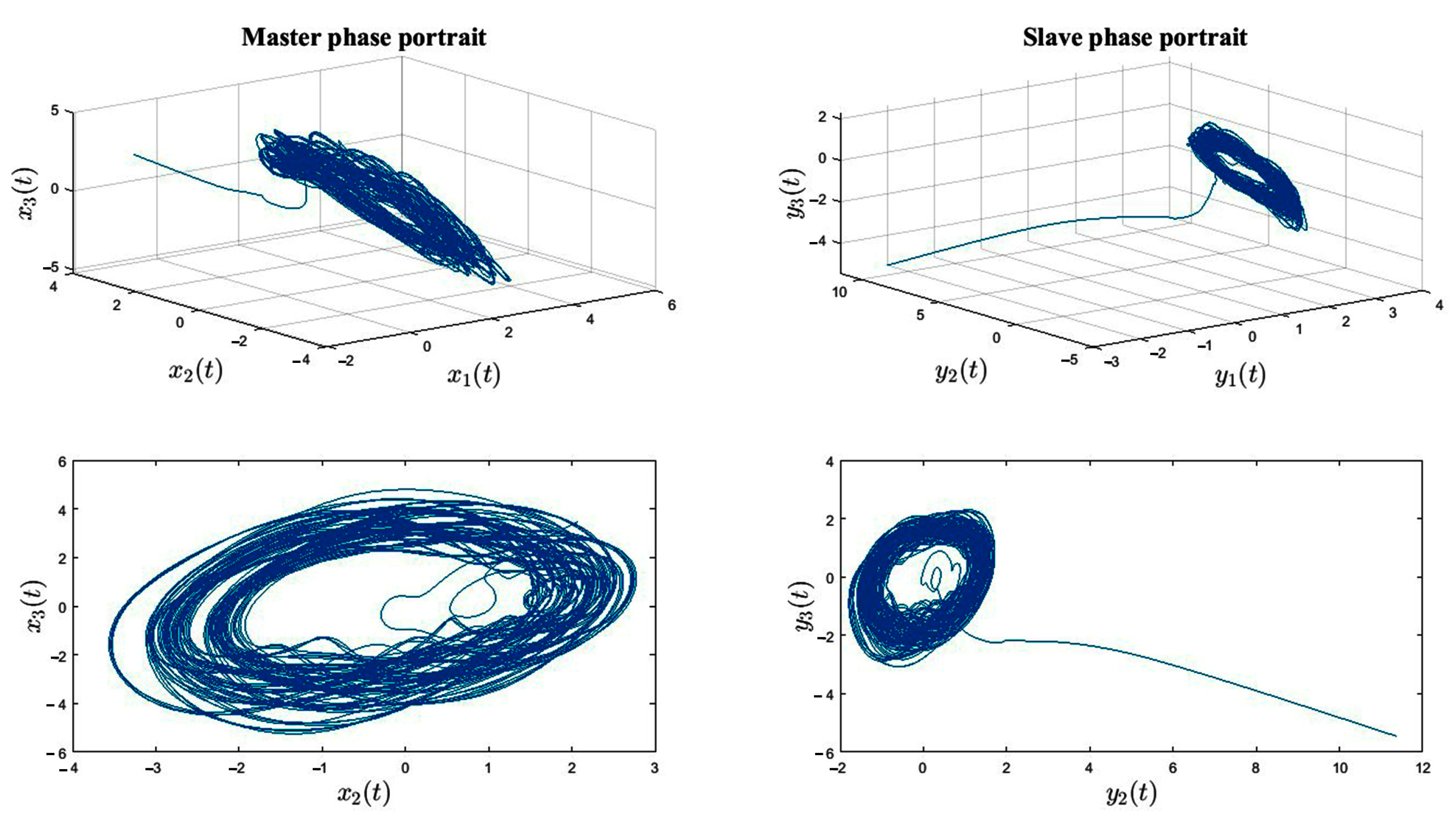
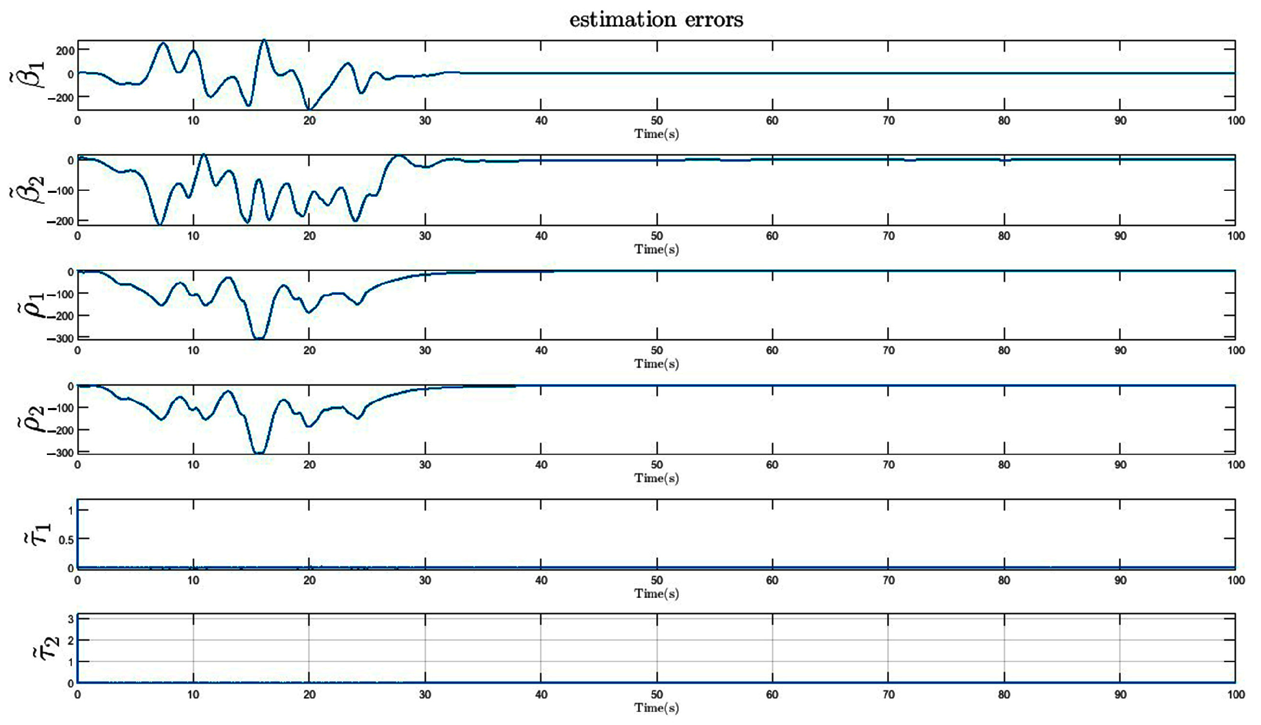
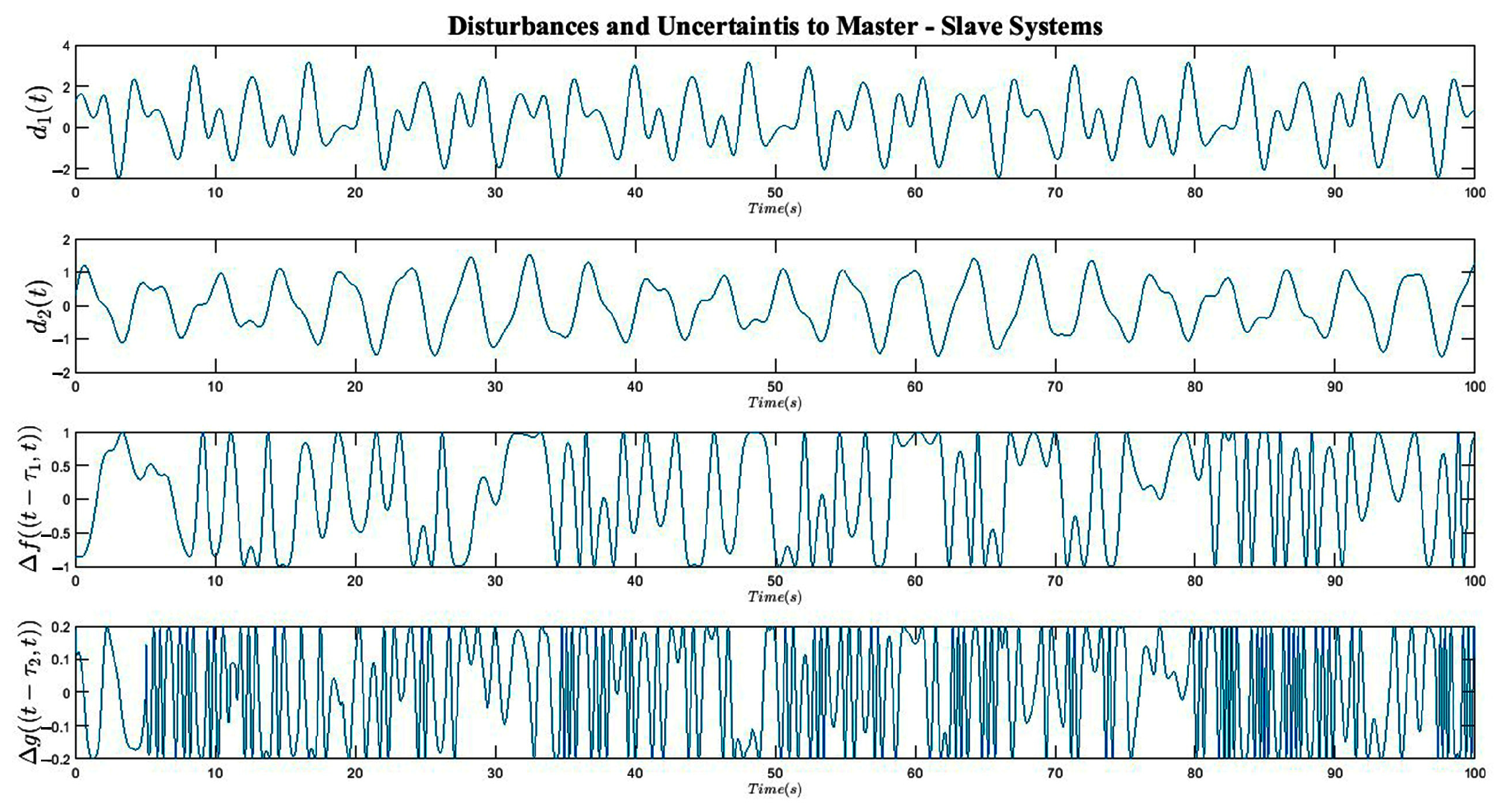
6. Simulation Results

In this section, the process of synchronizing time-varying chaotic systems with unknown uncertainty and time delay of the fractional order using the proposed control mechanism based on the nonlinear fractional order PID and with the advantage of the adaptive controller and update laws that estimate system parameters is verified, and its accuracy is evaluated. Two modified Jerk chaotic systems with the aforementioned characteristics were utilized for this purpose. The canonical form of the master system’s governing equations are as follows [15]:

$$\left\{\begin{array}{c}{D}^q{x}_1=x_2 \\ D^q{x}_2=x_3 \\ D^q{x}_3=-{\epsilon }_1{x}_1\left(t\right)-x_2\left(t\right)-{\epsilon }_2{x}_3\left(t\right)+f_3\left(x_1\left(t-{\tau }_1\right),t\right) \end{array}\right.$$

(51)

In this system, $f_3\left(x_1\left(t-{\tau }_1\right),t\right)$ is a piecewise linear function, as follows:

$$f_3\left(x_1\left(t-{\tau }_1\right),t\right)=\frac{1}{2}\left(v_0-v_1\right)\left[\left|x_1\left(t-{\tau }_1\right)+1\right|-\left|x_1\left(t-{\tau }_1\right)-1\right|\right]+v_1{x}_1\left(t-{\tau }_1\right)$$

(52)

Such that $v_0<-1<v_1<0$, $v_0=-2.5$, and $v_1=-0.5$.

Also, ${\epsilon }_i$ is a time-varying function, defined as follows.

$$\begin{array}{l}{\epsilon }_1\left(t\right)=0.5+0.3\sin \left(t\right)\cos \left(5\pi t\right)\\ {\epsilon }_2\left(t\right)=0.2+0.15\sin \left(0.5t\right)\cos \left(3\pi t\right)\end{array}$$

(53)

If ${\epsilon }_i\left(t\right)={\epsilon }_{0i}+∆{\epsilon }_i\left(t\right)$, $∆{\epsilon }_i\left(t\right)$ can be considered a part of the uncertainty and summed with the general uncertainty.

Thus, Equation (49) can be rewritten as follows:

$$\left\{\begin{array}{c}{D}^q{x}_1=x_2 \\ D^q{x}_2=x_3 \\ D^q{x}_3=-{ϵ}_{10}{x}_1\left(t\right)-x_2\left(t\right)-{ϵ}_{20}{x}_3\left(t\right)+f_3\left(x_1\left(t-{\tau }_1\right),t\right)\\ +{∆f}^{new}\left(x\left(t\right),t\right)+d_1\left(t\right).\end{array}\right.$$

(54)

in which ${∆f}^{new}(x\left(t\right),t))=∆f(x\left(t\right),t)-∆{\epsilon }_1\left(t\right)x_1\left(t\right)-∆{\epsilon }_2\left(t\right)x_3\left(t\right)$ with the previous structure. The same is carried out for the slave system.

When the initial conditions are chosen as ${\left(x_1\left(0\right);x_2\left(0\right);x_3\left(0\right)\right)}^T={\left(-0.5032;2.8545;-1.37\right)}^T$, the chaotic behavior of the system is as shown in Figure 2.

If the bounded uncertainty functions of the master and slave systems are as follows:

$$\begin{array}{l}∆f(x\left(t\right),t))=0.3sin\left(4x_1\left(t\right)+x_2\left(t\right)-x_3\left(t\right)\right)\\ ∆g(x\left(t\right),t))=0.2sin\left(y_1\left(t\right)+2y_2\left(t\right)-y_3\left(t\right)\right)\end{array}$$

(55)

The dynamic equations of the master and slave system are as follows:

$$\left\{\begin{array}{c}{D}^q{x}_1=x_2 \\ D^q{x}_2=x_3 \\ D^q{x}_3=-{\epsilon }_1{x}_1\left(t\right)-x_2\left(t\right)-{\epsilon }_2{x}_3\left(t\right)+f_3\left(x_1\left(t-{\tau }_1\right),t\right)\\ +{∆f}^{new}(x\left(t\right),t))+d_1\left(t\right) \end{array}\right.$$

(56)

The dynamic of the master system follows the following equations:

$$\left\{\begin{array}{c}{D}^q{y}_1=y_2 \\ D^q{y}_2=y_3 \\ D^q{y}_3=-{\epsilon }_1{y}_1\left(t\right)-y_2\left(t\right)-{\epsilon }_2{y}_3\left(t\right)+g_3\left(y_1\left(t-{\tau }_2\right),t\right)\\ +{∆g}^{new}(x\left(t\right),t))+d_2\left(t\right)+u\left(t\right) \end{array}\right.$$

(57)

Such that the nonlinear terms of the slave system are as follows:

$$g_3\left(y_1\left(t-{\tau }_2\right),t\right)=\frac{1}{2}\left(v_0-v_1\right)\left[\left|y_1\left(t-{\tau }_2\right)+1\right|-\left|y_1\left(t-{\tau }_2\right)-1\right|\right]+v_1{y}_1\left(t-{\tau }_2\right)$$

(58)

According to the dynamic of the master and slave systems described in Equations (51) and (52), the synchronization error is given as follows:

$$\left\{\begin{array}{c}{D}^q{e}_i=e_{i+1} 1\le i\le n-1\\ D^q{e}_n={\sigma }_0^T·e\left(t\right)+g\left(y\left(t-{\tau }_2\right),t\right)+∆g\left(y\left(t\right),t\right)+d_2\left(t\right)\\ -f\left(x_1\left(t-{\tau }_1\right)\right)-{∆f}^{new}(x\left(t\right),t))-d_1\left(t\right)+u\left(t\right) \end{array}\right.$$

(59)

Accordingly, the error dynamics for the chaotic Jerk system are as follows:

$$\left\{\begin{array}{c}{D}^q{e}_1=e_2 \\ D^q{e}_2=e_3 \\ D^q{e}_3=-{\epsilon }_1{e}_1\left(t\right)-e_2\left(t\right)-{\epsilon }_2{e}_3\left(t\right)-g\left(y_1\left(t-{\tau }_2\right)\right)+f\left(x_1\left(t-{\tau }_1\right)\right) \\ +{∆g}^{new}(x\left(t\right),t))-{∆f}^{new}(x\left(t\right),t\left)\right)\\ d_2\left(t\right)-d_1\left(t\right)+u\left(t\right) \end{array}\right.$$

(60)

At this stage, we applied the robust adaptive control signal, which is devised by combining the sliding surface based on the structure of the fractional order nonlinear PID controllers and described in Equation (26), to the slave system.

In this article, simulations were run for 100 s. Figure 2 depicts the master and slave systems in three-dimensional space. Figure 3 illustrates the behavior of the master and slave system states in the absence of any controller actions. Figure 4 shows the synchronization of the master and slave system. It is clear that after applying the control signal based on the proposed mechanism, the slave system follows the master system well. Figure 5 depicts the synchronization error of the master and slave system utilizing the proposed mechanism. Figure 6 depicts the control signal based on the proposed method. According to the range of the image’s control signal (6), it is unquestionable that the proposed controller can be implemented. As this figure demonstrates, the controller signal exhibited no chattering, and a saturation limit of 24 volts was used, which is simple to implement. In this design, the controller coefficients $k_{11}=k_{22}=9$ and $k_{12}=k_{21}=18$ were selected. Also, the gain and time constants of the PID sliding surface are nonlinear fractional orders, as $k_p=3$, $T_i=0.8$, and $T_d=0.65$. The fractional order of the integral part and the derivative of the sliding surface are defined as $\delta =0.15$ and $\lambda =0.75$. The parameters of the proposed robust controller are $\overline{ϵ}=0.01$ and $b=2$. The unknown time delays of the system are ${\tau }_1=0.3$ and ${\tau }_2=0.5$. The time delay of the master system changes to the value of ${\tau }_1=0.45$ at the moment $t=40$ s, and the time delay of the follower system changes to the value of ${\tau }_2=0.58$ at the moment $t=50$ s. The error in estimating the uncertainty, disturbance, and delay bounds is shown in Figure 7. Figure 8 shows the uncertainties and disturbances applied to the master and slave systems. The unknown disturbances are applied to both systems as follows:

$$\begin{array}{l}{d}_1\left(t\right)=0.8{sin}^{2}2t+1.2cos3t+1.6sin1.3t\\ d_2\left(t\right)=sin1.4t+0.3sin\pi t+0.3cos\frac{\pi t}{2} \end{array}$$

(61)

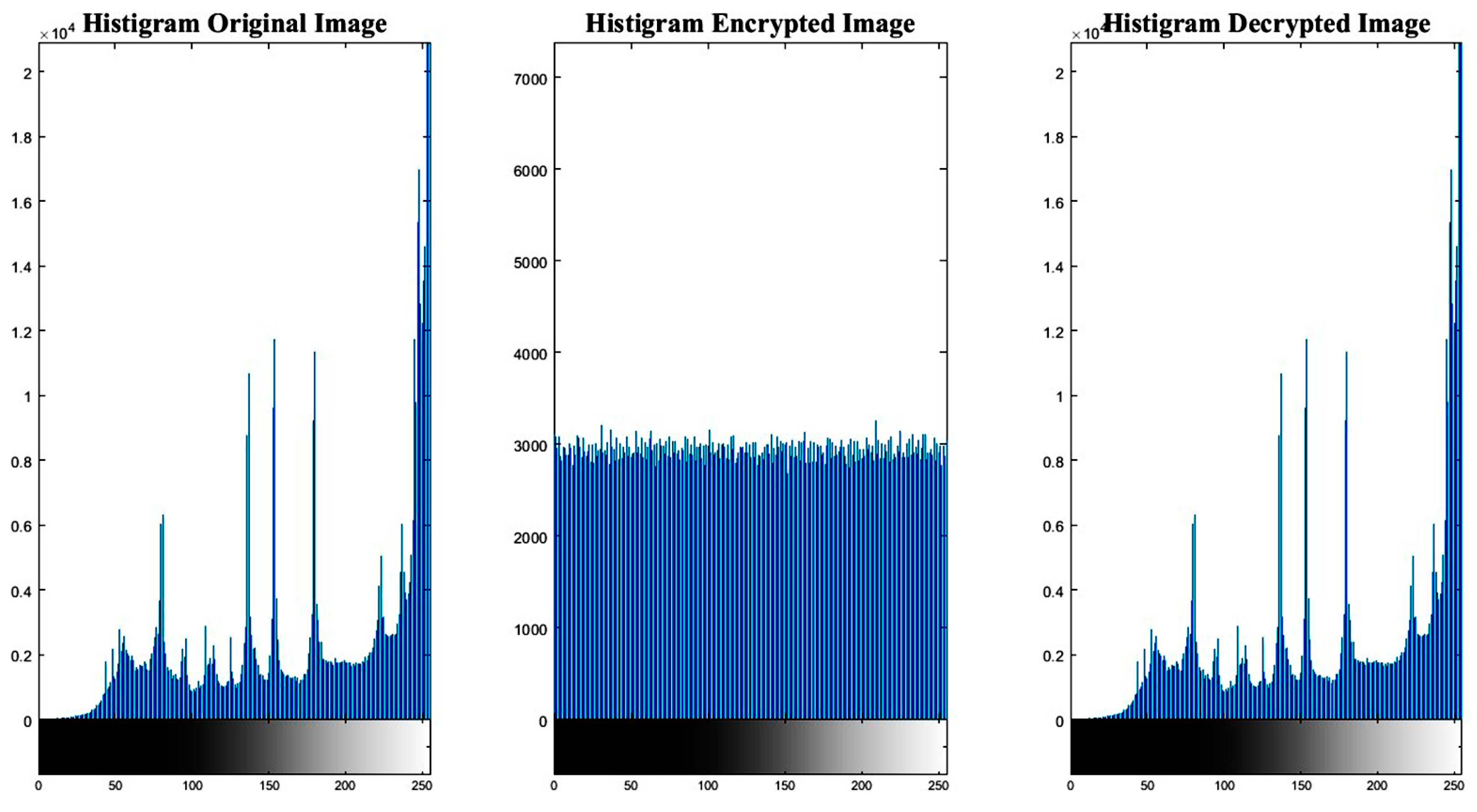
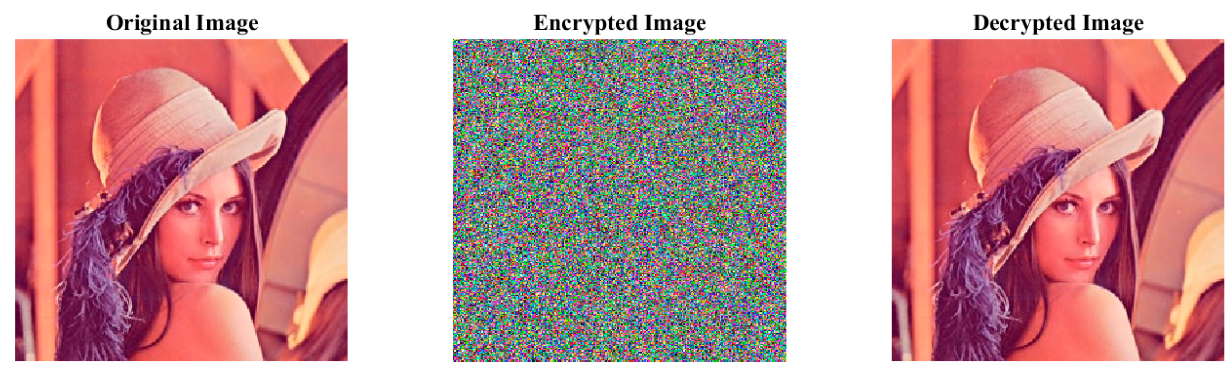
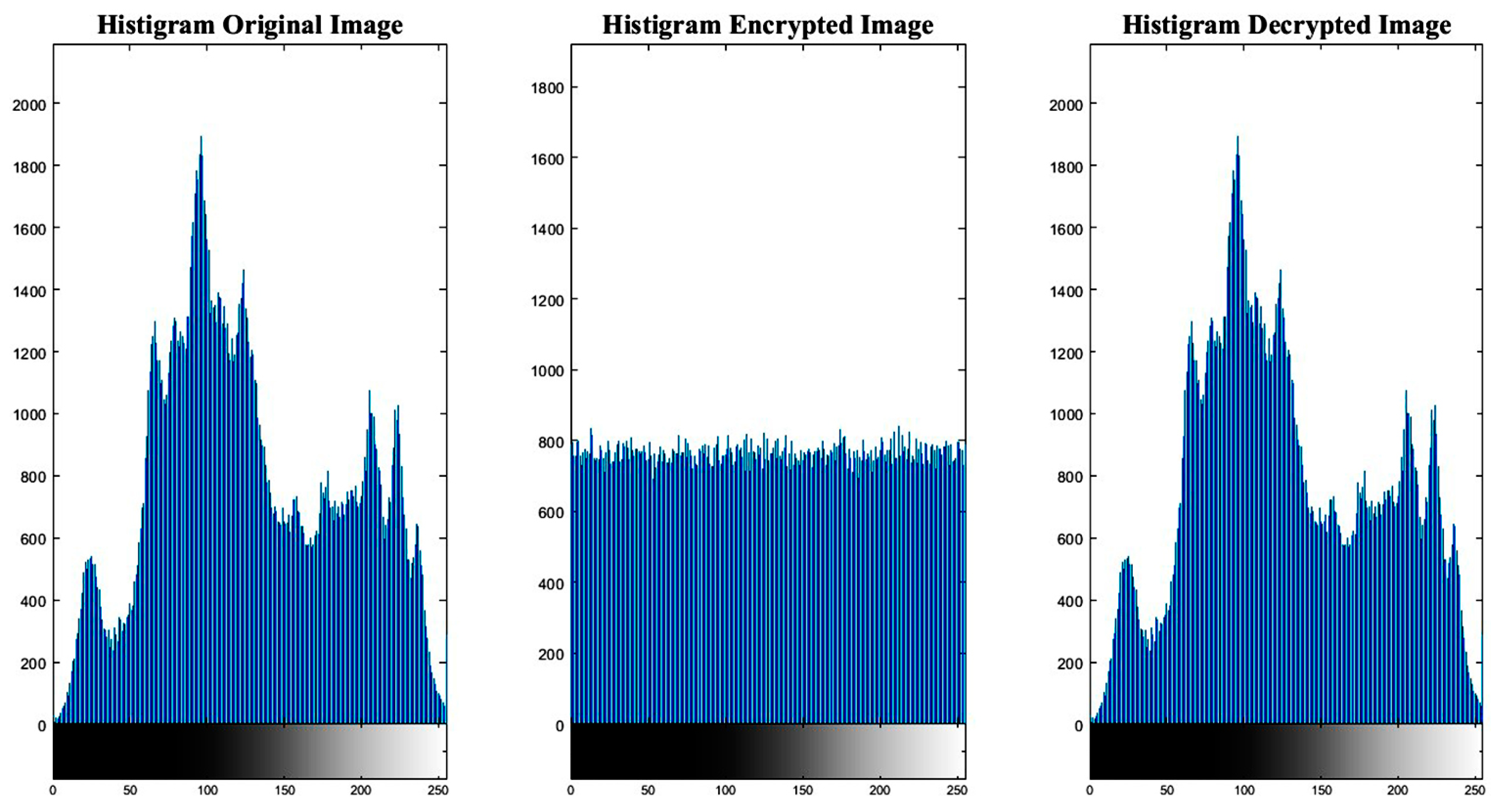
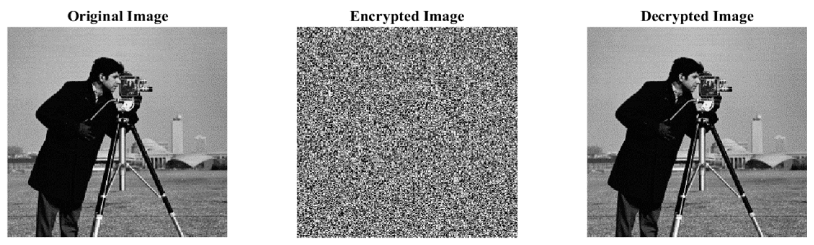
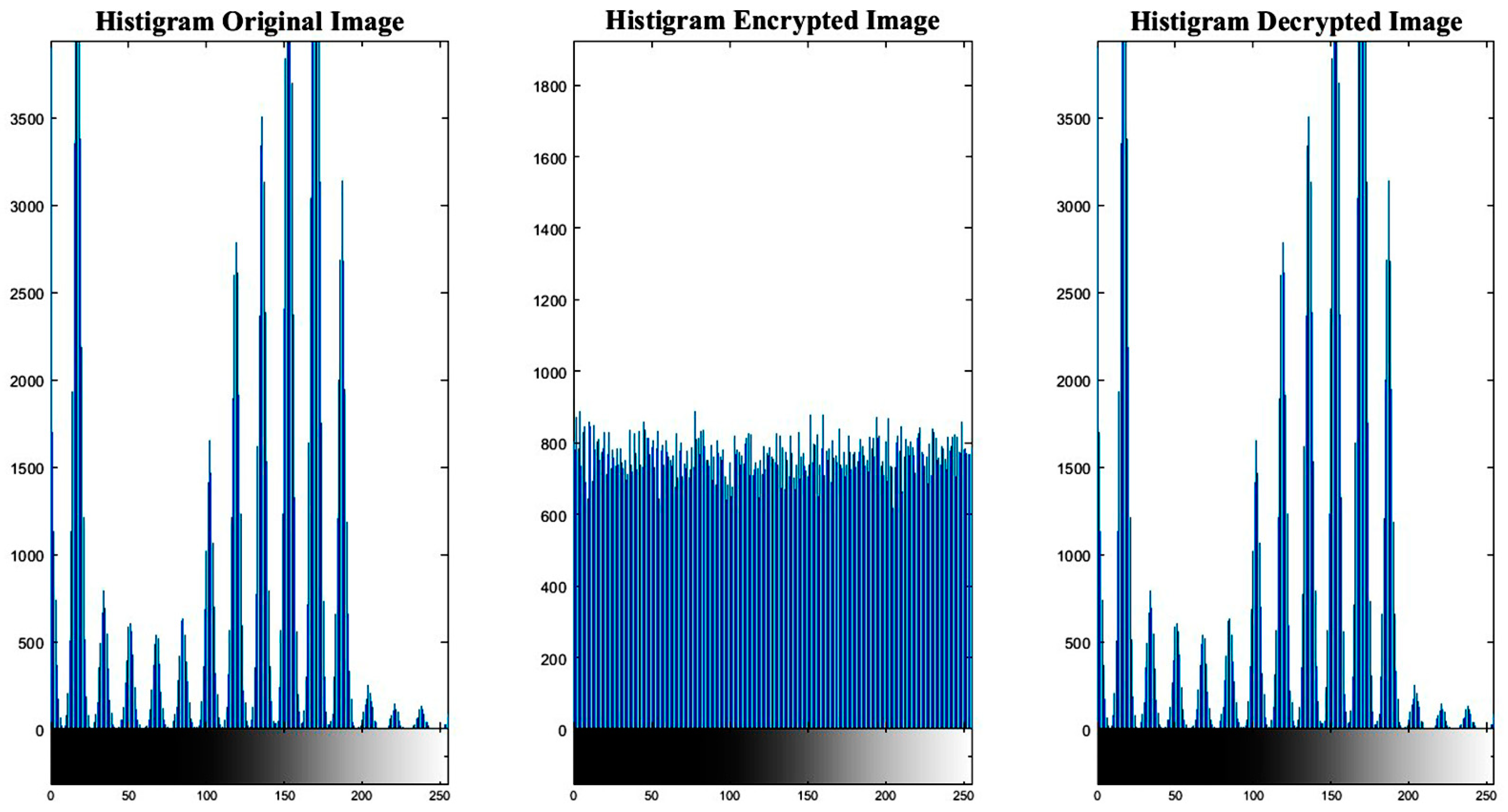
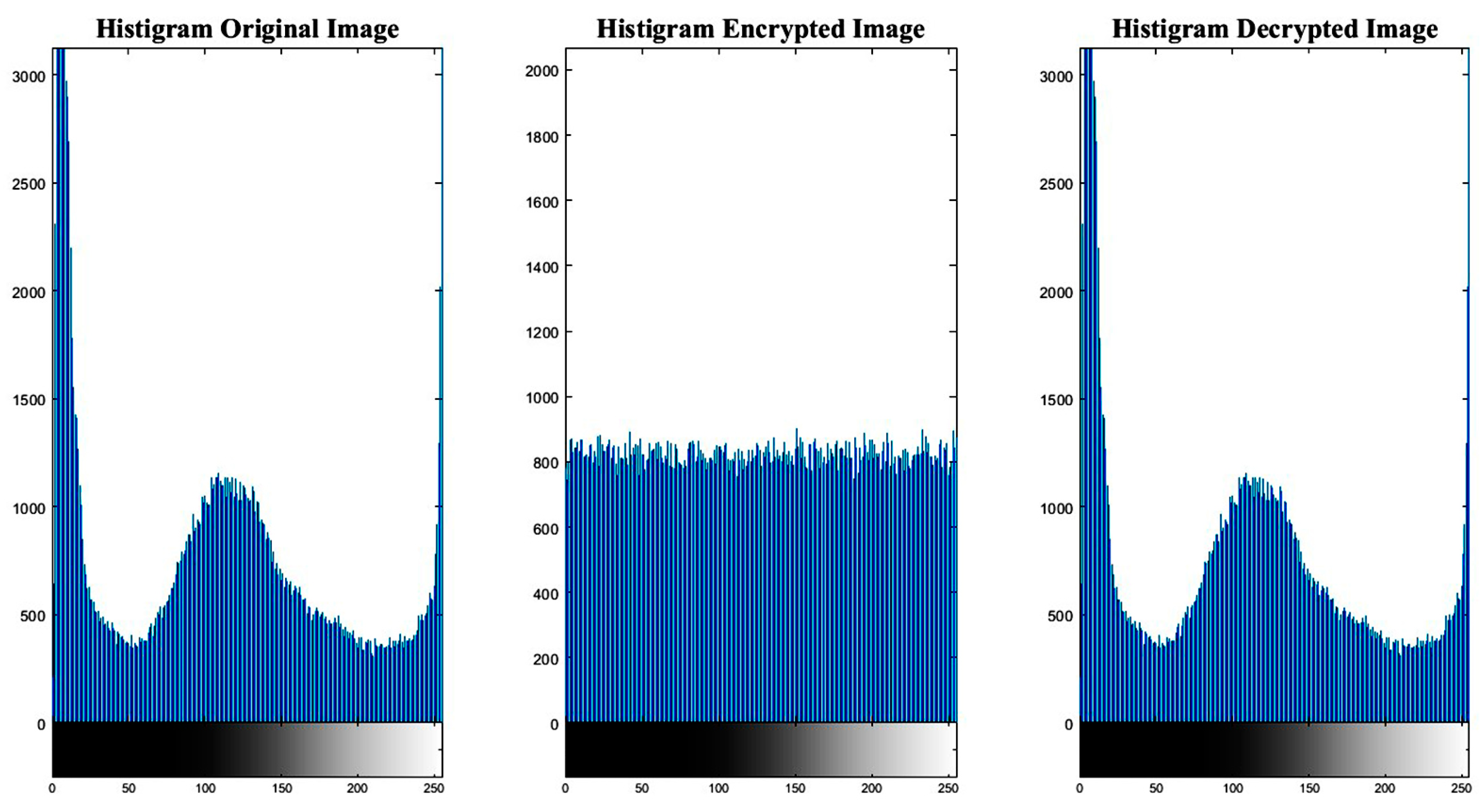
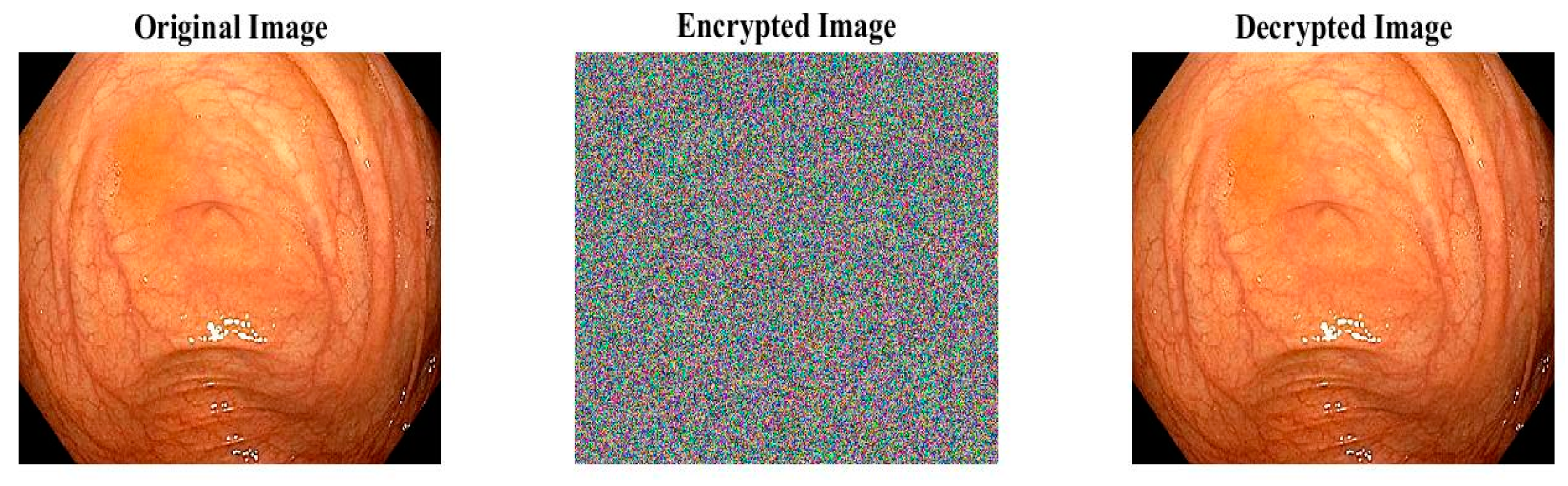
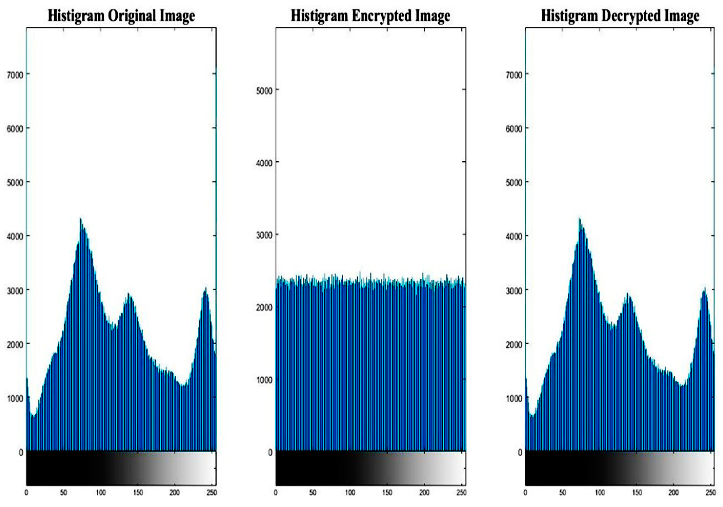
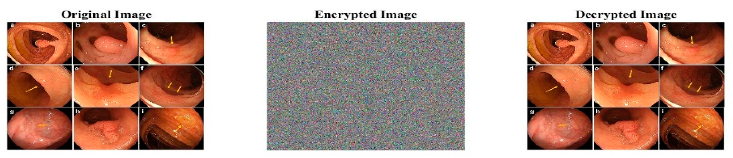
7. Application of Secure Communication in Encryption and Image Retrieval

Despite the uncertainties and time delays in the system, the fractional order chaotic master and slave systems were entirely synchronized according to the proposed mechanism, the details of which were described in the previous section. Images were encrypted using the [27] algorithm in this section. The encrypted image was then transmitted using fractional order chaotic masking and received with high precision before being decoded.

Figure 9 is a block diagram detailing the encryption technique applied to the images. In this block diagram, information is exchanged via a wireless communication channel.

Various statistical parameters, including the histogram difference between the original image and the restored image, correlation, NPCR, PSNR, and information entropy, were calculated for standard color benchmark images and medical color images to demonstrate the efficacy of the proposed method. These parameters are standard criteria that have been used in numerous articles [27].

This section encrypts images for secure communication utilizing the mechanism whose efficacy was evaluated in Section 6. Figure 10 shows the result of image encryption and recovery using secure communication for the original image, and Figure 11 shows their histogram for Aletta (Isekai.Shokudou) color image.

Figure 12 shows the encryption on the lena color image and Figure 13 shows its histogram.

It can be seen that the decoded images were well restored using the proposed synchronization scheme.

Table 2. Results of statistical criteria of color images.

Images	Histogram		Correlation	Differential Attack		PSNR	Information Entropy
	Standard	Encrypted		NPCR (%)	UACI (%)
Images 10	21,153.1171	21,148.239	0.0068	99.68	33.23	8.10	7.9690
Images 12	18,144.3510	18,143.750	0.0043	99.40	33.46	8.27	7.9700

shows the results of the statistical criteria of Figure 10 and Figure 12.

Image encryption using the above mechanism along with histogram for cameraman’s black and white image is shown in Figure 14 and Figure 15, respectively, and for panda is presented in Figure 16 and Figure 17.

Table 3. Results of statistical measures of black and white images.

Images	Histogram		Correlation	Differential Attack		PSNR	Information Entropy
	Main	Decoded		NPCR (%)	UACI (%)
Images 14	398,232.09375	398,201.1053	0.9923	99.21	33.55	8.9671	7.9783
Images 16	24,466.718750	24,421.32934	0.9953	99.48	33.21	8.0221	7.9458

shows the results of the statistical criteria of the black and white images in Figure 14 and Figure 16.

The encryption of the medical color image along with its histogram for the single image mode is shown in Figure 18 and Figure 19 and for the multiple image in Figure 20 and Figure 21, respectively.

Table 4. Results of statistical measures of medical images.

Images	Histogram		Correlation	Differential Attack		PSNR	Information Entropy
	Standard	Decrypted		NPCR (%)	UACI (%)
Images 18	65,536	65,535	0.9986	99.96	33.46	9.23	7.9627
Images 20	65,536	65,534	0.9987	99.97	33.47	9.24	7.9842

shows the results of the statistical criteria of the color medical images in Figure 18 and Figure 20. The results of encryption entropy indicate excellent quality of image retrieval.

8. Conclusions

This study examined a novel adaptive sliding mode control approach for robust synchronization of a class of fractional order chaotic systems with uncertainty, external disturbance, and unknown parameters, such as unknown time delay. In the proposed robust control mechanism, a nonlinear fractional order sliding surface was first proposed based on the structure of nonlinear proportional, integral, and fractional derivative controllers. Using the Lyapunov theory and Lipschitz conditions in chaotic systems, matching criteria were established in order to estimate the unknown parameters of the system. In order to facilitate the implementation process, the control signal’s saturation limit was defined, and the robust control system’s stability was demonstrated. The synchronization of two fractional order Jerk chaotic systems with the stated characteristics, including uncertainties and unknown time delays, based on the proposed control mechanism was simulated using MATLAB, and the results express the capability and optimal performance of the proposed approach in the robust synchronization of the mentioned systems. In closing, the proposed adaptive sliding mode control approach was implemented in the structure of a chaotic secure communication mechanism, and the simulation results indicate a high level of quality in the secure encryption and decryption of digital images despite the presence of uncertain parameters in the master and slave systems of the communication mechanism.

References

1. Lorenz, E.N. Deterministic Non-Periodic Flow. J. Atmos. Sci. 1963, 20, 130–141. [Google Scholar] [CrossRef]
2. Chen, G.R.; Ueta, T. Yet Another Chaotic Attractor. Int. J. Bifurc. Chaos Appl. Sci. Eng. 1999, 9, 1465–1466. [Google Scholar] [CrossRef]
3. Lü, J.H.; Chen, G.R. A New Chaotic Attractor Coined. Int. J. Bifurc. Chaos Appl. Sci. Eng. 2002, 12, 659–661. [Google Scholar] [CrossRef]
4. Liu, C.X.; Liu, T.; Liu, L.; Liu, K. A New Chaotic Attractor. Chaos Solitons Fractals 2004, 22, 1031–1038. [Google Scholar] [CrossRef]
5. Fernandez, A.; Baleanu, D.; Srivastava, H. Series representations for fractionalcalculus operators involving generalised Mittag-Leffler functions. Commun. Nonlinear Sci. Numer. Simul. 2019, 67, 517–527. [Google Scholar] [CrossRef]
6. Zhang, J.; Gao, F.; Chen, Y.; Zou, Y. Parameter identification of fractional-order chaotic system based on chemical reaction optimization. In Proceedings of the 2018 2nd International Conference on Management Engineering, Software Engineering and Service Sciences, New York, NY, USA, 13–15 January 2018; pp. 217–222. [Google Scholar]
7. Ionescu, C.; Lopes, A.; Copot, D.; Machado, J.T.; Bates, J. The role of fractionalcalculus in modeling biological phenomena: A review. Commun. Nonlinear Sci. Numer. Simul. 2017, 51, 141–159. [Google Scholar] [CrossRef]
8. Smida, M.B.; Sakly, A.; Vaidyanathan, S.; Azar, A.T. Control-based maximum power point tracking for a grid-connected hybrid renewable energy system optimized by particle swarm optimization. In Advances in System Dynamics and Control; Tomorrow’s Research Today: Rochester, NY, USA, 2018; pp. 58–89. [Google Scholar]
9. Vinagre, B.; Feliu, V. Modeling and control of dynamic system using fractional calculus: Application to lectrochemical processes and flexible structures. In Proceedings of the 41st IEEE Conference on Decision and Control, Las Vegas, NV, USA, 10–13 December 2002; Volume 1, pp. 214–239. [Google Scholar]
10. Li, R.-G.; Wu, H.-N. Secure communication on fractionalorder chaotic systems via adaptive sliding mode control with teaching–learning–feedback-based optimization. Nonlinear Dyn. 2018, 92, 1221–1243. [Google Scholar]
11. Mandelbrot, B.B.; Van Ness, J.W. Fractional Brownian motions, fractional noises and applications. SIAM Rev. 1968, 10, 422–437. [Google Scholar] [CrossRef]
12. Duarte, F.B.; Machado, J.T. Chaotic phenomena and fractional-order dynamics in the trajectory control of redundant manipulators. Nonlinear Dyn. 2002, 29, 315–342. [Google Scholar] [CrossRef]
13. Petráš, I. Fractional-order nonlinear controllers: Design and implementation notes. In Proceedings of the 2016 17th International Carpathian Control Conference (ICCC), High Tatras, Slovakia, 29 May–1 June 2016; IEEE: Piscataway, NJ, USA, 2016; pp. 579–583. [Google Scholar]
14. Mirrezapour, S.Z.; Zare, A. A new fractional sliding mode controller based on nonlinear fractional-order proportional integral derivative controller structure to synchronize fractional-order chaotic systems with uncertainty and disturbances. J. Vib. Control. 2021, 28, 1–13. [Google Scholar] [CrossRef]
15. Zare, A.; Mirrezapour, S.Z.; Hallaji, M.; Shoeibi, A.; Jafari, M.; Ghassemi, N.; Alizadehsani, R.; Mosavi, A. Robust Adaptive Synchronization of a Class of Uncertain Chaotic Systems with Unknown Time-Delay. Appl. Sci. 2020, 10, 8875. [Google Scholar] [CrossRef]
16. Mohammadpour, S.; Binazadeh, T. Robust Observer-Based Synchronization of Unified Chaotic Systems in the Presence of Dead-Zone Nonlinearity Input. J. Control Iran. Soc. Instrum. Control Eng. (ISICE) 2018, 11, 25–36. [Google Scholar]
17. Modiri, A.; Mobayen, S. Adaptive terminal sliding mode control scheme for synchronization of fractional-order uncertain chaotic systems. ISA Trans. 2020, 105, 33–50. [Google Scholar] [CrossRef]
18. Mostafaee, J.; Mobayen, S.; Vaseghi, B.; Vahedi, M. Dynamical Analysis and Finite-Time Fast Synchronization of a Novel Autonomous Hyper-Chaotic System. J. Intell. Proced. Electr. Technol. 2021, 12, 47. [Google Scholar]
19. Rasouli, M.; Zare, A.; Hallaji, M.; Alizadehsani, R. The Synchronization of a Class of Time-Delayed Chaotic Systems Using Sliding Mode Control Based on a Fractional-Order Nonlinear PID Sliding Surface and Its Application in Secure Communication. Axioms 2022, 11, 738. [Google Scholar] [CrossRef]
20. Aghababa, M.P. Finite-time chaos control and synchronization of fractional order nonautonomous chaotic (hyperchaotic) systems using fractional nonsingular terminal sliding mode technique. Nonlinear Dynam. 2012, 69, 247–261. [Google Scholar] [CrossRef]
21. Balochian, S.; Sedigh, A.K.; Zare, A. Variable structure control of linear time invariant fractional order systems using a finite number of state feedback law. Commun. Nonlinear Sci. Numer. Simul. 2011, 16, 1433–1442. [Google Scholar] [CrossRef]
22. Chen, W.; Dai, H.; Song, Y.; Zhang, Z. Convex Lyapunov functions for stability analysis of fractional order systems. IET Control Theory Appl. 2017, 11, 1070–1074. [Google Scholar] [CrossRef]
23. Aguila-Camacho, N.; Duarte-Mermoud, M.A.; Gallegos, J.A. Lyapunov functions for fractional order systems. Commun. Nonlinear Sci. Numer. Simul. 2014, 19, 2951–2957. [Google Scholar] [CrossRef]
24. Chen, X.; Park, J.H.; Cao, J.; Qiu, J. Sliding mode synchronization of multiple chaotic systems with uncertainties and disturbances. Appl. Math. Comput. 2017, 308, 161–173. [Google Scholar] [CrossRef]
25. Draa, K.C.; Zemouche, A.; Alma, M.; Voos, H.; Darouach, M. New Trends in Observer-Based Control a Practical Guide to Process and Engineering Applications; Elsevier: Amsterdam, The Netherlands, 2019; pp. 99–135. [Google Scholar]
26. Petras, I. Fractional-Order Nonlinear Systems: Modeling, Analysis and Simulation; Springer Science & Business Media: Berlin/Heidelberg, Germany, 2011. [Google Scholar]
27. Kekha Javan, A.A.; Zare, A.; Alizadehsani, R. Multi-State Synchronization of Chaotic Systems with Distributed Fractional Order Derivatives and Its Application in Secure Communications. Big Data Cogn. Comput. 2022, 6, 82. [Google Scholar] [CrossRef]
Figure 1. Sigma function behavior diagram.
Axioms 12 00828 g001
Figure 2. Chaotic behavior of the fractional order Jerk master and slave systems without applying the controller.
Axioms 12 00828 g002
Figure 3. The behavior of the master and slave system states without applying the control signal.
Axioms 12 00828 g003
Figure 4. Synchronization of chaotic jerk systems with the help of the proposed control mechanism and application of the control signal at t = 5 s.
Axioms 12 00828 g004
Figure 5. Synchronization error of the master and slave systems using the proposed adaptive sliding mode control mechanism.
Axioms 12 00828 g005
Figure 6. Control signal based on the proposed adaptive sliding mode control mechanism.
Axioms 12 00828 g006
Figure 7. System parameter estimation error including time delay, disturbance bound, and uncertainty bound.
Axioms 12 00828 g007
Figure 8. Uncertainties and disturbances in the master and slave systems.
Axioms 12 00828 g008
Figure 9. Block diagram of chaotic masking for image encryption.
Axioms 12 00828 g009
Figure 10. The original, encrypted, and decrypted color image.
Axioms 12 00828 g010
Figure 11. Histogram of the original, encrypted, and decrypted color image.
Axioms 12 00828 g011
Figure 12. Original, encrypted, and decrypted color image.
Axioms 12 00828 g012
Figure 13. Histogram of the original, encrypted, and decrypted color image.
Axioms 12 00828 g013
Figure 14. The original, encrypted, and decrypted black and white image.
Axioms 12 00828 g014
Figure 15. Histogram of the original, encrypted, and decrypted black and white image.
Axioms 12 00828 g015
Figure 16. The original, encrypted, and decrypted black and white image.
Axioms 12 00828 g016
Figure 17. Histogram of the original, encrypted, and decrypted black and white image.
Axioms 12 00828 g017
Figure 18. Original, encrypted, and decrypted medical image.
Axioms 12 00828 g018
Figure 19. Histogram of the original, encrypted, and decrypted medical image.
Axioms 12 00828 g019
Figure 20. The original, encrypted, and decrypted medical image.
Axioms 12 00828 g020
Figure 21. Histogram of the original, encrypted, and decrypted medical image.
Axioms 12 00828 g021