1. Introduction
In this article, we study Neural Networks, called also Artificial Neural Networks (ANN), and their mathematical models, using ordinary differential equations. The motivation for the study of ANNs came from attempts to understand the principles and organization of the human brain. Understanding came that human brains work differently from digital computers. Their effectiveness comes from high complexity, nonlinear modes of regulation, and parallelism of actions. The elements of the human brain were called neurons.
These elements still perform calculations faster than the fastest digital computers. The human brain is able to perceive information about the environment in the form of images and, moreover, it can process the received information needed for interaction with the environment.
At birth, the human brain has a ready structure for learning which, in familiar terms, is understood as experience. So, the neural network is designed to model the way in which the human brain solves usual problems and performs a particular task. A particular interest in ANN stems from the fact that an important group of neural networks is needed to solve a problem computations through the process of learning. So, following [
1], an ANN can generally be imagined as a parallel distributed processor, consisting of separate units, which is able to analyze experimental data and prepare them for use.
Many natural processes involve networks of elements that affect each other following a general pattern of conditions and the updating rules for any elements. Both genomic networks and neuronal networks are of this kind. In mathematical models of networks of both types, the regulatory effect of one element to the outputs of other elements is defined by a weight matrix. Therefore, the models describing the evolution of these networks have a lot in common. But, there are also differences. This paper compares models using systems of ordinary differential equations. To distinguish between these systems, we use the designations GRN system and ANN system. At the same time, we realize that the term ANN system has too general a meaning. An ANN system in the established sense is understood as a network that operates according to certain rules and is focused on performing certain tasks. At the same time, the networks undergo training and thus improve their qualities. This article looks at neural networks from a different point of view. We are interested in the behavior of systems of both types for different forms of interaction of elements. The structure of both systems assumes the presence of attractors that determine future states. The description and comparison of possible attractors for the systems of both types is our result.
ANNs are made up of many interconnected elements. Weighted signals from different elements are received by a separate element and processed. A positive signal is understood as an excitatory connection, while negative one means an inhibitory connection. The received signals are linearly summed and modified by a nonlinear sigmoidal function which is called an activation one. The activation function controls the amplitude of an output. “Each neuron has a sigmoid transfer function, and a continuous positive and bounded output activity that evolves according to weighted sums of the activities in the networks. Neural networks with arbitrary connections are often called recurrent networks” [
2]. The dynamics of the continuous time recurrent neural network with
n units, can be described by the system of ordinary differential equations (ODE) ([
3])
where
is the internal state of the
i-th unit,
is the time constant for the
i-th unit,
are connection weights,
is the input to the
i-th unit, and
is the response function of the
i-th unit. Usually,
f is taken as a sigmoidal function. There are particular response functions that are non-negative. For instance, functions
were used in [
4]. More general cases can be modeled by the system using the function
which takes values in the open interval
If the recurrent neural networks without input are considered, the system
can be considered.
Applications of Artificial Neural Networks are multiple. They can be used in different fields. These fields can be categorized as function approximations, including time series prediction and modeling; pattern and sequence recognition, novelty detection and sequential decision making; and data processing, including filtering and clustering. For applications in Machine Learning (ML), Deep Learning and related problems, consult the review article [
5]. For neuroscience applications and their relation to ML, and machine learning using biologically realistic models of neurons to carry out the computation, consider the review [
6]. The problems of pattern recognition by ANNs, including applications in manufacturing industries, were studied and analyzed in the review paper [
7]. In the paper [
8], the ANN approach is applied for the study of a genetic system.
In this article, we mainly study properties of the mathematical model of a three-dimensional ANN, but part of our results will refer to two-dimensional or, more generally, to
n-dimensional networks. In particular, we provide information on the types of possible attractors, and their birth and evolution under changes in multiple parameters. The asymptotic properties of the system are important for prediction of future states. This, in turn, can provide instruments for control and management of the modeling network. We use analytical tools for the study of the phase space and its elements. A set of formulas is obtained for the local analysis near equilibria. The necessary data for the analysis were collected by conducting computational experiments and constructing several examples. A broader study involves examining the model and interpreting the findings for the actual process being modeled. Examples of this approach are the works [
9,
10].
Let us describe the structure of the paper. The Problem formulation section provides the necessary material for the study. The Preliminary results section describes some basic properties of the main systems of ordinary differential equations. It deals also with technical details concerning nullclines, critical points, local analysis by linearization, and some special cases. The next two sections concern some particular but important cases. The systems possessing critical points of the type focus, and systems exhibiting the inhibition-activation behavior, are treated. Both types of systems can have periodic solutions, and that means that cyclic processes can occur in the modeled network. The system of the special triangular structure is analyzed in
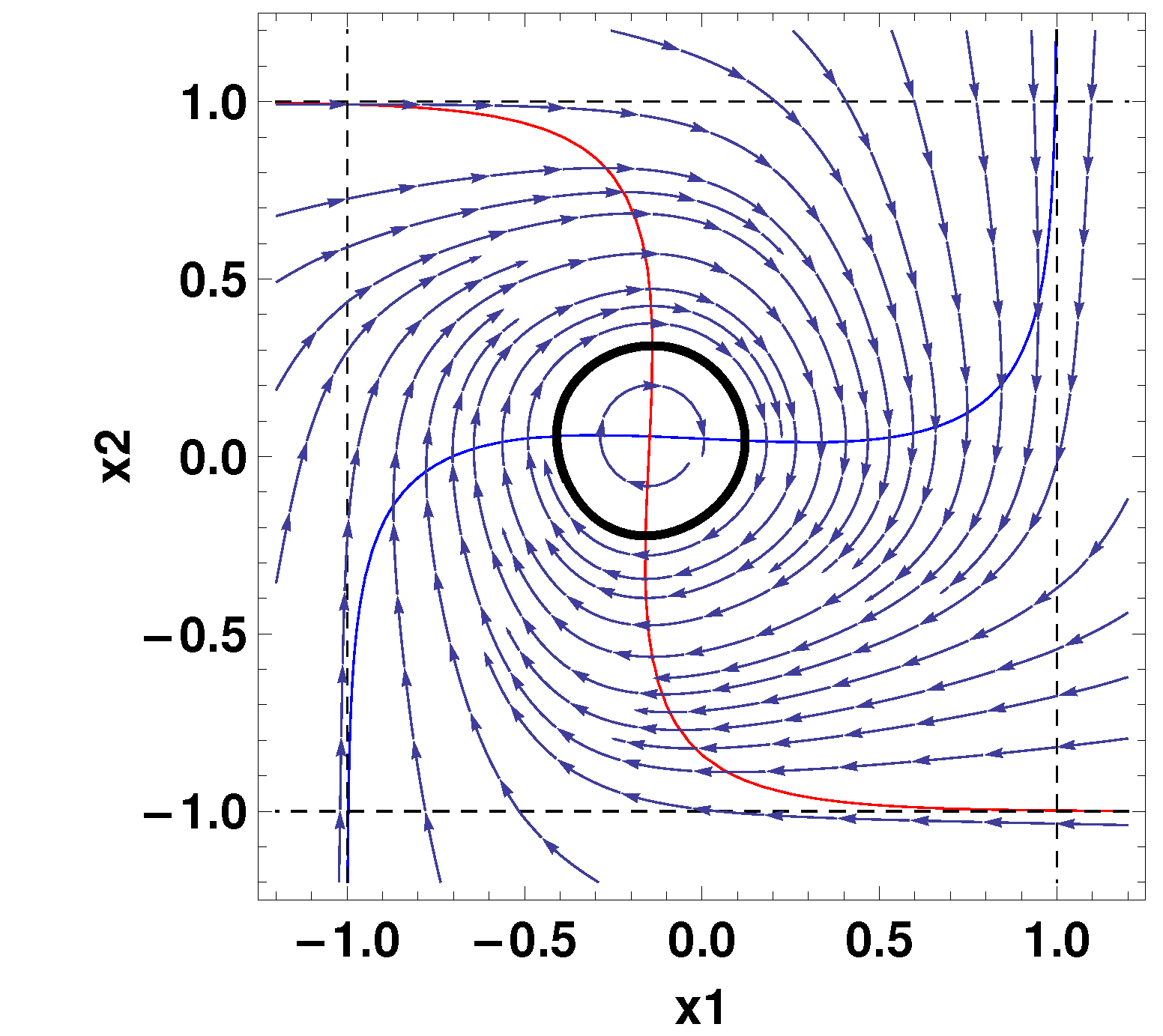
Section 6. It is convenient for analysis and the main conclusions can be transferred to systems of arbitrary dimensions. The process of birth of stable periodic trajectories from stable critical points of the type focus is considered in
Section 7. The mechanism of the Andronov–Hopf bifurcation is illustrated for two-dimensional and three-dimensional neuronal systems. As a by-product, an example of a 3D system that has three limit cycles is constructed. Some suggestions on the management of neuronal systems are provided in
Section 7. The possibility of effectively changing the properties of the system, and therefore to partially controlling the network in question, is emphasized. The last section summarizes the results obtained so far, and outlines further studies in this direction.
2. Problem Formulation
The mathematical model using ordinary differential equations, is
The same system can be written as ([
11])
since
The elements of this 3D network are called neurons. The connections between them are synapses (or nerves). There is an algorithm that describes how the impulses are propagated through the network. In the above model, this algorithm is encoded by the matrix
Each neuron accepts signals from others and produces a single output. The extent to which the input of neuron i is driven by the output of neuron j is characterized by its output and synaptic weight
The dynamic evolution leads to attractors of the system (
4), and it was experimentally observed in neural systems. In theoretical modeling, the emphasis is put on the attractors of a system. We wish to study them for System (
4).
Similar systems arise in the theory of genetic regulatory networks. The difference is that the nonlinearity is represented by a positive valued sigmoidal functions. One of such systems is
Notice that System (
3), and therefore also System (
4), can be obtained from System (
6), where
by two arithmetic operations, namely multiplication of the nonlinearity in (
6) by 2 and subtracting 1. This changes the range of values in (
3) to
Systems of the form (
6) were studied before by many authors. The interested reader may consult the works ([
12,
13,
14,
15,
16,
17,
18,
19,
20]). Similar systems appear in the theory of telecommunication networks ([
21]).
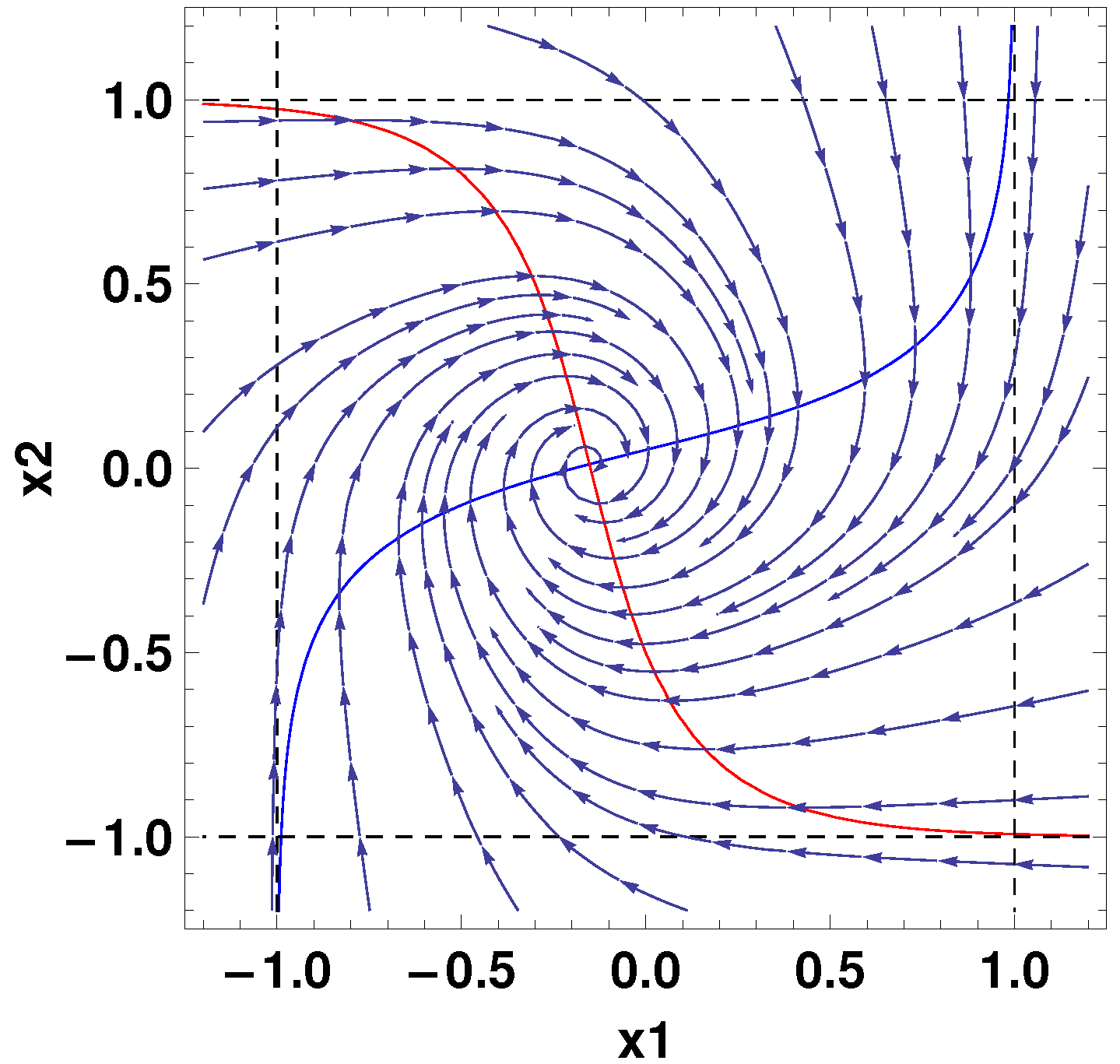
In this article, we study the different dynamic regimes for System (
4) which can be observed under various conditions. In particular, we first speak about critical points in System (
4) and evaluate the number of them. Then, we focus on periodic regimes, study their attractiveness for other trajectories. This can be performed, under some restrictions, for systems of relatively high dimensionality. Also, the evidences of chaotic behavior are presented.
8. Control and Management of ANN
First, a citation from [
22]: “Models of ANN are specified by three basic entities: models of the neurons themselves–that is, the node characteristics; models of synaptic interconnections and structures–that is, net topology and weights; and training or learning rules—that is, the method of adjusting the weights or the way the network interprets the information it receives”.
In this section, we discuss the problem of changing the behavior of the trajectories of System (
4). This may be interpreted as partial control over the system. The system has as parameters the coefficients
the values
and
in the linear part. Properties of the system may be changed by varying any of mentioned.
We would like demonstrate how a system of the form (
4) can be modified so that trajectories start to tend to some of indicated attractor. For this, consider the system (
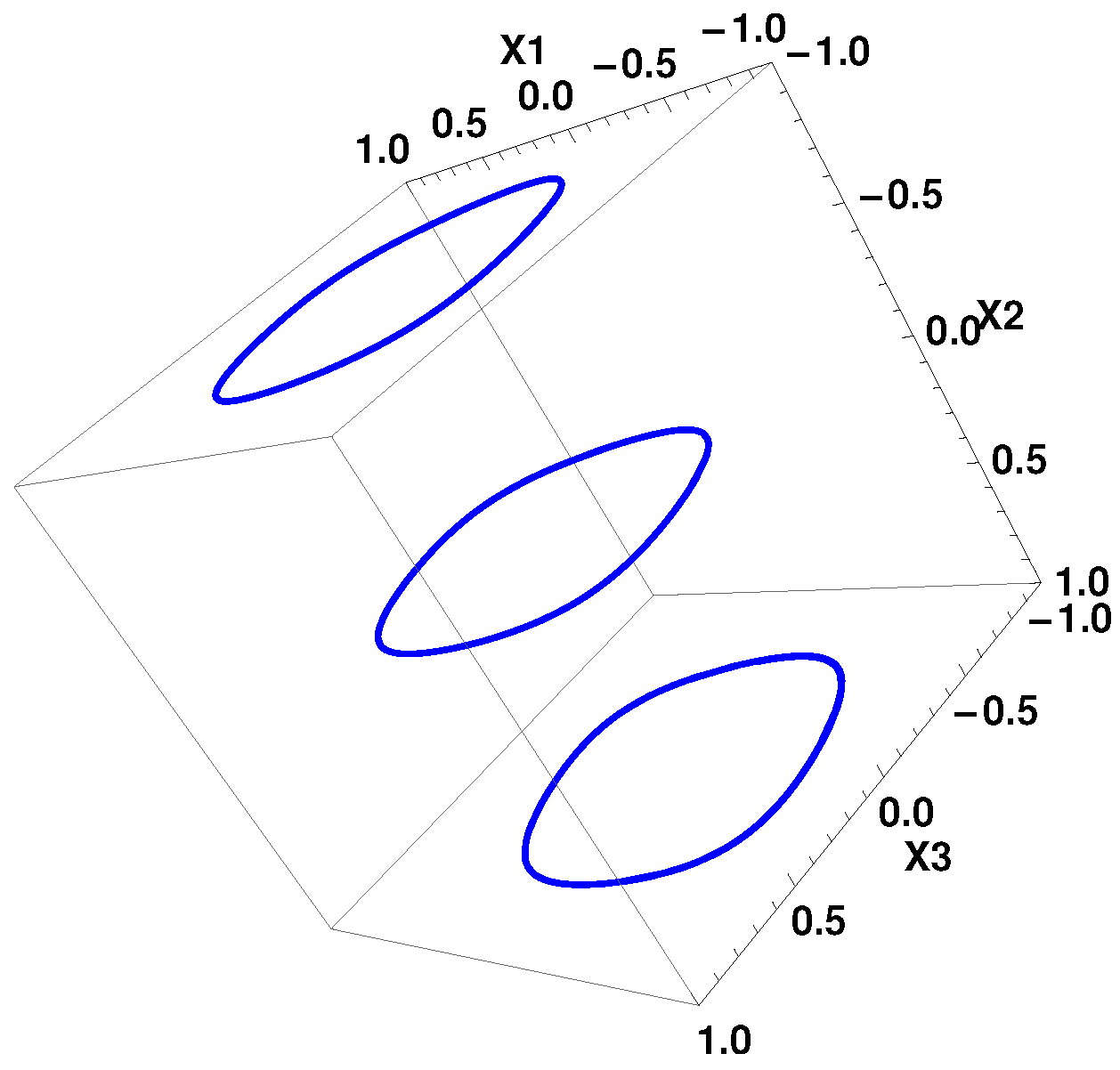
4), which has as attractors three limit cycles. This can be performed via three operations: (1) put the entries of the 2D regulatory matrix, which corresponds to 2D system with the limit cycle L, to the four corners of a 3D matrix A; (2) choose the middle element of the 3D matrix A so, that the equation
with respect to
has exactly three roots
(3) set the four remaining values of
to zero. Set also
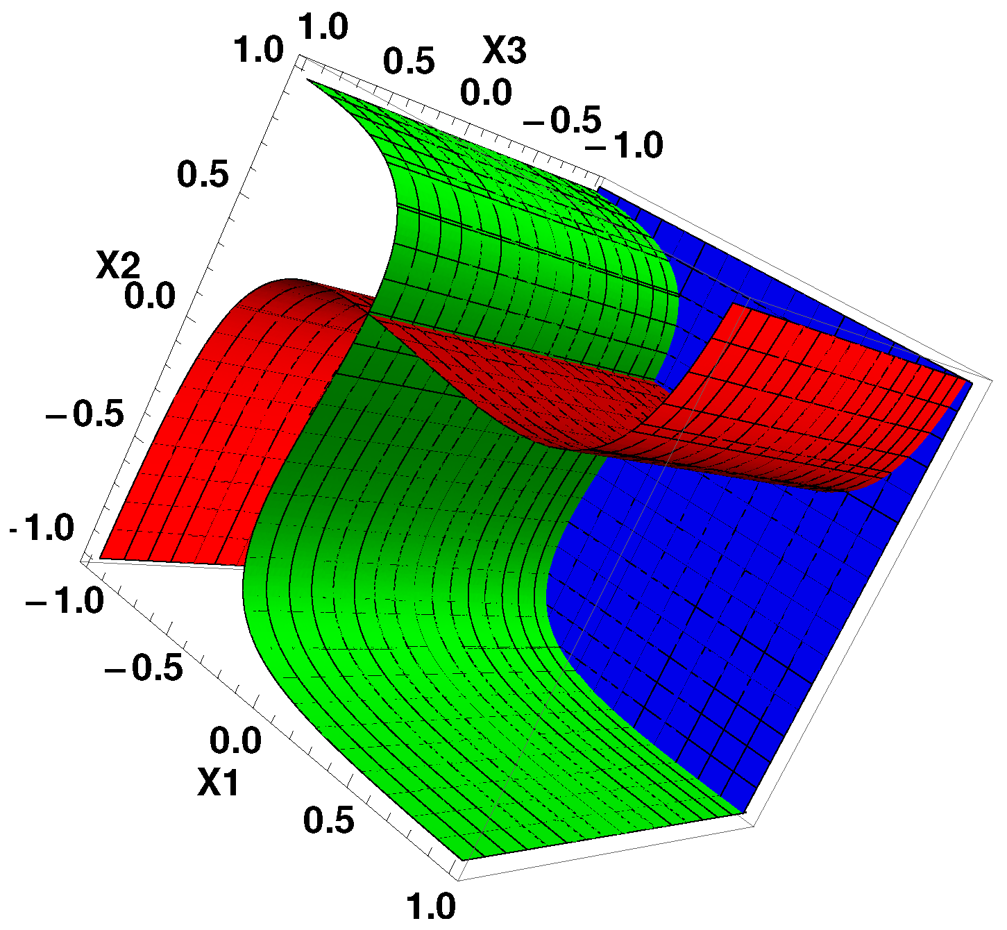
to unity. After finishing these preparations, the second nullcline will be three parallel planes
, going through
Each of these planes will contain the limit cycle. Two side limit cycles will attract trajectories from their neighborhoods. The middle limit cycle will attract only trajectories, lying in the plane
Now, let us solve the problem of control. Let the limit cycle at
be conditionally “bad”. The problem is to change the system so that all trajectories in
are attracted to the limit cycle which, at the beginning of the process, was in the plane
Problems of this kind may arise often. In the paper [
20], a similar problem was treated mathematically for genetic networks.
Solution: Change so that the equation has now the unique root near The second nullcline is now the plane, passing near This operation is possible, since the graph of is sigmoidal, and changing means shifting the original plane in both directions. After that, only one attractor (limit cycle) remains. The problem is solved.
In neuronal systems, the
parameters express the threshold of a response function
f ([
4]). In genetic networks,
stands for the influence of external input on gene
which modulates the gene’s sensitivity of response ([
23]). The technique of changing the
parameters and thus shifting the nullclines was applied in the work [
24] for building the partial control over model of genetic network.


