Impulsive Linearly Implicit Euler Method for the SIR Epidemic Model with Pulse Vaccination Strategy

Abstract

In this paper, a new numerical scheme, which we call the impulsive linearly implicit Euler method, for the SIR epidemic model with pulse vaccination strategy is constructed based on the linearly implicit Euler method. The sufficient conditions for global attractivity of an infection-free periodic solution of the impulsive linearly implicit Euler method are obtained. We further show that the limit of the disease-free periodic solution of the impulsive linearly implicit Euler method is the disease-free periodic solution of the exact solution when the step size tends to 0. Finally, two numerical experiments are given to confirm the conclusions.

1. Introduction

Infectious diseases pose a serious threat to human health and hamper socio-economic development. As early as 1927, Kermack and McKendrick studied the epidemiological processes of the London Black Death and the Bombay Plague and creatively proposed the SIR model [1]. The SIR infections disease model is an important model that has widely been applied to study various infectious diseases such as smallpox, influenza, hepatitis and measles [2,3,4]. Pulse vaccination, the repeated application of a vaccine over a defined age range, is gradually obtaining widespread attention as a strategy for the reduction or eradication of childhood viral infections such as measles and polio. The theoretical work by Agur et al. in the paper [5] laid down some formal ground rules for the mechanism of action of pulse vaccination. The basis of their argument is to repeat pulse vaccination to maintain $R_0$ below unity and then infection is eliminated. Shulgin, Stone and Agur [6] have shown that under a planned pulse vaccination regime, the SIR model with a constant total population converges to a stable solution with the number of infectious individuals equal to zero. Most of the results of the previous research are about the exact solutions of impulsive epidemic equations [7,8,9,10,11,12,13,14]. But, in general, impulsive SIR differential equations cannot be solved exactly or the solving is complicated. So, it is a good choice to study numerical methods for the impulsive SIR equations.

In recent years, more and more experts and scholars have paid attention to the field of the linearly implicit Euler method for SIR equations without impulsive perturbations. In 1992 in [15], a fully-discretized linearly implicit Euler (IMEX) method was proposed for a threshold of numerical methods for an aged SIS model with a finite maximum age, in which some numerical basic reproduction numbers were provided and the stability of the disease-free equilibrium was discussed by the theory of a finite-dimensional sublinear discrete dynamical system. In [16], a numerical reproduction number of the linearly implicit Euler–Riemann method for a single nonlinear age-structured population model with infinite age was studied. A numerical threshold of a linearly implicit Euler method for a nonlinear infection-age SIR model was studied in [17]. It was also shown that the method shares the equilibrium and basic reproduction number $R_0$ of age-independent SIR models for any step size. In [18], the linearly implicit Euler method was applied to numerical representations of global epidemic threshold for nonlinear infection-age SIR models. But to the best of our knowledge, there are no results for applying the linearly implicit Euler method to solve impulsive SIR equations.

The most significant and obvious advantage of the linear implicit Euler method is its ability to maintain the property that the exact solution of the infectious disease model is positive for arbitrary step size, which is an important property in the biological sense. Thus, our first concern is whether the impulsive linear implicit Euler method (ILIEM) can preserve the property that the exact solution of the impulsive SIR equation is positive for arbitrary step size. Pulse vaccination, the repeated application of vaccine over a defined age range, is an important strategy for the elimination of childhood viral infectious such as measles and poliomyelitis [5,6]. In the paper [6], Shulgin, Stone and Agur applied linearized methods combined with the Floquet theory to study the local stability of disease-free periodic solutions. In our present article, we will further investigate the global attractiveness of the disease-free periodic solution of the impulsive SIR system. Another very important and interesting question is whether ILIEM can preserve the global attractiveness of the disease-free periodic solutions of impulsive SIR systems.

The rest of this paper is organized as follows: In Section 2, in order to point out that the ILIEM can preserve some of the properties of the exact solution of the impulsive SIR system, we introduce the following two properties of the impulsive SIR system. First, the exact solution of the impulsive SIR equation is positive when the initial values are positive. Second, the global attractiveness of the disease-free periodic solution of impulsive SIR system is introduced. In Section 3, we first point out the advantages of ILIEM: compared to the impulsive explicit Euler method and the implicit Euler method, the numerical solutions of ILIEM are positive for arbitrary step size $h>0$ when the initial values are positive, and the fact that the computational cost of ILIEM is almost the same as the explicit Euler method. After that, we provide sufficient conditions for the disease-free periodic solution of ILIEM to be globally attractive. Moreover, the limit of the disease-free periodic solution of ILIEM is the disease-free periodic solution of impulsive SIR system when the step size h tends to 0. Finally, in Section 4, two numerical experiments are given to illuminate the correctness of the conclusions.

2. The Exact Solution of Impulsive SIR

In this paper, we will further investigate the following classical impulsive SIR equations which were proposed by Shulgin, Stone and Agur in the paper [6] for measles models

$$\left\{\begin{array}{l}\left.\begin{array}{l}{\displaystyle \frac{dS\left(t\right)}{dt}}=b-\beta S\left(t\right)I\left(t\right)-bS\left(t\right),\\ {\displaystyle \frac{dI\left(t\right)}{dt}}=\beta S\left(t\right)I\left(t\right)-\gamma I\left(t\right)-bI\left(t\right),\\ {\displaystyle \frac{dR\left(t\right)}{dt}}=\gamma I\left(t\right)-bR\left(t\right),\end{array}\right\}t\ne k\tau ,\\ \left.\begin{array}{l}S\left(k{\tau }^{+}\right)=(1-p)S\left(k\tau \right),\\ I\left(k{\tau }^{+}\right)=I\left(k\tau \right),\\ R\left(k{\tau }^{+}\right)=pS\left(k\tau \right)+R\left(k\tau \right),\end{array}\right\}t=k\tau ,\\ S\left(0^{+}\right)=S_0,I\left(0^{+}\right)=I_0,R\left(0^{+}\right)=R_0,\end{array}\right.$$

(1)

where $\tau$ is a positive real constant, $k\in {\mathbb{Z}}^{+}=\{1,2,\cdots \}$, S, I and R are the proportion of individuals susceptible, infected and recovered to the disease, respectively. b denotes the birth rate and b also denotes the death rate, $\gamma$ is the recovery rate. Susceptibles become infectious at a rate $\beta I$, which $\beta$ is the contact rate. The pulse vaccination scheme proposes to vaccinate a fraction p of the entire susceptible population in a single pulse, applied every $\tau$ years and that p satisfies $0<p<1$. $S_0$, $I_0$ and $R_0$ are nonnegative initial values, and satisfy $S_0+I_0+R_0=1$. From this combination with Equation (1), we can easily prove that the following equality

$$S\left(t\right)+I\left(t\right)+R\left(t\right)\equiv 1$$

holds for all t. So, we need only consider the following impulsive system

$$\left\{\begin{array}{l}\left.\begin{array}{l}{\displaystyle \frac{dS\left(t\right)}{dt}}=b-\beta S\left(t\right)I\left(t\right)-bS\left(t\right),\\ {\displaystyle \frac{dI\left(t\right)}{dt}}=\beta S\left(t\right)I\left(t\right)-\gamma I\left(t\right)-bI\left(t\right),\end{array}\right\}t\ne k\tau ,\\ \left.\begin{array}{l}S\left(k{\tau }^{+}\right)=(1-p)S\left(k\tau \right),\\ I\left(k{\tau }^{+}\right)=I\left(k\tau \right),\end{array}\right\}t=k\tau ,\end{array}\right.$$

(2)

with initial values $S\left(0^{+}\right)=S_0$ and $I\left(0^{+}\right)=I_0$. It is easy to see that model (2) is invariant in the set

$$\Omega =\left\{\right(S,I):0\le S\le 1,0\le I\le 1,S+I\le 1\}.$$

When $I=0$, $S\left(t\right)$ in (2) satisfies the following system

$$\left\{\begin{array}{cc}{\displaystyle \frac{dS\left(t\right)}{dt}}=b-bS\left(t\right),\hfill & t\ne n\tau ,\hfill \\ S\left(n{\tau }^{+}\right)=(1-p)S\left(n\tau \right),\hfill & t=n\tau .\hfill \end{array}\right.$$

(3)

From paper [6], we know that the Equation (3) has the following globally asymptotically stable periodic solution

$$\tilde{S}\left(t\right)=1-(1-S^{\ast }){\mathrm{e}}^{-b(t-k\tau )},t\in (k\tau ,(k+1)\tau ],$$

(4)

where $S^{\ast }={\displaystyle \frac{(1-p)(1-{\mathrm{e}}^{-b\tau })}{1-(1-p){\mathrm{e}}^{-b\tau }}}$.

Theorem 1.

If $\sigma <1$, then the infection-free periodic solution $(\tilde{S}\left(t\right),0)$ in system (2) is globally attractive, where

$$\sigma ={\displaystyle \frac{\beta (1-{\mathrm{e}}^{-b\tau })}{(b+\gamma )\left(1-(1-p){\mathrm{e}}^{-b\tau }\right)}}.$$

(5)

Proof. 

Since $\sigma <1$, we can choose ${ϵ}_1>0$ to be sufficiently small such that

$$\beta \left({\displaystyle \frac{(1-{\mathrm{e}}^{-b\tau })}{1-(1-p){\mathrm{e}}^{-b\tau }}}+{ϵ}_1\right)<b+\gamma .$$

(6)

From the first equation of (2), we obtain ${\displaystyle \frac{dS\left(t\right)}{dt}}\le b-bS\left(t\right)$. Then, we consider the comparison system with pulses

$$\left\{\begin{array}{cc}{\displaystyle \frac{dx\left(t\right)}{dt}}=b-bx\left(t\right),\hfill & t\ne k\tau ,\hfill \\ x\left(k{\tau }^{+}\right)=(1-p)x\left(k\tau \right),\hfill & t=k\tau .\hfill \end{array}\right.$$

(7)

By similar discussions as above, there exists a unique periodic solution $\tilde{x}\left(t\right)=\tilde{S}\left(t\right)$ of system (7), which is globally asymptotically stable.

Let $\left(S\right(t),I(t\left)\right)$ be the solution of the impulsive Equation (2) with initial condition $S\left(0^{+}\right)=S_0>0$. With the comparison theorem for impulsive equations [19,20], there exists an integer $k_1>0$ such that

$$S\left(t\right)<\tilde{S}\left(t\right)+{ϵ}_1\le {\displaystyle \frac{1-{\mathrm{e}}^{-b\tau }}{1-(1-p){\mathrm{e}}^{-b\tau }}}+{ϵ}_1=\delta ,k\tau <t\le (k+1)\tau ,k>k_1,$$

(8)

where $\tilde{S}\left(t\right)$ is defined in (4). Further, from the second equation of (2), we know that (8) implies

$${\displaystyle \frac{dI\left(t\right)}{dt}}\le (\beta \delta -\gamma -b)I\left(t\right),k>k_1.$$

Consider the following comparison system

$${\displaystyle \frac{dy\left(t\right)}{dt}}=(\beta \delta -\gamma -b)y\left(t\right).$$

By the expression of (6), we have $\beta \delta -\gamma -b<0$. It is easy to see that $\underset{t\to +\infty }{lim}y\left(t\right)=0$. By the comparison theorem [21,22], we have $\underset{t\to +\infty }{lim\; sup}I\left(t\right)\le \underset{t\to +\infty }{lim\; sup}y\left(t\right)=0$. Incorporating into the positive of $I\left(t\right)$, we know that $\underset{t\to +\infty }{lim}I\left(t\right)=0$. Consequently, there exists an integer $k_2>k_1$ such that $I\left(t\right)<{ϵ}_1$ for all $t>k_2\tau$. For the first equation of (2), we can obtain

$${\displaystyle \frac{dS\left(t\right)}{dt}}\ge b-(\beta {ϵ}_1+b)S\left(t\right).$$

Consider comparison impulsive differential equations for $t>k_2\tau$ and $k>k_2$,

$$\left\{\begin{array}{cc}{\displaystyle \frac{dz\left(t\right)}{dt}}=b-(\beta {ϵ}_1+b)z\left(t\right),\hfill & t\ne k\tau ,\hfill \\ z\left(k{\tau }^{+}\right)=(1-p)z\left(k\tau \right),\hfill & t=k\tau .\hfill \end{array}\right.$$

(9)

By [9] (Lemma 2.2) or [10] (Lemma 2.1), we have the periodic solution of (9),

$$\tilde{z}\left(t\right)={\displaystyle \frac{b}{\beta {ϵ}_1+b}}-({\displaystyle \frac{b}{\beta {ϵ}_1+b}}-z^{\ast }){\mathrm{e}}^{-(\beta {ϵ}_1+b)(t-k\tau )},k\tau <t\le (k+1)\tau ,k>k_2,$$

where $z^{\ast }={\displaystyle \frac{b(1-p)\left(1-{\mathrm{e}}^{-(\beta {ϵ}_1+b)\tau }\right)}{(\beta {ϵ}_1+b)\left(1-(1-p){\mathrm{e}}^{-(\beta {ϵ}_1+b)\tau }\right)}}$. According to the comparison theorem for impulsive differential equations [19,20], there exists an integer $k_3>k_2$ such that

$$S\left(t\right)>\tilde{z}\left(t\right)-{ϵ}_1,k\tau <t\le (k+1)\tau ,k>k_3,$$

(10)

Because ${ϵ}_1$ is arbitrarily small, it follows from (8) and (10) that

$$\tilde{S}\left(t\right)=1-{\displaystyle \frac{p{\mathrm{e}}^{-b(t-k\tau )}}{1-(1-p){\mathrm{e}}^{-b\tau }}},t\in (k\tau ,(k+1)\tau ],$$

is globally attractive. Therefore, the infection-free solution $(\tilde{S}\left(t\right),0)$ is globally attractive. □

3. ILIEM for Impulsive SIR

The ILIEM for (1) can be constructed as follows

$$\left\{\begin{array}{cc}{S}_{k,l+1}=S_{k,l}+h\left(b-\beta S_{k,l+1}{I}_{k,l}-b{S}_{k,l+1}\right),\hfill & k\in \mathbb{N},\hfill \\ I_{k,l+1}=I_{k,l}+h\left(\beta S_{k,l+1}{I}_{k,l}-\gamma I_{k,l+1}-b{I}_{k,l+1}\right),\hfill & l\in \mathbb{A},\hfill \\ R_{k,l+1}=R_{k,l}+h\left(\gamma I_{k,l+1}-b{R}_{k,l+1}\right),\hfill & \\ S_{k+1,0}=(1-p)S_{k,m},\hfill & \\ I_{k+1,0}=I_{k,m},\hfill & \\ R_{k+1,0}=p{S}_{k,m}+R_{k,m},\hfill & \\ S_{0,0}=S_0,I_{0,0}=I_0,R_{0,0}=R_0,\hfill \end{array}\right.$$

(11)

where the step size $h={\displaystyle \frac{\tau }{m}}$, m is a positive constant, and $\mathbb{N}=\{0,1,2,\cdots \}$. Conveniently, denote ${\mathbb{Z}}^{+}=\{1,2,\cdots \}$, $\mathbb{A}=\{0,1,2,\cdots ,m-1\}$ and $\mathbb{B}=\{0,1,2,\cdots ,m\}$. Let $t_{k,l}$ be the sequence of discretization nodes, where $t_{k,l}=(km+l)h=k\tau +lh$, $k\in \mathbb{N}$,$l\in \mathbb{B}$ and $t_{k,m}=t_{k+1,0}=k\tau$, $k\in {\mathbb{Z}}^{+}$. The exact solutions $S\left(t_{k,l}\right)$, $I\left(t_{k,l}\right)$ and $R\left(t_{k,l}\right)$ ($k\in \mathbb{N}$, $l\in \mathbb{B}-\left\{0\right\}$) will be approximated by $S_{k,l}$, $I_{k,l}$ and $R_{k,l}$, respectively. Simultaneously, $S\left(k{\tau }^{+}\right)$, $I\left(k{\tau }^{+}\right)$ and $R\left(k{\tau }^{+}\right)$ ($k\in \mathbb{N}$) will be approximated by $S_{k,0}$, $I_{k,0}$ and $R_{k,0}$, respectively.

3.1. Advantages of ILIELM

The impulsive explicit Euler method [23] for (1) can be constructed as follows

$$\left\{\begin{array}{cc}{S}_{k,l+1}=S_{k,l}+h\left(b-\beta S_{k,l}{I}_{k,l}-b{S}_{k,l}\right),\hfill & k\in \mathbb{N},\hfill \\ I_{k,l+1}=I_{k,l}+h\left(\beta S_{k,l}{I}_{k,l}-\gamma I_{k,l}-b{I}_{k,l}\right),\hfill & l\in \mathbb{A},\hfill \\ R_{k,l+1}=R_{k,l}+h\left(\gamma I_{k,l}-b{R}_{k,l}\right),\hfill & \\ S_{k+1,0}=(1-p)S_{k,m},\hfill & \\ I_{k+1,0}=I_{k,m},\hfill & \\ R_{k+1,0}=p{S}_{k,m}+R_{k,m},\hfill & \\ S_{0,0}=S_0,I_{0,0}=I_0,R_{0,0}=R_0.\hfill \end{array}\right.$$

This is a numerical method of calculation with high efficiency but $S_{k,l+1}=hb+\left(1-h\beta I_{k,l}\right.\left.-hb\right)S_{k,l}$ is possibly negative for some large $I_{k,l}>0$.

Similarly, the impulsive implicit Euler method [23] for (1) can be constructed as follows

$$\left\{\begin{array}{cc}{S}_{k,l+1}=S_{k,l}+h\left(b-\beta S_{k,l+1}{I}_{k,l+1}-b{S}_{k,l+1}\right),\hfill & k\in \mathbb{N},\hfill \\ I_{k,l+1}=I_{k,l}+h\left(\beta S_{k,l+1}{I}_{k,l+1}-\gamma I_{k,l+1}-b{I}_{k,l+1}\right),\hfill & l\in \mathbb{A},\hfill \\ R_{k,l+1}=R_{k,l}+h\left(\gamma I_{k,l+1}-b{R}_{k,l+1}\right),\hfill & \\ S_{k+1,0}=(1-p)S_{k,m},\hfill & \\ I_{k+1,0}=I_{k,m},\hfill & \\ R_{k+1,0}=p{S}_{k,m}+R_{k,m},\hfill & \\ S_{0,0}=S_0,I_{0,0}=I_0,R_{0,0}=R_0.\hfill \end{array}\right.$$

Hence, besides the computational cost, $I_{k,l+1}={(1-h\beta S_{k,l+1}+h\gamma +hb)}^{-1}{I}_{k,l}$ is possibly negative for some large $S_{k,l+1}>0$.

Obviously, ILIELM (11) can be rewritten as

$$\left\{\begin{array}{cc}{S}_{k,l+1}={\displaystyle \frac{S_{k,l}+hb}{1+h\beta I_{k,l}+hb}},\hfill & k\in \mathbb{N},\hfill \\ I_{k,l+1}={\displaystyle \frac{I_{k,l}+h\beta S_{k,l+1}{I}_{k,l}}{1+h\gamma +hb}},\hfill & l\in \mathbb{A},\hfill \\ R_{k,l+1}={\displaystyle \frac{R_{k,l}+h\gamma I_{k,l+1}}{1+hb}},\hfill & \\ S_{k+1,0}=(1-p)S_{k,m},\hfill & \\ I_{k+1,0}=I_{k,m},\hfill & \\ R_{k+1,0}=p{S}_{k,m}+R_{k,m},\hfill & \\ S_{0,0}=S_0,I_{0,0}=I_0,R_{0,0}=R_0.\hfill \end{array}\right.$$

(12)

From the expression of (12), we can see that the computational cost is almost the same as impulsive explicit Euler method. From the expression of (12), we can also obtain the following theorem:

Theorem 2.

Any solution $(S_{k,l},I_{k,l},R_{k,l})$ of the system (11) is positive for any h and all $k\in \mathbb{N}$, $l\in \mathbb{B}$, when the initial values’ vector $(S_0,I_0,R_0)$ is positive.

Theorem 3.

For any solution $(S_{k,l},I_{k,l},R_{k,l})$ of the system (11), the total number $N_{k,l}=S_{k,l}+I_{k,l}+R_{k,l}$ satisfies $N_{k,l}\equiv 1$, $\forall k\in \mathbb{N},\forall l\in \mathbb{B}$, if $N_{0,0}=S_{0,0}+I_{0,0}+R_{0,0}=1$.

Proof. 

By the first three equations of (11), we can obtain that

$$N_{k,l+1}={\displaystyle \frac{hb+N_{k,l}}{1+hb}}=1,\forall k\in \mathbb{N},\forall l\in \mathbb{A},$$

under the condition $N_{k,l}=1$. Obviously, by the last three equations of (11), we have

$$N_{k+1,0}=N_{k,m},\forall k\in \mathbb{N}.$$

Applying mathematical induction, we can show that $N_{k,l}=1$, $k\in \mathbb{N}$, $l=0,1,2,\cdots ,m$. The proof has been completed. □

Similar to the previous analysis of the exact solution, we only need to consider the linearly implicit Euler method for (2) as follows

$$\left\{\begin{array}{cc}{S}_{k,l+1}=S_{k,l}+h\left(b-\beta S_{k,l+1}{I}_{k,l}-b{S}_{k,l+1}\right),\hfill & k\in \mathbb{N},\hfill \\ I_{k,l+1}=I_{k,l}+h\left(\beta S_{k,l+1}{I}_{k,l}-\gamma I_{k,l+1}-b{I}_{k,l+1}\right),\hfill & l\in \mathbb{A},\hfill \\ S_{k+1,0}=(1-p)S_{k,m},\hfill & \\ I_{k+1,0}=I_{k,m},\hfill \end{array}\right.$$

(13)

with initial values $S_{0,0}=S_0$, $I_{0,0}=I_0$.

For convenience, we will write [24] (Lemma 5) in the following form:

Lemma 1.

Consider the following impulsive difference equations

$$\left\{\begin{array}{cc}{\omega }_{k,l+1}=\lambda +\mu {\omega }_{k,l},\hfill & k\in \mathbb{N},l\in \mathbb{A},\hfill \\ {\omega }_{k+1,0}=(1-\theta ){\omega }_{k,m},\hfill & k\in \mathbb{N}\hfill \end{array}\right.$$

(14)

where $\lambda >0$, $0<\mu <1$ and $0<\theta <1$. The system (4) has a unique positive periodic solution, for $k\in \mathbb{N},l\in \mathbb{B}$,

$${\tilde{\omega }}_{k,l}={\displaystyle \frac{\lambda \left(1-{\mu }^l\right)}{1-\mu }}+{\displaystyle \frac{{\mu }^l\lambda (1-\theta )(1-{\mu }^m)}{\left(1-\mu \right)\left[1-(1-\theta ){\mu }^m\right]}}$$

(15)

which is globally asymptotically stable.

3.2. Global Attractivity of Disease-Free Periodic Solution of ILIEM

To begin with, we demonstrate the existence of an infection-free periodic solution, in which infectious individuals are entirely absent from population permanently, $I_{k,l}$ for $\forall k\in \mathbb{N}$, $l\in \mathbb{B}$.

$$\left\{\begin{array}{cc}{S}_{k,l+1}=S_{k,l}+hb-hb{S}_{k,l+1},\hfill & \forall k\in \mathbb{N},l\in \mathbb{A},\hfill \\ S_{k+1,0}=(1-p)S_{k,m},\hfill & \forall k\in \mathbb{N},\hfill \end{array}\right.$$

(16)

which can be rewritten as follows

$$\left\{\begin{array}{cc}{S}_{k,l+1}={\displaystyle \frac{hb}{1+hb}}+{\displaystyle \frac{S_{k,l}}{1+hb}},\hfill & \forall k\in \mathbb{N},l\in \mathbb{A},\hfill \\ S_{k+1,0}=(1-p)S_{k,m},\hfill & \forall k\in \mathbb{N}.\hfill \end{array}\right.$$

By Lemma 1, it is easy to obtain the periodic solution system (16) as follows

$${\tilde{S}}_{k,l}=1-{(1+hb)}^{-l}+{\displaystyle \frac{{(1+hb)}^{-l}(1-p)\left[1-{(1+hb)}^{-m}\right]}{1-(1-p){(1+hb)}^{-m}}}.$$

(17)

Theorem 4.

If ${\sigma }_d<1$, then the disease-free periodic solution $({\tilde{S}}_{k,l},0)$ of ILIEM (13) is globally attractive, where

$${\sigma }_d={\displaystyle \frac{1}{(1+h\gamma +hb)}}\left(1+{\displaystyle \frac{h\beta \left(1-{(1+hb)}^{-m}\right)}{1-(1-p){(1+hb)}^{-m}}}\right).$$

Proof. 

By the first equation of (12), we can obtain that

$$S_{k,l+1}={\displaystyle \frac{S_{k,l}+hb}{1+hb+h\beta I_{k,l}}}\le {\displaystyle \frac{S_{k,l}+hb}{1+hb}}.$$

Next, we consider the following comparison system with pulse:

$$\left\{\begin{array}{cc}{x}_{k,l+1}={\displaystyle \frac{hb}{1+hb}}+{\displaystyle \frac{x_{k,l}}{1+hb}},\hfill & k\in \mathbb{N},l\in \mathbb{A},\hfill \\ x_{k+1,0}=(1-p)x_{k,m},\hfill & k\in \mathbb{N}.\hfill \end{array}\right.$$

Applying Lemma 1, we can obtain the following periodic solution

$${\tilde{x}}_{k,l}=1-{(1+hb)}^{-l}+{\displaystyle \frac{{(1+hb)}^{-l}(1-p)\left[1-{(1+hb)}^{-m}\right]}{1-(1-p){(1+hb)}^{-m}}}.$$

By the non-negativity of $S_{k,l}$ and $x_{k,l}$, there exists an integer $N_1\in {\mathbb{Z}}^{+}$ such that

$$S_{k,l}\le x_{k,l}<{\tilde{x}}_{k,l}+{ϵ}_1,\forall k\ge N_1,\forall l\in \mathbb{B}.$$

Hence, we have

$$S_{k,l}\le {\displaystyle \frac{1-{(1+hb)}^{-m}}{1-(1-p){(1+hb)}^{-m}}}+{ϵ}_1=S_d^{\ast }.$$

Further, from the second equation of (12), we can obtain that

$$\left|I_{k,l+1}\right|=\left|{\displaystyle \frac{I_{k,l}+h\beta S_{k,l+1}{I}_{k,l}}{1+h\gamma +hb}}\right|\le \left|{\displaystyle \frac{1+h\beta S_d^{\ast }}{1+h\gamma +hb}}\right|·\left|I_{k,l}\right|.$$

Obviously, ${\sigma }_d<1$ implies that

$$\left|{\displaystyle \frac{1+h\beta S_d^{\ast }}{1+h\gamma +hb}}\right|<1.$$

Consequently, we have $\underset{k\to +\infty }{lim}{I}_{k,l}=0$, $\forall l\in \mathbb{B}$. For any small ${ϵ}_2>0$, there exists an integer $N_2$ such that $|I_{k,l}|<{ϵ}_2$, $k\ge N_2$. Hence, by the first equation of (12), we can obtain that

$$S_{k,l+1}={\displaystyle \frac{S_{k,l}+hb}{1+hb+h\beta I_{k,l}}}\ge {\displaystyle \frac{S_{k,l}+hb}{1+hb+h\beta {ϵ}_2}}.$$

Next, we consider the following comparison system with pulse:

$$\left\{\begin{array}{cc}{y}_{k,l+1}={\displaystyle \frac{hb}{1+hb+h\beta {ϵ}_2}}+{\displaystyle \frac{y_{k,l}}{1+hb+h\beta {ϵ}_2}},\hfill & k\in \mathbb{N},l\in \mathbb{A},\hfill \\ y_{k+1,0}=(1-p)y_{k,m},\hfill & k\in \mathbb{N}.\hfill \end{array}\right.$$

Applying Lemma 1, we can obtain the following periodic solution

$${\tilde{y}}_{k,l}={\displaystyle \frac{b}{b+\beta {ϵ}_2}}\left(1-{\displaystyle \frac{p}{{(1+hb+h\beta {ϵ}_2)}^l}}·{\displaystyle \frac{1}{1-\frac{1-p}{{(1+hb+h\beta {ϵ}_2)}^m}}}\right).$$

By the non-negativity of $S_{k,l}$ and $y_{k,l}$, there exists an integer $N_2\in {\mathbb{Z}}^{+}$ such that

$$S_{k,l}\ge y_{k,l}>{\tilde{y}}_{k,l}-{ϵ}_2,\forall k\ge N_2,\forall l\in \mathbb{B}.$$

Since ${ϵ}_1$ and ${ϵ}_2$ are sufficiently small, ${\tilde{S}}_{k,l}$ is globally attractive. Similarly, we show that ${\tilde{R}}_{k,l}$ is also globally attractive. Consequently, the infection-free periodic solution $({\tilde{S}}_{k,l},0)$ is also globally attractive. □

Theorem 1 shows that the disease-free periodic solution of impulsive system (2) is globally attractive under the condition $\sigma <1$. The following result will show that under the same condition, the disease-free periodic solution the disease-free periodic solution of ILIEM (13) is also globally attractive when $hb<1$.

Corollary 1.

If $\sigma <1$, then the disease-free periodic solution $({\tilde{S}}_{k,l},0)$ of ILIEM (13) is globally attractive; arbitrary h satisfies $hb<1$.

Proof. 

Let the function

$$f\left(x\right)={\displaystyle \frac{\beta (1-x)}{1-(1-p)x}},0\le x\le 1.$$

Taking the derivative gives

$$f\prime \left(x\right)={\displaystyle \frac{-p\beta }{{\left(1-(1-p)x\right)}^2}}<0,$$

which means that $f\left(x\right)$ is monotonically decreasing on $[0,1]$. Since ${(1+hb)}^{{\displaystyle \frac{1}{hb}}}<\mathrm{e}$ holds for $0<hb<1$, we have

$${(1+hb)}^{-m}>{\mathrm{e}}^{-bhm}={\mathrm{e}}^{-b\tau },$$

which implies that

$$f\left({(1+hb)}^{-m}\right)<f\left({\mathrm{e}}^{-b\tau }\right),$$

that is

$${\displaystyle \frac{\beta (1-{(1+hb)}^{-m})}{1-(1-p){(1+hb)}^{-m}}}<{\displaystyle \frac{\beta (1-{\mathrm{e}}^{-b\tau })}{1-(1-p){\mathrm{e}}^{-b\tau }}}.$$

Consequently, we have

$$\begin{array}{ccc}& & \sigma <1\hfill \\ & \Rightarrow & {\displaystyle \frac{\beta (1-{\mathrm{e}}^{-b\tau })}{1-(1-p){\mathrm{e}}^{-b\tau }}}<b+\gamma \hfill \\ & \Rightarrow & {\displaystyle \frac{\beta (1-{(1+hb)}^{-m})}{1-(1-p){(1+hb)}^{-m}}}<b+\gamma \hfill \\ & \Rightarrow & {\sigma }_d<1.\hfill \end{array}$$

Applying Theorem 4, the infection-free periodic $({\tilde{S}}_{k,l},0)$ is globally attractive and arbitrary h satisfies $hb<1$. The proof is completed. □

Theorem 5.

The limit of the discrete disease-free periodic solution $({\tilde{S}}_{k,l},0)$ of ILIEM (13) is the disease-free periodic solution $(\tilde{S}\left(t\right),0)$ of impulsive SIR (2) when the step size h tends 0. In the following sense, for any moment fixed at t, there exists a nonnegative integer k such that $t\in (k\tau ,(k+1\left)\tau \right]$ and

$$\underset{h\to 0,mh=\tau ,t=(km+l)h}{lim}({\tilde{S}}_{k,l},0)=(\tilde{S}\left(t\right),0).$$

Proof. 

Obviously, we have

$$\underset{h\to 0,mh=\tau ,t=(km+l)h}{lim}{(1+hb)}^{-l}=\underset{h\to 0,mh=\tau ,t=(km+l)h}{lim}{(1+hb)}^{{\displaystyle \frac{1}{hb}}(-hlb)}={\mathrm{e}}^{-b(t-k\tau )}.$$

and

$$\underset{h\to 0,mh=\tau }{lim}{(1+hb)}^{-m}=\underset{h\to 0,mh=\tau }{lim}{(1+hb)}^{{\displaystyle \frac{1}{hb}}(-hmb)}={\mathrm{e}}^{-b\tau }.$$

Combining the above two equalities with (4) and (17), we can obtain

$$\begin{array}{ccc}& & \underset{h\to 0,mh=\tau ,t=(km+l)h}{lim}{\tilde{S}}_{k,l}\hfill \\ & =& \underset{h\to 0,mh=\tau ,t=(km+l)h}{lim}\left(1-{(1+hb)}^{-l}+{\displaystyle \frac{{(1+hb)}^{-l}(1-p)\left(1-{(1+hb)}^{-m}\right)}{1-(1-p){(1+hb)}^{-m}}}\right)\hfill \\ & =& 1-{\mathrm{e}}^{-b(t-k\tau )}+{\displaystyle \frac{{\mathrm{e}}^{-b(t-kT)}(1-p)\left(1-{\mathrm{e}}^{-b\tau }\right)}{1-(1-p){\mathrm{e}}^{-b\tau }}}\hfill \\ & =& \tilde{S}\left(t\right).\hfill \end{array}$$

The proof is completed. □

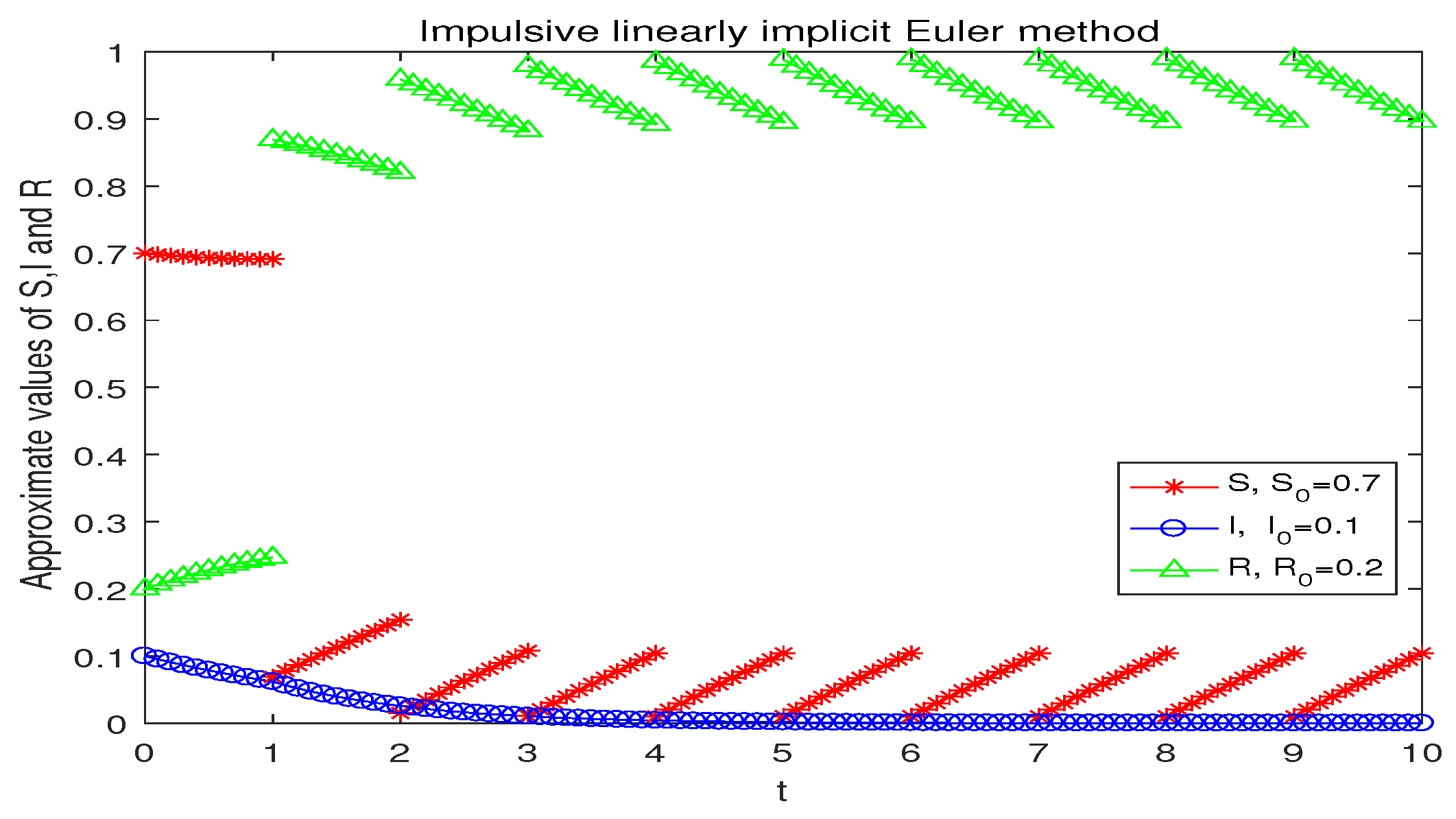
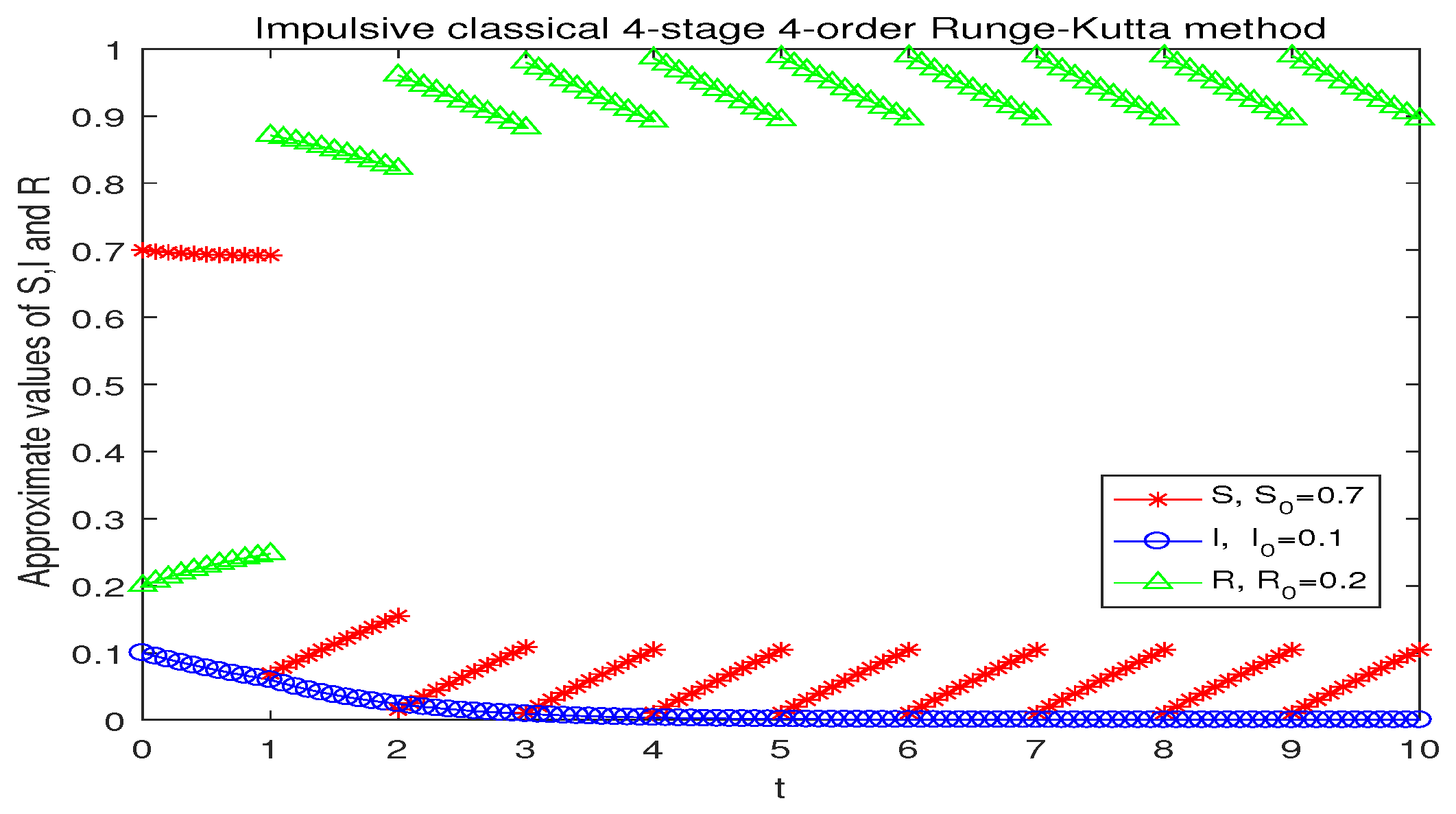
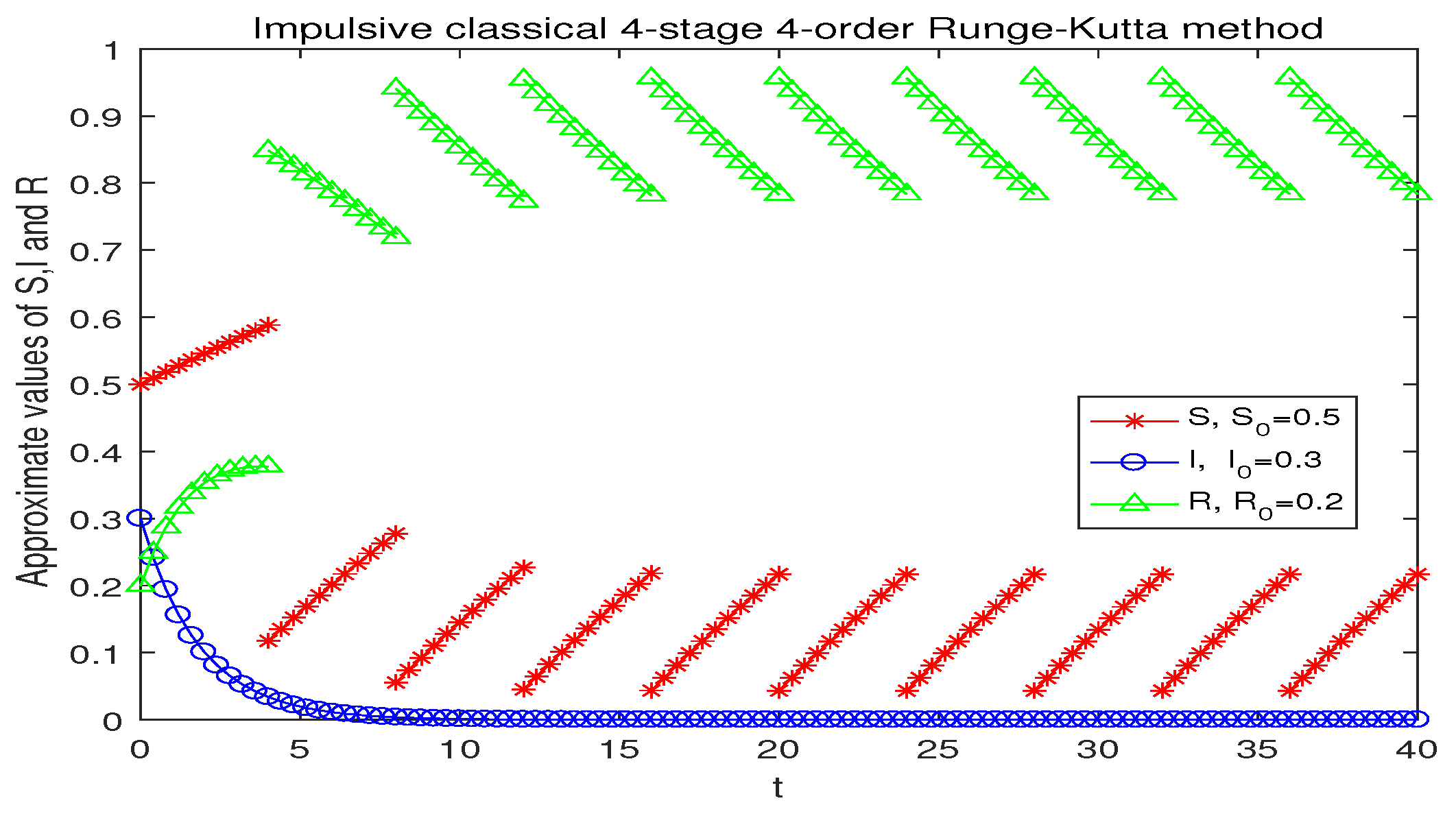
4. Numerical Experiments

From the papers [5,6], we know that the basic reproductive rate of an epidemic is

$$R_0={\displaystyle \frac{\beta }{(b+\gamma )\tau }}\underset{0}{\overset{\tau }{\int }}\tilde{S}\left(t\right)dt.$$

Moreover, $R_0<1$, which is equivalent to ${\displaystyle \frac{1}{\tau }}\underset{0}{\overset{\tau }{\int }}\tilde{S}\left(t\right)dt<{\displaystyle \frac{b+\gamma }{\beta }}=S_c$, implies the disease-free periodic solution $(\tilde{S}\left(t\right),0)$ in system (2) is locally stable. The condition $\sigma <1$ in our present article to ensure that the disease-free periodic solution $(\tilde{S}\left(t\right),0)$ in system (2) is globally attractive, which is equivalent to $\tilde{S}\left(t\right)<S_c$, implies $R_0<1$. In reality, pulse vaccination is an important strategy for the elimination of childhood viral infections such as measles and poliomyelitis [5,6]. Infectious diseases can be controlled by reducing the vaccination interval $\tau$ and increasing the vaccination rate p. It is easy to see in our paper that the condition $\sigma <1$ can be satisfied by controlling the parameters $\tau$ and p. The condition $\sigma <1$ is not a very stringent condition. The following two examples fulfil this condition and we will use them to illustrate the correctness of the theory obtained in this paper.

Example 1.

Consider the impulsive SIR model (1) as $b=0.1$, $\beta =0.7$, $\gamma =0.6$, $p=0.9$ and $\tau =1$ (see Figure 1 and Figure 2). By (5), it is easy to work out that $\sigma \approx 0.073<1$. By Theorem 1, the infection-free periodic solution $(\tilde{S}\left(t\right),0)$ in system (2) is globally attractive, where

$$\tilde{S}\left(t\right)=1-{\displaystyle \frac{0.9{\mathrm{e}}^{-0.1(t-k)}}{1-0.1{\mathrm{e}}^{-0.1}}},t\in (k,k+1],\forall k\in \mathbb{N}.$$

(18)

Applying Corollary 1, the infection-free periodic $({\tilde{S}}_{k,l},0)$ is globally attractive; for arbitrary $h={\displaystyle \frac{1}{m}}$, m is an integer, where

$${\tilde{S}}_{k,l}=1-{\displaystyle \frac{0.9{(1+0.1h)}^{-l}}{1-0.1{(1+0.1h)}^{-m}}},\forall k\in \mathbb{N},l\in \mathbb{B}.$$

(19)

From (18) and (19), we can see that for arbitrary fixed t,

$$\underset{h\to 0,mh=1,t=(km+l)h}{lim}{\tilde{S}}_{k,l}=\tilde{S}\left(t\right),$$

which verifies the correctness of Theorem 5.

The reason we can hardly see the difference between Figure 1 and Figure 2, as well between Figure 3 and Figure 4, with the naked eye is that when the step size is small, the errors between the numerical solution and the exact solution for both numerical methods are very small. We can also see this from

Table 1. The global errors of numerical methods for (1) at the time $t=5$ when $b=0.1$, $\beta =0.7$, $\gamma =0.6$, $p=0.9$ and $\tau =1$.

h	ILIEM	IEEM	IIEM	ICRKM
0.1	6.57948689 × ${10}^{-4}$	6.30555457 × ${10}^{-4}$	6.26634906 × ${10}^{-4}$	5.37914547 × ${10}^{-9}$
0.05	3.27534435 × ${10}^{-4}$	3.14709001 × ${10}^{-4}$	3.13734221 × ${10}^{-4}$	3.28104266 × ${10}^{-10}$
0.025	1.63436238 × ${10}^{-4}$	1.57223011 × ${10}^{-4}$	1.56979647 × ${10}^{-4}$	2.05065166 × ${10}^{-11}$
0.0125	8.16423855 × ${10}^{-5}$	7.85798926 × ${10}^{-5}$	7.85190685 × ${10}^{-5}$	1.28165730 × ${10}^{-12}$
Ratio	0.49877817	0.49949288	0.50040328	0.06199036

and

Table 2. The global errors of numerical methods for (1) at the time $t=8$, when $b=0.05$, $\beta =0.01$, $\gamma =0.5$, $p=0.8$, $\tau =4$.

h	ILIEM	IEEM	IIEM	ICRKM
0.4	0.00262953	0.00229213	0.00255089	5.35118642 × ${10}^{-7}$
0.2	0.00128341	0.00117865	0.00124397	3.05181855 × ${10}^{-8}$
0.1	6.33713258 × ${10}^{-4}$	5.97552229 × ${10}^{-4}$	6.13920780 × ${10}^{-4}$	1.81923606 × ${10}^{-9}$
0.05	3.14845822 × ${10}^{-4}$	3.00831601 × ${10}^{-4}$	3.04926145 × ${10}^{-4}$	1.08122410 × ${10}^{-10}$
Ratio	0.49286547	0.50817288	0.49259289	0.05866777

. This also shows that ILIEM is a very applicable numerical method.

Example 2.

Consider the impulsive SIR model (1) as $b=0.05$, $\beta =0.01$, $\gamma =0.5$, $p=0.8$ and $\tau =4$ (see Figure 3 and Figure 4). By (5), it is easy to work out that $\sigma \approx 0.0039<1$. By Theorem 1, the infection-free periodic solution $(\tilde{S}\left(t\right),0)$ in system (2) is globally attractive, where

$$\tilde{S}\left(t\right)=1-{\displaystyle \frac{0.8{\mathrm{e}}^{-0.05(t-4k)}}{1-0.2{\mathrm{e}}^{-0.2}}},t\in (4k,4(k+1)],\forall k\in \mathbb{N}.$$

(20)

Applying Corollary 1, the infection-free periodic $({\tilde{S}}_{k,l},0)$ is globally attractive; for arbitrary $h={\displaystyle \frac{4}{m}}$, m is an integer, where

$${\tilde{S}}_{k,l}=1-{\displaystyle \frac{0.8{(1+0.05h)}^{-l}}{1-0.2{(1+0.05h)}^{-m}}},\forall k\in \mathbb{N},l\in \mathbb{B}.$$

(21)

From (20) and (21), we can see that for arbitrary fixed t,

$$\underset{h\to 0,mh=4,t=(km+l)h}{lim}{\tilde{S}}_{k,l}=\tilde{S}\left(t\right),$$

which verifies the correctness of Theorem 5.

In Table 1 and Table 2, the global absolute errors between the numerical solutions and the exact solutions of impulsive SIR (1) in Euclidean norms are listed. As can be seen from Table 1 and Table 2, when the step size is halved, the errors of the impulsive linearly implicit Euler method (ILIEM) (11) for (1) become half of the original ones, which roughly indicates that the ILIEM (11) for (1) is convergent in order 1.

Similarly, from Table 1 and Table 2, it can be seen that when the step size is halved, the errors of both the impulsive explicit Euler method (IEEM) and the impulsive implicit Euler method (IIEM) for (1) become half of their original value, which roughly indicates that both IEEM and IIEM for (1) are convergent in order 1.

On the other hand, we can see that the convergence of the impulsive classical four-stage four-order Runge–Kutta method (ICRKM) for (11) looks better, specifically when the step size is halved; the global errors of the ICRKM for (1) become about ${\displaystyle \frac{1}{16}}$ of the original ones, which roughly indicates that ICRKM for (1) is convergent in order 4. However, the question of when high-order impulsive Runge–Kutta methods for (1) have a globally attractive periodic solution remains an open problem that we will investigate in the future.

5. Conclusions and Future Works

In this paper, we point out the advantages of ILIEM compared to the impulsive explicit Euler method and the implicit Euler method; the numerical solution of ILIEM is positive for arbitrary step size $h>0$ when the initial values are positive, and the fact that the computational cost of ILIEM is almost the same as the impulsive explicit Euler method. After that, we proved that $\sigma <1$; the disease-free periodic solution of the impulsive SIR system is globally attractive, and the disease-free periodic solution of ILIEM is also globally attractive for arbitrary h and satisfies $bh<1$. Moreover, it is proven that the limit of the disease-free periodic solution of ILIEM is the disease-free periodic solution of the impulsive SIR system when the step size h tends to 0.

From the numerical experiments, we roughly illustrate that the ILIEM (11) for (1) is convergent in order 1. On the other hand, we can see that the convergence of ICRKM for (11) looks better, which is convergent in order 4. However, the question of when the high-order impulsive Runge–Kutta methods for (1) have a globally attractive periodic solution remains an open problem that we will study in the future.

We think ILIEM can be applied to some other epidemic models. We also think it can be applied to some other epidemic model with nonlinear incidence rates. These are issues that we will study in the future. The stability of ILIEM for impulsive SIR equations will be studied in the future. In fact, we are not only interested in the disease-free equilibrium point but also in the endemic periodic solution. Numerical methods for the endemic periodic solution of impulsive SIR systems will also be studied in the future.

References

1. Kermack, W.O.; McKendrick, A.G. Contributions to the mathematical theory of epidemics. Proc. R. Soc. 1927, 115, 700–721. [Google Scholar]
2. Anderson, R.M.; May, R.M. Infectious Diseases of Humans: Dynamics and Control; Oxford University Press: Oxford, UK, 1991. [Google Scholar]
3. Ma, Z.E.; Zhou, Y.C.; Wu, J.H. Modeling and Dynamics of Infectious Diseases; Higher Education Press: Beijing, China, 2009. [Google Scholar]
4. Brauer, F.; Castillo-Chavez, C.; Feng, Z. Mathematical Models in Epidemiology; Springer: New York, NY, USA, 2019. [Google Scholar]
5. Agur, Z.; Cojocaru, L.; Mazor, G.; Anderson, R.M.; Danon, Y.L. Pulse mass measles vaccination across age cohorts. Proc. Natl. Acad. Sci. USA 1993, 90, 11698–11702. [Google Scholar] [CrossRef] [PubMed]
6. Shulgin, B.; Stone, L.; Agur, Z. Pulse vaccination strategy in the SIR epidemic model. Bull. Math. Biol. 1998, 60, 1123–1148. [Google Scholar] [CrossRef] [PubMed]
7. Stone, L.; Shulgin, B.; Agur, Z. Theoretical examination of the pulse vaccination policy in the SIR epidemic model. Math. Comput. Model. 2000, 31, 207–215. [Google Scholar] [CrossRef]
8. Tang, S.Y.; Xiao, Y.N.; Clancy, D. New modelling approach concerning integrated disease control and cost-effectivity. Nonlinear Anal. 2005, 63, 439–471. [Google Scholar] [CrossRef]
9. Gao, S.; Chen, L.; Nieto, J.J.; Torres, A. Analysis of a delayed epidemic model with pulse vaccination and saturation incidence. Vaccine 2006, 24, 6037–6045. [Google Scholar] [CrossRef] [PubMed]
10. Gao, S.J.; Teng, Z.D.; Xie, D.H. Analysis of a delayed SIR epidemic model with pulse vaccination. Chaos Solitons Fractals 2009, 40, 1004–1011. [Google Scholar] [CrossRef]
11. Zhang, X.B.; Huo, H.F.; Sun, X.K.; Fu, Q. The differential susceptibility SIR epidemic model with time delay and pulse vaccination. J. Appl. Math. Comput. 2010, 34, 287–298. [Google Scholar] [CrossRef]
12. Li, M.Y.; Smith, H.L.; Wang, L. Global dynamics of an SEIR epidemic model with vertical transmission. SIAM J. Appl. Math. 2001, 62, 58–69. [Google Scholar] [CrossRef]
13. Rattanakul, C.; Chaiya, I. Amathematical model for predicting and controlling COVID-19 transmission with impulsive vaccination. AIMS Math. 2014, 9, 6281–6304. [Google Scholar] [CrossRef]
14. de Carvalho, J.P.M.; Rodrigues, A.A. Pulse vaccination in a SIR model: Global dynamics, bifurcations and seasonality. Commun. Nonlinear Sci. Numer. Simul. 2024, 139, 108272. [Google Scholar] [CrossRef]
15. Iannelli, M.; Milner, F.A.; Pugliese, A. Analytical and numerical results for the agestructured SIS epidemic model with mixed inter-intracohort transmission. SIAM J. Math. Anal. 1992, 23, 662–688. [Google Scholar] [CrossRef]
16. Yang, Z.W.; Zuo, T.Q.; Chen, Z.J. Numerical analysis of linearly implicit Euler–Riemann method for nonlinear Gurtin-MacCamy model. Appl. Numer. Math. 2021, 163, 147–166. [Google Scholar] [CrossRef]
17. Yang, H.Z.; Yang, Z.W.; Liu, S.Q. Numerical threshold of linearly implicit Euler method for nonlinear infection-age SIR models. Discrete Contin. Dyn. Syst. Ser. B 2023, 28, 70–92. [Google Scholar] [CrossRef]
18. Cao, S.X.; Chen, Z.J.; Yang, Z.W. Numerical representations of global epidemic threshold for nonlinear infection-age SIR models. MaThemat. Comput. Simul. 2023, 204, 115–132. [Google Scholar] [CrossRef]
19. Bainov, D.D.; Simeonov, P.S. Systems with Impulsive Effect: Stability, Theory and Applications; Ellis Horwood: Chichester, UK, 1989. [Google Scholar]
20. Bainov, D.D.; Simeonov, P.S. Impulsive Differential Equations: Asymptotic Properties of the Solutions; World Scientific: Singapore, 1995. [Google Scholar]
21. Ma, Z.E.; Zhou, Y.C.; Li, C.Z. Qualitative and Stability Methods for Ordinary Differential Equations; Science Press: Beijing, China, 2015. (In Chinese) [Google Scholar]
22. Hairer, E.; Nørsett, S.P.; Wanner, G. Solving Ordinary Differential Equations I: Nonstiff Problems; Springer: New York, NY, USA, 1993. [Google Scholar]
23. Zhang, G.L. Convergence, consistency and zero stability of impulsive one-step numerical methods. Appl. Math. Comput. 2022, 423, 127017. [Google Scholar] [CrossRef]
24. Sekiguchia, M.; Ishiwata, E. Dynamics of a discretized SIR epidemic model with pulse vaccinationand time delay. J. Comput. Appl. Math. 2011, 236, 997–1008. [Google Scholar] [CrossRef]
Figure 1. Impulsive linearly implicit Euler method for (1) when b = 0.1 , β = 0.7 , γ = 0.6 , p = 0.9 , τ = 1 and h = 1 10 .
Axioms 13 00854 g001
Figure 2. Impulsive classical 4-stage 4-order Runge–Kutta method for (1) when b = 0.1 , β = 0.7 , γ = 0.6 , p = 0.9 , τ = 1 and h = 1 10 .
Axioms 13 00854 g002
Figure 3. Impulsive linearly implicit Euler method for (1) when b = 0.05 , β = 0.01 , γ = 0.5 , p = 0.8 , τ = 4 and h = 0.4 .
Axioms 13 00854 g003
Figure 4. Impulsive classical 4-stage 4-order Runge–Kutta method for (1) when b = 0.05 , β = 0.01 , γ = 0.5 , p = 0.8 , τ = 4 and h = 0.4 .
Axioms 13 00854 g004