
Oscillatory Behavior of the Solutions for a Parkinson’s Disease Model with Discrete and Distributed Delays
Department of Mathematics and Computer Science, Alabama State University, Montgomery, AL 36104, USA
Axioms 2024, 13(2), 75; https://doi.org/10.3390/axioms13020075
Submission received: 6 December 2023
/
Revised: 17 January 2024
/
Accepted: 18 January 2024
/
Published: 23 January 2024
(This article belongs to the Special Issue Mathematical Models and Simulations)
Abstract
:In this paper, the oscillatory behavior of the solutions for a Parkinson’s disease model with discrete and distributed delays is discussed. The distributed delay terms can be changed to new functions such that the original model is equivalent to a system in which it only has discrete delays. Using Taylor’s expansion, the system can be linearized at the equilibrium to obtain both the linearized part and the nonlinearized part. One can see that the nonlinearized part is a disturbed term of the system. Therefore, the instability of the linearized system implies the instability of the whole system. If a system is unstable for a small delay, then the instability of this system will be maintained as the delay increased. By analyzing the linearized system at the smallest delay, some sufficient conditions to guarantee the existence of oscillatory solutions for a delayed Parkinson’s disease system can be obtained. It is found that under suitable conditions on the parameters, time delay affects the stability of the system. The present method does not need to consider a bifurcating equation. Some numerical simulations are provided to illustrate the theoretical result.
1. Introduction
It is known that Parkinson’s disease (PD) is a common progressive neurodegenerative disease. Parkinson’s disease is characterized by tremors and stiffness. Mathematical modeling can help understand such complex multifactorial neurological diseases and help diagnose and treat them. Many mathematical models have been established to discuss Parkinson’s disease mathematically and biologically using the experimental method or analysis method. For example, Tuwairqi and Badrah provided the following model [1]:
where and represent the density of healthy neurons in the brain, the density of infected neurons in the brain, and the density of extracellular -syn in the brain, respectively, represents the density of activated microglia, and presents the density of the activated cell; , , , , , , , and are parameters which belong to [0, 1]. The local stability of the free and endemic equilibrium points was established depending on the basic reproduction number. The authors pointed out that the administering time of immunotherapies plays a significant role in hindering the advancement of Parkinson’s disease. Different from traditional viewpoints, Wang et al. provided a delayed model which contains a cortex inhibitory nucleus (INN), a direct inhibitory projection from the subthalamic nucleus (STN), a cortex excitatory nucleus (EXN), and globus pallidus external (GPe). A simplified INN-EXN-STN-GPe resonance mathematical model is the following [2]:
where and represent the subthalamic nucleus (STN) and the external segment of the globus pallidus (GPe), represents the firing rate of cortical excitatory pyramidal neurons (EXN) and represents the firing rate of inhibitory nuclei (INN). T and W represent the delay and connection weight in different projections. CIN is a constant excitatory input to the cortex, and Str represents the projection from the striatum. are activation functions.
It can be assumed that the Hopf bifurcation of system (2) is considered. A modified model of the system (2) is as follows:
Assume that
The Hopf bifurcation critical condition of the system (3) was provided in [3]. However, in models (1) to (3), the delays are discrete, and distributed delays are rarely introduced into neuron models with biological backgrounds. Recently, Kaslik et al. applied the bifurcation and stability theory of distributed delays to the interaction of the Wilson–Cowan model of excitatory and inhibitory mean–field interactions in neuronal populations [4]. Indeed, distributed delays can more truly describe the delay effects of signal transmissions between different neurons. Wang et al. also considered a Parkinson’s model with distributed delays [5]:
where and represent the weak or strong gamma functions. The authors studied the stable, conditional stable, conditional oscillation, and absolute oscillation for model (5), which can explain different mechanisms of oscillation origin. Agiza et al. used the Taylor series transform to discuss two-delay differential equations for the Parkinson’s disease models in [6]. The dynamic behavior of innate immune response to Parkinson’s disease with a therapeutic approach was modeled in [7]. Some authors investigate Parkinson’s disease models via electrical activity rhythms [8], activity patterns [9], the emergence of beta oscillations [10], the intra-operative characterization of subthalamic oscillations [11], the Bayesian adaptive dual control of deep brain stimulation [12]. Hu et al. investigated a bidirectional Hopf bifurcation of Parkinson’s oscillation in a simplified basal ganglia model in [13]. Darcy et al. considered the spectral and spatial distribution of subthalamic beta peak activity [14]. Lang and Espay summarized the current approaches, challenges, and future considerations in Parkinson’s disease in [15]. For other research results on Parkinson’s disease, one can see [16,17,18,19,20,21,22,23,24,25,26,27,28,29,30].
In this paper, we extend the model (3) to the following system which includes not only discrete delays but also distributed delays:
According to the simulation result in [3], the parameters are , = 20 ms, 10–20 ms, and 10–20 ms. Therefore, the results in [3] are only for special parameters. Note that model (6) has four discrete delays. If the four delays are different real numbers, then the bifurcation method is hard to deal with in model (6) due to the complexity of the bifurcating equation. In this paper, using the method of mathematical analysis, the oscillatory behavior of the solutions for model (6) could be obtained. Our result indicated that the four discrete delays can be different real numbers, and condition (4) has been extended.
For convenience, we considered (i = 1, 2, 3, 4) as the weak gamma functions, setting and let
Then, using the fundamental theorem of calculus, we obtained
Thus, we can rewrite model (6) as the following equivalent system:
where . From we know that , , , and , so we can obtain
System (8) implies that and . In other words, all of the solutions of system (7) are boundedness. According to the parameter values in [3]: 300 spk/s, 17 spk/s, 400 spk/s, 75 spk/s, 71.77 spk/s, 3.62 spk/s, 276 spk/s, 7.18 spk/s, we know that are monotone increasing functions for and I. Therefore, system (6) has a unique equilibrium point Equivalently, system (7) has a unique equilibrium point where and If we make the change in variables → − → , → − → − (i = 1, 2, 3, 4), the Taylor expansion of system (7) at the equilibrium point is the following:
where , , , , , , , The linearized system of (9) is the following:
Let s = min{, , , }. We consider a special case of the system (10):
The matrix form of the system (11) is as follows:
where
and
2. The Existence of Oscillatory Solutions
To discuss the existence of oscillatory solutions for system (7) including four-time delays, we first provide the following lemma.
Lemma 1.
Consider the following delayed differential equations:
where Assume that the trivial solution of system (13) is unstable, then the trivial solution of system (14) is also unstable.
Proof of Lemma 1.
Since the trivial solution of system (13) is unstable, this means that for arbitrary , there exists an infinite sequence {}, where such that the trivial solution x(t) of system (13) satisfies . Noting that is an infinite sequence, one can select a subsequence {} ⊂ {}, such that . Thus, for the trivial solution of system (14), we obtained the following:
Inequivalent (15) indicates that the trivial solution of system (14) is also unstable. □
Since the system (10) is a linearized system of (9), we can see that system (9) is a disturbed system of (10). If the trivial solution of system (11) is unstable, then the trivial solution of system (10) is also unstable according to the Lemma 1. In what follows, we first consider the instability of the zero equilibrium point of the system (11) (or (12)). Therefore, we considered the following theorems.
Theorem 1.
Assume that the system (11) has a unique trivial solution and are characteristic values of matrix C. are characteristic values of matrix
If there is a characteristic value, say , satisfying the following:
- (i)
- Re () = 0, Im() , and or
- (ii)
- Re () > 0, and Re () > max {||, ||, , ||}, or
- (iii)
- Im () = 0, > 0.
Then, the trivial solution of system (11) (thus system (9)) is unstable, implying that there exists a limit cycle in the system (7); namely, system (7) has a periodic solution.
Proof of Theorem 1.
We show that the trivial solution of the system (11) is unstable. Since are characteristic values of matrix C and are characteristic values of matrix A, then the characteristic equation of (11) is the following:
When there is a characteristic value such that Re () = 0, Im () , and then
We know that cos ωt is a periodic function; therefore, the trivial solution of system (11) is unstable. Noting that all characteristic values of matrix A are or 0, there is a characteristic equation from the system (16) as follows:
or
If Re () > 0 and Re () > max{||, ||, , , this means that Equation (18) has a positive real part characteristic value. If Im () = 0, > 0, it suggests that there is a positive characteristic value from (19). Thus, the trivial solution of system (11) is unstable. Based on Lemma 1, the trivial solution of system (10) is unstable. This implies that the equilibrium point of system (9) is unstable.
Equivalently, the unique equilibrium point of the system (7) is unstable. This instability of the unique equilibrium point, together with the boundedness of the solutions, forces system (7) to generate a limit cycle, namely, a periodic solution according to the extended Chafee’s criterion [31,32]. The proof is complete. □
Let σ = max{, , , , , , }, then we have Theorem 2.
Theorem 2.
Assume that system (11) has a unique trivial solution. If the following condition holds
where r = max {||, ||, ||, ||}. Then, the trivial solution of system (11) is unstable, implying that there exists a limit cycle of system (9); namely, system (7) has a periodic solution.
r + σ > 0,
Proof of Theorem 2.
To prove the instability of the trivial solution of the system (11), let then we have the following:
Specifically, consider the following scalar equation:
According to the comparison theory of the differential equation, we have We claim that the trivial solution of Equation (22) is unstable. Indeed, the characteristic Equation (22) is as follows:
Consider a function . Then, is a continuous function of Noting that = < 0. Clearly, there exists a real number L > 0 such that Using the Intermediate Value Theorem, there exists such that . In other words, there exists a positive characteristic root of Equation (22), which means that the trivial solution of Equation (22) is unstable, implying that the trivial solution of Equation (11) is unstable and that the trivial solution of system (11), thus (9), is unstable. Similar to Theorem 1, system (7) has a periodic solution. The proof is complete. □
3. Computer Simulation Result
This simulation is based on model (7). In model (7), according to the parameters in [3], we set 300, 17, 400, 75, 71.77, 3.62, 276, 7.18,. When we select time delay so then the unique positive equilibrium point Thus,
The characteristic values of the matrix C are 0.0257, −0.0863, −0.5437, −0.5734, 0.2661. Since there exists a positive characteristic value of 0.0257, the conditions of Theorem 1 are satisfied. There exists a periodic oscillatory solution (see Figure 1). Figure 2 indicates a case for all parameters are the same as in Figure 1, but time delays are changed. When we select time delay is so then the unique positive equilibrium point , Thus,
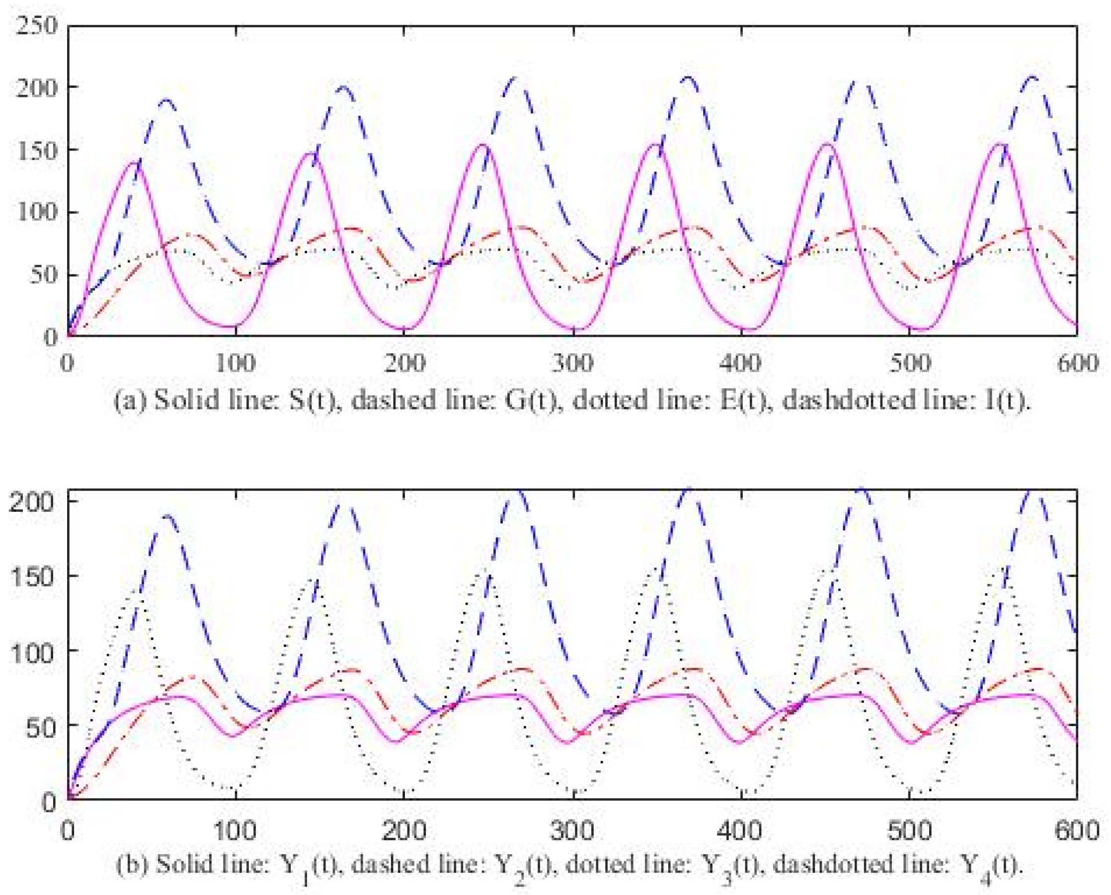
Thus, σ = max{, , , , , , } = 0.8, r = max{||, ||, |, ||} = 0.1042, and σ + r = 0.9042 > 0. The condition of Theorem 2 is satisfied. The system (7) has an oscillatory solution (see Figure 3). In Figure 4, we changed the time delays and kept all parameters the same as in Figure 3. When we selected time delay is so then the unique positive equilibrium point .
Therefore, we can obtain the following:
4. Discussion
Our result provides a criterion to determine whether or not there exists an oscillatory solution for model (6), which includes discrete and distributed delays. The oscillatory solution of the model (6) corresponds to the tremor of Parkinson’s disease. Therefore, our main result is very significant. We also point out that the bifurcation method is hard to deal with in the present model. Because the bifurcation equation about model (10) is as follows:
It can be noted that if , , , are different positive numbers, Equation (24) is a transcendental equation with four variables. Solving Equation (24) and finding the bifurcating points are hard work.
5. Conclusions
In this paper, we discussed the oscillatory behavior of the solutions for a Parkinson’s disease model with discrete and distributed delays. Two theorems were provided to determine the existence of oscillatory solutions, which were easy to inspect to compare the method of bifurcation. We made the change in distributed delay terms as new functions such that the original system became only a discrete system. This method can be used to deal with all distributed systems. We point out that the present criteria are only sufficient conditions.
Funding
This research received no external funding.
Data Availability Statement
All data used are in [3].
Conflicts of Interest
The author declares no conflict of interest.
References
- Tuwairqi, S.M.; Badrah, A.A. Modeling the dynamics of innate and adaptive immune response to Parkinson’s disease with immunotherapy. AIMS Math. 2023, 8, 1800–1832. [Google Scholar] [CrossRef]
- Wang, Z.; Hu, B.; Zhu, L.; Lin, J.; Xu, M.; Wang, D. The possible mechanism of direct feedback projections from basal ganglia to cortex in beta oscillations of Parkinson’s disease: A theoretical evidence in the competing resonance model. Commun. Nonlinear Sci. Numer. Simul. 2023, 120, 107142. [Google Scholar] [CrossRef]
- Wang, Z.; Hu, B.; Zhu, L.; Lin, J.; Xu, M.; Wang, D. Hopf bifurcation analysis for Parkinson oscillation with heterogeneous delays: A theoretical derivation and simulation analysis. Commun. Nonlinear Sci. Numer. Simul. 2022, 114, 106614. [Google Scholar] [CrossRef]
- Kaslik, E.; Kokovics, E.A.; Radulescu, A. Stability and bifurcations in Wilson-Cowan systems with distributed delays, and an application to basal ganglia interactions. Commun. Nonlinear Sci. Numer. Simul. 2022, 104, 105984. [Google Scholar] [CrossRef]
- Wang, Z.; Hu, B.; Zhou, W.; Xu, M.; Wang, D. Hopf bifurcation mechanism analysis in an improved cortex-basal ganlia network with distributed delays: An application to Parkinson’s disease. Chaos Solitons Fractals 2023, 166, 113022. [Google Scholar] [CrossRef]
- Agiza, H.A.; Sohaly, M.A.; Elfouly, M.A. Small two-delay differential equations for Parkinson’s disease models using Taylor series transform. Indian J. Phys. 2023, 97, 39–46. [Google Scholar] [CrossRef]
- Badrah, A.; Tuwairqi, S.A. Modeling the dynamics of innate immune response to Parkinson disease with therapeutic approach. Phys. Biol. 2022, 19, 056004. [Google Scholar] [CrossRef]
- Mukhtar, R.; Chang, C.Y.; Raja, M.A.; Chaudhar, N.I. Design of intelligent neuro-supervised networks for brain electrical activity rhythms of Parkinson’s disease model. Biomimetics 2023, 8, 322. [Google Scholar] [CrossRef]
- Terman, D.; Rubin, J.E.; Yew, A.C.; Wilson, C.J. Activity patterns in a model for the subthalamopallidal network of the basal ganglia. J. Neurosci. 2020, 22, 2963–2976. [Google Scholar] [CrossRef]
- Chen, Y.; Wang, J.; Kang, Y.; Ghori, M.B. Emergence of beta oscillations of a resonance model for Parkinson’s disease. Neural Plast. 2020, 2020, 8824760. [Google Scholar] [CrossRef]
- Geng, X.; Xu, X.; Horn, A.; Li, N.; Ling, Z.; Brown, P.; Wang, S. Intra-operative characterization of subthalamic oscillations in Parkinson’s disease. Clin. Neurophysiol. 2018, 129, 1001–1010. [Google Scholar] [CrossRef] [PubMed]
- Grado, L.L.; Johnson, M.D.; Netoff, T.I. Bayesian adaptive dual control of deep brain stimulation in a computational model of Parkinson’s disease. PLoS Comput. Biol. 2018, 14, 1006606. [Google Scholar] [CrossRef] [PubMed]
- Hu, B.; Xu, M.; Zhu, L.; Wang, Z.; Wang, D. A bidirectional Hopf bifurcation analysis of Parkinson’s oscillation in a simplified basal ganglia model. J. Theor. Biol. 2022, 536, 110979. [Google Scholar] [CrossRef] [PubMed]
- Darcy, N.; Lofredi, R.; Fatly, B.A.; Neumann, W.J.; Hubl, J.; Brucke, C.; Krause, P.; Schneider, G.; Kuhn, A. Spectral and spatial distribution of subthalamic beta peak activity in Parkinson’s disease patients. Exp. Neurol. 2022, 356, 114150. [Google Scholar] [CrossRef] [PubMed]
- Lang, A.E.; Espay, A.J. Disease modification in Parkinson’s disease: Current approaches, challenges, and future considerations. Mov. Disord. 2018, 33, 660–677. [Google Scholar] [CrossRef]
- Raza, C.; Anjum, R. Parkinson’s disease: Mechanisms, translational models and management. Strateg. Life Sci. 2019, 226, 77–90. [Google Scholar] [CrossRef]
- Burke, R.E.; Mally, K. Axon degeneration in Parkinson’s disease. Exp. Neurol. 2013, 246, 71–83. [Google Scholar] [CrossRef]
- Dovonou, A.; Bolduc, C.; Linan, V.S.; Gora, C.; Peralta, M.R.; Levesque, M. Animal models of Parkinson’s disease: Bridging the gap between disease hallmarks and research questions. Trans. Neurodegener. 2023, 12, 36. [Google Scholar] [CrossRef]
- He, B.; Luo, S. Joint modeling of multivariate longitudinal measurements and survival data with applications to Parkinson’s disease. Stat. Methods Med. Res. 2016, 25, 1346–1358. [Google Scholar] [CrossRef]
- Bushnell, D.; Martin, M. Quality of life and Parkinson’s disease: Translation and validation of the US Parkinson’s disease questionnaire (PDQ-39). Qual. Life Res. 1999, 8, 345–350. [Google Scholar] [CrossRef]
- Bakshi, S.; Chelliah, V.; Chen, C.; Graaf, P.H. Mathematical biology models of Parkinson’s disease. CPT Pharmacomet. Syst. Pharmacol. 2019, 8, 77–86. [Google Scholar] [CrossRef] [PubMed]
- Buatois, S.; Retout, S.; Frey, N.; Ueckert, S. Item response theory as an efficient tool to describe a heterogeneous clinical rating scale in de novo idiopathic Parkinson’s disease patients. Pharm. Res. 2017, 34, 2109–2118. [Google Scholar] [CrossRef] [PubMed]
- Kuznetsov, I.A.; Kuznetsov, A.V. What can trigger the onset of Parkinson’s disease—A modeling study based on a compartmental model of alpha-synuclein transport and aggregation in neurons. Math. Biosci. 2016, 278, 22–29. [Google Scholar] [CrossRef] [PubMed]
- Braatz, E.M.; Coleman, R.A. A mathematical model of insulin resistance in Parkinson’s disease. Comput. Biol.Chem. 2015, 56, 84–97. [Google Scholar] [CrossRef] [PubMed]
- Cloutier, M.; Middleton, R.; Wellstead, P. Feedback motif for the pathogenesis of Parkinson’s disease. IET. Syst. Biol. 2012, 6, 86–93. [Google Scholar] [CrossRef] [PubMed]
- Poliquin, P.O.; Chen, J.; Cloutier, M.; Trudeau, L.E.; Jolicoeur, M. Metabolomics and in-silico analysis reveal critical energy deregulations in animal models of Parkinson’s disease. PLoS ONE 2013, 8, e69146. [Google Scholar] [CrossRef] [PubMed]
- Flagmeier, P.; Meisl, G.; Vendruscolo, M.; Galvagnion, C. Mutations associated with familial Parkinson’s disease alter the initiation and amplification step of α-synuclein aggregation. Proc. Natl. Acad. Sci. USA 2016, 113, 10328–10333. [Google Scholar] [CrossRef] [PubMed]
- Lotharius, J.; Brundin, P. Pathogenesis of Parkinson’s disease: Dopamine, vesicles and α-synuclein. Nat. Rev. Neurosci. 2002, 3, 932–942. [Google Scholar] [CrossRef]
- Plotegher, N.; Duchen, M.R. Crosstalk between lysosomes and mitochondria in Parkinson’s disease. Front. Cell Dev. Biol. 2017, 5, 2011–2018. [Google Scholar] [CrossRef]
- Gelders, G.; Baekelandt, V.; Perren, A. Linking neuroinflammation and neurodegeneration in Parkinson’s disease. J. Immunol. Res. 2018, 2018, 4784268. [Google Scholar] [CrossRef]
- Chafee, N. A bifurcation problem for a functional differential equation of finitely retarded type. J. Math. Anal. Appl. 1971, 35, 312–348. [Google Scholar] [CrossRef]
- Feng, C.; Plamondon, R. An oscillatory criterion for a time delayed neural ring network model. Neural Netw. 2012, 29, 70–79. [Google Scholar] [CrossRef] [PubMed]
Figure 1.
Oscillation of the solutions, , and time delay , , , , , , .
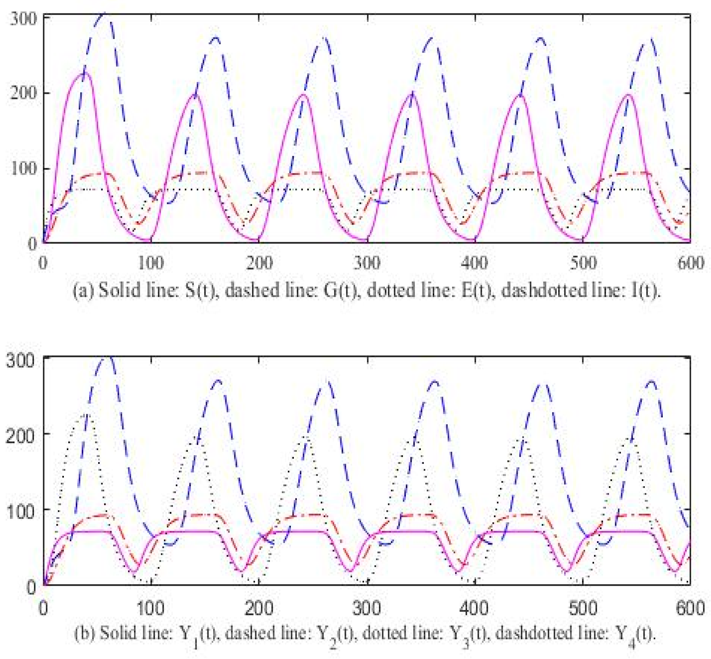
Figure 2.
Oscillation of the solutions, , , , , and time delay , , , , , , , .
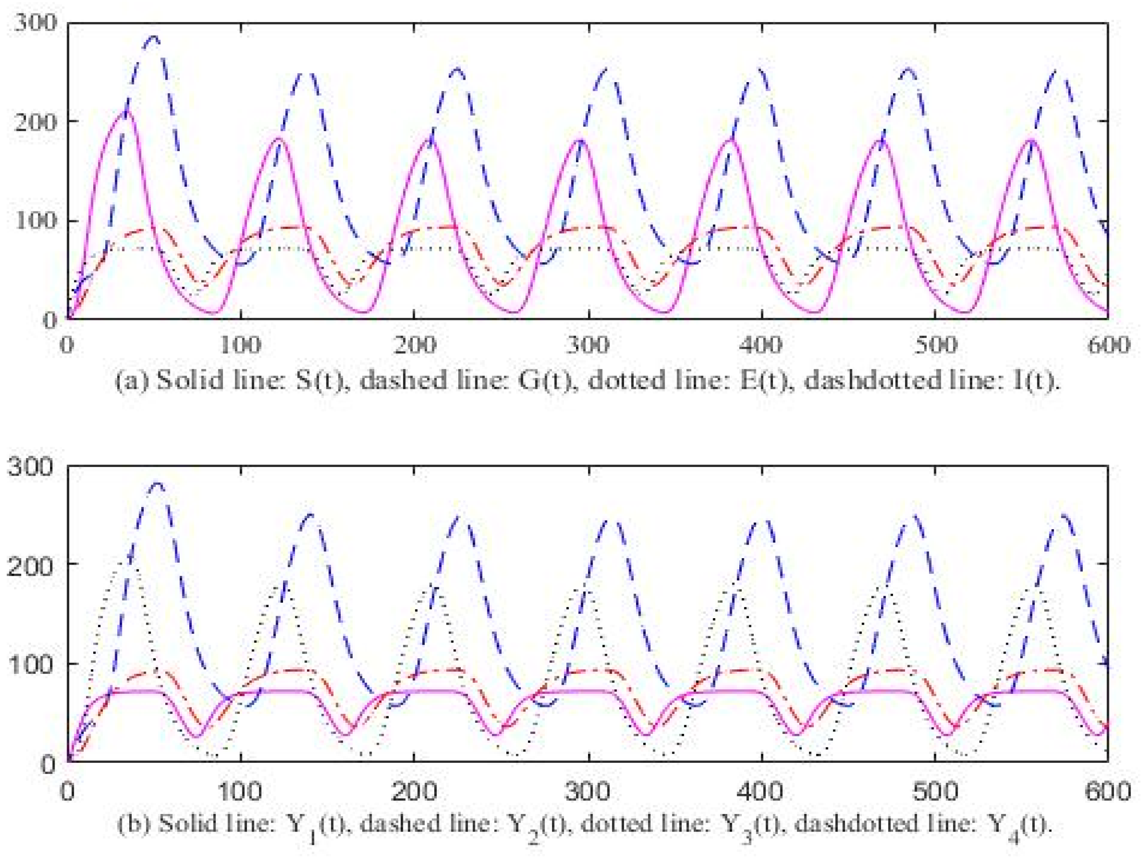
Figure 3.
Oscillation of the solutions, , and time delay , , , , , , , .

Figure 4.
Oscillation of the solutions, , , , , and time delay , , , , , , , .
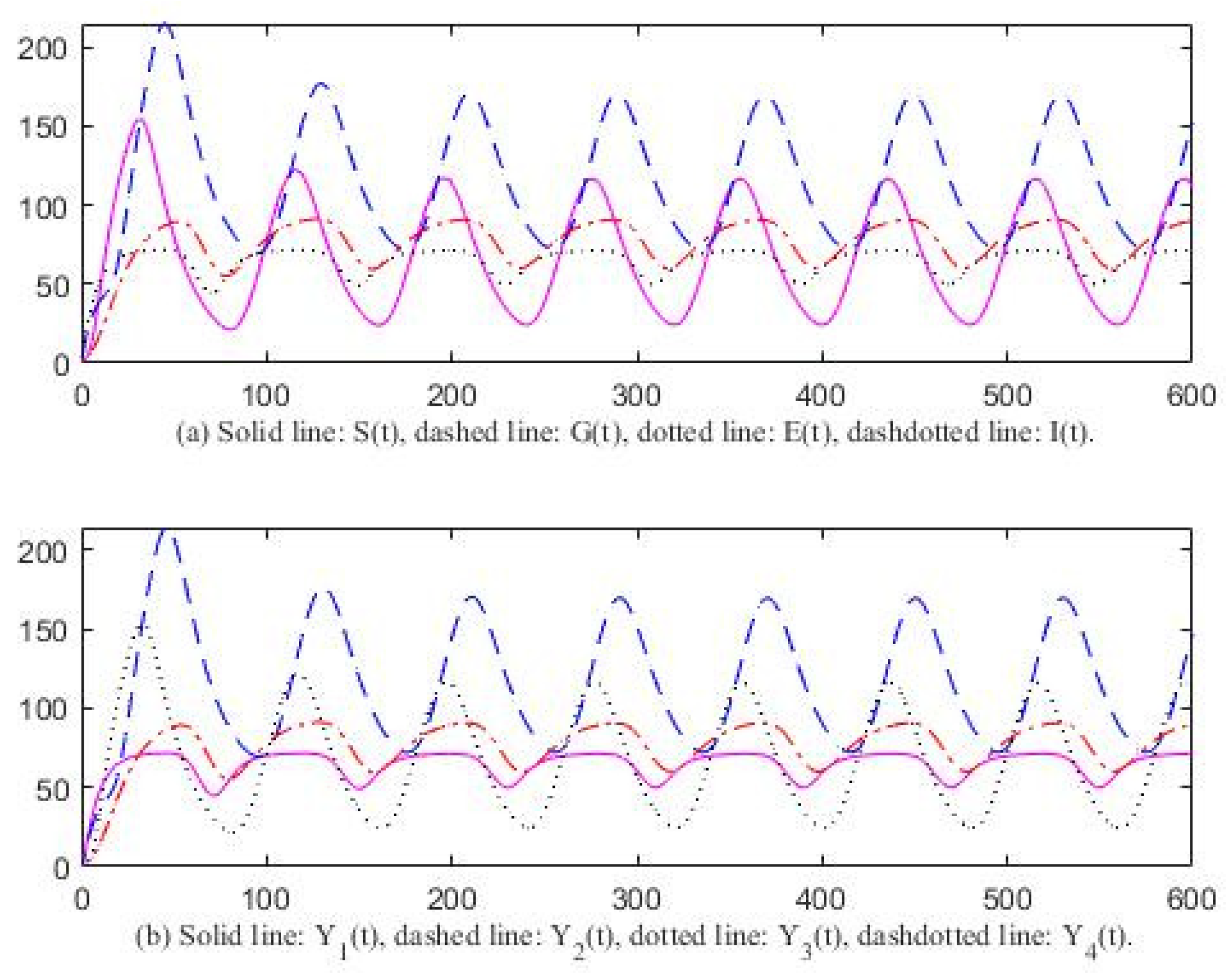
Figure 5.
Oscillation of the solutions, , and time delay , , , , , , , .

Figure 6.
Oscillation of the solutions, , , and time delay , , , , , , , .
Disclaimer/Publisher’s Note: The statements, opinions and data contained in all publications are solely those of the individual author(s) and contributor(s) and not of MDPI and/or the editor(s). MDPI and/or the editor(s) disclaim responsibility for any injury to people or property resulting from any ideas, methods, instructions or products referred to in the content. |
© 2024 by the author. Licensee MDPI, Basel, Switzerland. This article is an open access article distributed under the terms and conditions of the Creative Commons Attribution (CC BY) license (https://creativecommons.org/licenses/by/4.0/).
Share and Cite
MDPI and ACS Style
Feng, C. Oscillatory Behavior of the Solutions for a Parkinson’s Disease Model with Discrete and Distributed Delays. Axioms 2024, 13, 75. https://doi.org/10.3390/axioms13020075
AMA Style
Feng C. Oscillatory Behavior of the Solutions for a Parkinson’s Disease Model with Discrete and Distributed Delays. Axioms. 2024; 13(2):75. https://doi.org/10.3390/axioms13020075
Chicago/Turabian StyleFeng, Chunhua. 2024. "Oscillatory Behavior of the Solutions for a Parkinson’s Disease Model with Discrete and Distributed Delays" Axioms 13, no. 2: 75. https://doi.org/10.3390/axioms13020075
Note that from the first issue of 2016, this journal uses article numbers instead of page numbers. See further details here.