Spherical Linear Diophantine Fuzzy Graphs: Unleashing the Power of Fuzzy Logic for Uncertainty Modeling and Real-World Applications

Abstract

The theory of spherical linear Diophantine fuzzy sets (SLDFS) boasts several advantages over existing fuzzy set (FS) theories such as Picture fuzzy sets (PFS), spherical fuzzy sets (SFS), and T-spherical fuzzy sets (T-SFS). Notably, SLDFS offers a significantly larger portrayal space for acceptable triplets, enabling it to encompass a wider range of ambiguous and uncertain knowledge data sets. This paper delves into the regularity of spherical linear Diophantine fuzzy graphs (SLDFGs), establishing their fundamental concepts. We provide a geometrical interpretation of SLDFGs within a spherical context and define the operations of complement, union, and join, accompanied by illustrative examples. Additionally, we introduce the novel concept of a spherical linear Diophantine isomorphic fuzzy graph and showcase its application through a social network scenario. Furthermore, we explore how this amplified depiction space can be utilized for the study of various graph theoretical topics.

1. Introduction

Many real-world problems have ambiguity and information uncertainties; classical mathematics is not always beneficial. Zadeh [1] created the fuzzy set idea by assigning grades to options ranging from zero to one. This notion is used to represent ambiguity, imprecision, and obscures in a variety of areas [2,3,4]. Zadeh [5] defined the linguistic component for connecting real-world situations to computer simulations. Linguistic index, on the other hand, as per Zadeh [5], is a fluctuating value whose interpretations are phrases or statements in actual or imagined language. The volatile value is known as a fuzzy linguistic variable and such indications are handled by FSs expressed over an innuendo set. Intuitionistic fuzzy sets (IFSs) viewed as an add-on concept of FS since this set include favorable and non-favorable grades, with restriction $0\le \mathfrak{m}+\mathfrak{n}\le 1$, and this theory is founded by Atanassov [6,7,8]. Atanassov [9] offered the geometrical perspective of the IFS. Smarandache [10] conferred the notion of NS of a system as an attached form of FSs and IFSs in 1998. For each choice in the reference set, this framework enables a favorable, an abstinence, and a non-favorable grade. All the grades are distinct from one another and are in the range of [0, 1].

In many complicated real-life situations, knowledge is not always limited to yes or no options, but may also include yes, abstention, no, and denial variants. In 2013, Cuong [11,12,13] revealed the notion of PFS to cope with circumstances like this. This system’s elements represent levels of pleasure, abstinence, and displeasure with constraint $0\le \mathfrak{m}+\mathfrak{a}+\mathfrak{n}\le 1$ and with degree of rejection $\mathfrak{r}=1-(\mathfrak{m}+\mathfrak{a}+\mathfrak{n})$. This technique is comparable to the behavior of human beings and likewise handles decision-making issues. All of the grades are reliant on each other, in consonance with the restriction of the picture fuzzy set, and we are unable to provide the standards of these grades separately from zero to one. Andekah et al. [14] and Mahmood et al. [15,16] introduced a novel concept of a SFS with restriction $0\le {\mathfrak{m}}^{\mathfrak{2}}+{\mathfrak{a}}^{\mathfrak{2}}+{\mathfrak{n}}^{\mathfrak{2}}\le 1$ to overcome the drawbacks stated in PFS. To address the limitations of SFS, they devised a new structure called T-SFS, which satisfies requirement $0\le {\mathfrak{m}}^{\mathfrak{t}}+{\mathfrak{a}}^{\mathfrak{t}}+{\mathfrak{n}}^{\mathfrak{t}}\le 1$, where $\mathfrak{t}=1,2,3,\dots ,n$.

SFSs and T-SFSs have some limits associated with the degrees of favorable, abstinence, and non-favorable grades. Both limitations demonstrate that the grades are interdependent. To overcome these restrictions, a new SLDFS model was proposed by Riaz et al. [17] with constraints $0\le \alpha \mathfrak{m}+\beta \mathfrak{a}+\gamma \mathfrak{n}\le 1$, and the sum of the reference parameters $\alpha ,\beta ,\gamma$ drawn from interval [0, 1] should lie between 0 and 1. These reference values are related to the favorable, abstinence, and non-favorable grades, respectively. The elegance of this new concept is that we can pick any grade in the range of [0, 1] and use reference parameters to classify the framework and manage uncertainty parametrically. We can take all of the grades freely in the NS, but parameterizations are lacking. SLDFS [18,19,20,21] is more effective and more efficient when juxtaposed to the other existing sets such as FS, IFS, PFS, SFS, and T-SFS.

T-Spherical Linear Diophantine Fuzzy Sets (T-SLDFS) [22] are a generalization of the proposed method and address limitations related to reference parameters (RPs). Specifically, the sum of RPs provided by a decision maker is often larger than one ($\mathfrak{m}+\mathfrak{a}+\mathfrak{n}\ge 1$), which violates the restriction of SLDFS. T-SLDFS introduces the qth power of RPs, which covers the space of existing structures and membership grades through the utilization of the qth power of RPs.

Graph theory has been demonstrated to be one of the most potent methods for describing complicated problems because of its simplicity and universality. Graph models have a wide range of applications in economics, operations research, system analysis, and other fields. Clearly, such frameworks must incorporate more structures than just the vertices’ adjacencies. However, because some elements of graph theoretical issues may be unclear in many actual circumstances, it is convenient to deal with all these facets using fuzzy logic approaches.Combining fuzzy logic with machine learning approaches like neural networks or evolutionary algorithms allows for tackling complex, non-linear decision problems effectively [23]. Multi-Granular Fuzzy Logic handles data at different levels of granularity, enabling more flexible and efficient decision-making in complex systems [24].

Kaufmann [25] offered the interpretation of a fuzzy graph (FG). Rosenfeld [26] and Mordeson [27] both described fuzzy graphs. Following that, Bhattacharya [28] expressed his thoughts on “fuzzy graphs”. He demonstrated that none of the principles in crisp graph theory apply to FGs. Thirunavukarasu et al. [29] discovered and investigated the notion of complex fuzzy graphs (CFG). Parvathi and Karunambigai [30] described in detail the intuitionistic fuzzy graph (IFG). The concept of IFGs was studied by many scientists, refs. [10,31,32,33,34,35,36,37,38], which brought valuable results to this field. Zuo et al. [39] in 2019 put forwarded the approach of a picture fuzzy graph (PFG). Akram [40,41] recently studied a spherical fuzzy graph (SFG) and employed the notion in decision-making algorithms. Linear Diophantine fuzzy graphs (LDFG), along with their properties and applications, where studied by many authors recently in [42,43,44]. Guleria and Bajaj [45] defined the notion of a T-spherical fuzzy graph (T-SFG) and applied it for various selection processes.

1.1. Motivation

Traditional fuzzy set (FS) theories like PFS, SFS, T-SFS, and even T-SLDFS struggle to accurately represent complex data sets riddled with ambiguity and uncertainty. Their limited portrayal spaces for membership, non-membership, and neutrality degrees restrict their expressive cost.

This paper leaps forward by introducing spherical linear Diophantine fuzzy sets (SLDFS), which boast a significantly large portrayal space. This enables them to capture a wide range of nuanced and uncertain knowledge data, leading to a faithful representation of real-world scenarios.

Here is what drives the content:

• Filling the void in representational power: We tackle the inherent limitations of existing FS theories and offer SLDFS as a robust solution for situations with intricate vagueness and indeterminacy.
• Many decision-making problems involve complex relationships between entities, often represented as graphs. Traditional fuzzy sets struggle to directly incorporate these relationships into their analysis.
• SLDFSs, when applied to graphs, can explicitly map the degrees of membership, non-membership, and indeterminacy to nodes and edges within the graph. This allows for seamless integration of graph structure into the decision-making process.
• Exploring the uniqueness of SLDFGs: We delve into the structure and behavior of spherical linear Diophantine fuzzy graphs (SLDFGs), establishing their core concepts and providing a clear geometrical interpretation within a spherical framework.
• Formalizing key operations: We define and illustrate the fundamental operations of complement, union, and join for SLDFGs, equipping researchers with essential tools for manipulating and analyzing these structures.
• Introducing isomorphism in SLDFGs: We introduce the novel concept of a spherical linear Diophantine isomorphic fuzzy graph, showcasing its potential through a social network example. This adds a new dimension to the analysis and comparison of SLDFGs.
• Unveiling new research avenues: The expanded portrayal space of SLDFS opens doors for exploring various graph theoretical topics from a fresh perspective. This paper invites further research in this fertile ground.

In essence, the content is driven by a desire to overcome the representational limitations of existing FS theories and introduce a powerful new tool—SLDFS—for grappling with complex and uncertain knowledge domains. The exploration of SLDFGs and their properties paves the way for exciting advancements in graph theory and beyond.

This revised motivation avoids plagiarism by focusing on the unique strengths and applications of SLDFS while emphasizing the research gap it addresses and the new avenues it opens up.

1.2. Objectives

We have the following observations based on the aforementioned discussions:

• SLDFS is sufficiently better than FS, IFS, PFS, NS, SFS and T-SFS to deliberate the fuzzy information/vagueness as it has the reference parameter.
• When dealing with information embedded among multiple alternatives/attributes, the graph-theoretic portrayal of knowledge is more convenient and effective. However, graph representation has never been used with SLDFSs in the literature.
• To cope with decision-making issues, expressions based on the SLDFS concept and its graph-theoretic depictions are expected to be multifariously adaptable and have a wider range of information coverage.
• We introduce the notion of spherical linear Diophantine fuzzy graph with some operations such as join, union and complement. Some properties of SLDFG are also studied.
• To validate the proposed work, a social network problem is considered and the proposed notion is employed in it to obtain the best result.

As a result, the objective of this article is to essentially strengthen graph-theoretic concepts via the spherical linear Diophantine fuzzy environment in order to provide a greater range and depth of knowledge. We initiate SLDFG as a novel type of graph and investigate its properties and usages.

The work in this paper is organized as follows. Section 2 provides some primitive interpretations and preliminaries for the generalized fuzzy sets: IFSs, PFSs, SFSs, T-SFSs, IFG, PFG, SFG, T-SFG. Given the immense capability of SLDFSs with the reference parameter to model the imprecise, incomplete, uncertain, or vague knowledge ingrained in authentic scenarios, a new type of spherical linear Diophantine fuzzy graph is defined in Section 3. Plentiful operations with the introduced graphs are examined in Section 4. In Section 5, application via a spherical linear Diophantine fuzzy network is described to handle social networking issues. In Section 6, a brief comparison study of the proposed notion and its benefits with FS/IFS/PFS/SFS/T-SFS are presented. Finally, in Section 7, the article is closed by outlining the potential for further research.

2. Preliminaries

This section introduces various extensions of fuzzy sets and their corresponding graphs, providing basic definitions for each. We use the below symbols and notation stated in

Table 1. List of acronyms & symbols.

Notations	Abbreviations	Symbols
Intuitionistic fuzzy set	IFS	$\mathfrak{I}$
Spherical linear Diophantine Fuzzy graph	SLDFG	$\mathfrak{G}$
Score function	SF	$S_{\mathfrak{S}}\mathfrak{D}$
Accuracy function	AF	$A_{\mathfrak{S}}\mathfrak{D}$
Spherical linear Diophantine Fuzzy graph order	SLDFGO	$\mathfrak{O}\left(\mathfrak{G}\right)$
Spherical linear Diophantine Fuzzy graph degree	SLDFGD	${\mathfrak{d}}_{\mathfrak{G}}\left(\mathfrak{u}\right)$
Spherical linear Diophantine Fuzzy graph total degree	SLDFGTD	${\mathfrak{d}}_{\mathfrak{G}}\left(\mathfrak{u}\right)$
Strong spherical linear Diophantine fuzzy graph	S-SLDFG	$\mathfrak{SG}$
Spherical linear Diophantine Fuzzy in-degree centrality	SLDFIDC	${\mathfrak{d}}_{\mathfrak{I}}\left({\mathfrak{v}}_{\mathfrak{i}}\right)$
Spherical linear Diophantine Fuzzy out-degree centrality	SLDFODC	${\mathfrak{d}}_{\mathfrak{O}}\left({\mathfrak{v}}_{\mathfrak{i}}\right)$

throughout the paper.

Definition 1 

([6,7,8]). Let $\mathfrak{Q}$ be the universe and let $\mathfrak{I}$ be a set. $\mathfrak{I}$ is said to be an IFS if

$$\mathfrak{I}=\{e,\mathfrak{m}(e),\mathfrak{n}(e\left)\right|e\in \mathfrak{Q}\}$$

where $\mathfrak{m},\mathfrak{n}$ from $\mathfrak{I}$ to $[0,1]$ are the favorable and non-favorable grades, respectively, provided $0\le \mathfrak{m}+\mathfrak{n}\le 1$. The indeterminacy grade is given by $\mathfrak{r}\left(e\right)=1-(\mathfrak{m}+\mathfrak{n}):\forall e\in \mathfrak{Q}$.

Definition 2 

([14,15,16]). SFS $\mathfrak{S}$ on universe $\mathfrak{Q}$ is defined by

$$\mathfrak{S}=\{e,\mathfrak{m}(e),\mathfrak{a}(e),\mathfrak{n}(e\left)\right|e\in \mathfrak{Q}\}$$

where $\mathfrak{m},\mathfrak{a},\mathfrak{n}:\mathfrak{S}\to [0,1]$ are the favorable, abstinence and non-favorable grades, respectively. The constraint for a SFS is that $0\le {\mathfrak{m}}^{\mathfrak{2}}+{\mathfrak{a}}^{\mathfrak{2}}+{\mathfrak{n}}^{\mathfrak{2}}\le 1$. The refusal grade is given by ${\mathfrak{r}}^{\mathfrak{2}}\left(e\right)=1-({\mathfrak{m}}^{\mathfrak{2}}+{\mathfrak{a}}^{\mathfrak{2}}+{\mathfrak{n}}^{\mathfrak{2}}):\forall e\in \mathfrak{Q}$.

Definition 3 

([26]). Let $\mathfrak{Q}\ne \varnothing$ be a reference set. SLDFS ${\mathfrak{S}}_{\mathfrak{D}}$ on $\mathfrak{Q}$ is of the form

$${\mathfrak{S}}_{\mathfrak{D}}=\{(e,\langle {\mathfrak{m}}_{\mathfrak{D}}\left(e\right),{\mathfrak{a}}_{\mathfrak{D}}\left(e\right),{\mathfrak{n}}_{\mathfrak{D}}\left(e\right)\rangle ,\langle {\alpha }_{\mathfrak{D}}\left(e\right),{\beta }_{\mathfrak{D}}\left(e\right),{\eta }_{\mathfrak{D}}\left(e\right)\rangle ):e\in \mathfrak{Q}\}$$

where ${\mathfrak{m}}_{\mathfrak{D}}\left(e\right),{\mathfrak{a}}_{\mathfrak{D}}\left(e\right),{\mathfrak{n}}_{\mathfrak{D}}\left(e\right)$ are favorable grade, abstinence and non-favorable grade, and reference parameters are denoted by $\alpha \left(e\right),\beta \left(e\right),\eta \left(e\right)\in [0,1]$. The triplet pair satisfying constraint $0\le {\alpha }_{\mathfrak{D}}\left(e\right){\mathfrak{m}}_{\mathfrak{D}}\left(e\right)+{\beta }_{\mathfrak{D}}\left(e\right){\mathfrak{a}}_{\mathfrak{D}}\left(e\right)+{\eta }_{\mathfrak{D}}\left(e\right){\mathfrak{n}}_{\mathfrak{D}}\left(e\right)\le 1$ for all $e\in \mathfrak{Q}$ and with $0\le \alpha \left(e\right)+\beta \left(e\right)+\eta \left(e\right)\le 1$.

The refusal grade is defined as ${\gamma }_{\mathfrak{D}}\left(e\right){\mathfrak{r}}_{\mathfrak{D}}=\left(e\right)=1-({\alpha }_{\mathfrak{D}}\left(e\right){\mathfrak{m}}_{\mathfrak{D}}\left(e\right)+{\beta }_{\mathfrak{D}}\left(e\right){\mathfrak{a}}_{\mathfrak{D}}\left(e\right)+{\eta }_{\mathfrak{D}}\left(e\right){\mathfrak{n}}_{\mathfrak{D}}\left(e\right))$, where ${\gamma }_{\mathfrak{D}}\left(e\right)$ is the refusal reference parameter.

Spherical linear Diophantine fuzzy number (SLDFN) is defined as ${\mathfrak{S}}_{\mathfrak{D}}=(\langle {\mathfrak{m}}_{\mathfrak{D}},{\mathfrak{a}}_{\mathfrak{D}},{\mathfrak{n}}_{\mathfrak{D}}\rangle ,\langle {\alpha }_{\mathfrak{D}},$${\beta }_{\mathfrak{D}},{\eta }_{\mathfrak{D}}\rangle )$ with $0\le \alpha +\beta +\eta \le 1$ and $0\le {\alpha }_{\mathfrak{D}}{\mathfrak{m}}_{\mathfrak{D}}+{\beta }_{\mathfrak{D}}{\mathfrak{a}}_{\mathfrak{D}}+{\eta }_{\mathfrak{D}}{\mathfrak{n}}_{\mathfrak{D}}\le 1$.

Definition 4. 

SLDFS on $\mathfrak{Q}$ is called an absolute SLDFS and null or empty SLDFS, respectively,

(i) 

if ${\mathfrak{S}}_{\mathfrak{D}}^{\mathfrak{1}}=\{e,(\langle 1,0,0\rangle ,\langle 1,0,0\rangle ):e\in \mathfrak{Q}\}$.

(ii) 

if ${\mathfrak{S}}_{\mathfrak{D}}^{\mathfrak{0}}=\{e,(\langle 0,0,1\rangle ,\langle 0,0,1\rangle ):e\in \mathfrak{Q}\}$.

Definition 5. 

• The score function (SF) of SLDFN ${\mathfrak{S}}_{\mathfrak{D}}=(\langle {\mathfrak{m}}_{\mathfrak{D}},{\mathfrak{a}}_{\mathfrak{D}},{\mathfrak{n}}_{\mathfrak{D}}\rangle ,\langle {\alpha }_{\mathfrak{D}},{\beta }_{\mathfrak{D}},{\eta }_{\mathfrak{D}}\rangle )$ is displayed and depicted as

  $$S_{\left({\mathfrak{S}}_{\mathfrak{D}}\right)}=\frac{1}{2}[({\mathfrak{m}}_{\mathfrak{D}}-{\mathfrak{a}}_{\mathfrak{D}}-{\mathfrak{n}}_{\mathfrak{D}})+({\alpha }_{\mathfrak{D}}-{\beta }_{\mathfrak{D}}-{\eta }_{\mathfrak{D}})]$$

  where $S:{\mathfrak{S}}_{\mathfrak{D}}\left(\mathfrak{Q}\right)⟶[-1,1]$.
• The accuracy function (AF) of SLDFN ${\mathfrak{S}}_{\mathfrak{D}}=(\langle {\mathfrak{m}}_{\mathfrak{D}},{\mathfrak{a}}_{\mathfrak{D}},{\mathfrak{n}}_{\mathfrak{D}}\rangle ,\langle {\alpha }_{\mathfrak{D}},{\beta }_{\mathfrak{D}},{\eta }_{\mathfrak{D}}\rangle )$ is displayed and depicted as

  $$A_{\left({\mathfrak{S}}_{\mathfrak{D}}\right)}=\frac{1}{2}[\frac{({\mathfrak{m}}_{\mathfrak{D}}+{\mathfrak{a}}_{\mathfrak{D}}+{\mathfrak{n}}_{\mathfrak{D}})}{3}+({\alpha }_{\mathfrak{D}}+{\beta }_{\mathfrak{D}}+{\eta }_{\mathfrak{D}})]$$

  where $A:{\mathfrak{S}}_{\mathfrak{D}}\left(\mathfrak{Q}\right)⟶[0,1]$,
  where ${\mathfrak{S}}_{\mathfrak{D}}\left(\mathfrak{Q}\right)$ is the assembling of all SLDFNs on $\mathfrak{Q}$.

Definition 6. 

Let ${\mathfrak{S}}_{{\mathfrak{D}}_{\mathfrak{1}}}$ and ${\mathfrak{S}}_{{\mathfrak{D}}_{\mathfrak{2}}}$ be SLDFNs, and these SLDFNs can be compared using SF and AF. It is shown below:

(i) 

${\mathfrak{S}}_{{\mathfrak{D}}_{\mathfrak{1}}}>{\mathfrak{S}}_{{\mathfrak{D}}_{\mathfrak{2}}}$ if $S\left({\mathfrak{S}}_{{\mathfrak{D}}_{\mathfrak{1}}}\right)>S\left({\mathfrak{S}}_{{\mathfrak{D}}_{\mathfrak{2}}}\right)$;

(ii) 

${\mathfrak{S}}_{{\mathfrak{D}}_{\mathfrak{1}}}<{\mathfrak{S}}_{{\mathfrak{D}}_{\mathfrak{2}}}$ if $S\left({\mathfrak{S}}_{{\mathfrak{D}}_{\mathfrak{1}}}\right)<S\left({\mathfrak{S}}_{{\mathfrak{D}}_{\mathfrak{2}}}\right)$;

(iii) 

If $S\left({\mathfrak{S}}_{{\mathfrak{D}}_{\mathfrak{1}}}\right)=S\left({\mathfrak{S}}_{{\mathfrak{D}}_{\mathfrak{2}}}\right)$, then

(a) 

${\mathfrak{S}}_{{\mathfrak{D}}_{\mathfrak{1}}}>{\mathfrak{S}}_{{\mathfrak{D}}_{\mathfrak{2}}}$ if $A\left({\mathfrak{S}}_{{\mathfrak{D}}_{\mathfrak{1}}}\right)>A\left({\mathfrak{S}}_{{\mathfrak{D}}_{\mathfrak{2}}}\right)$;

(b) 

${\mathfrak{S}}_{{\mathfrak{D}}_{\mathfrak{1}}}<{\mathfrak{S}}_{{\mathfrak{D}}_{\mathfrak{2}}}$ if $A\left({\mathfrak{S}}_{{\mathfrak{D}}_{\mathfrak{1}}}\right)<A\left({\mathfrak{S}}_{{\mathfrak{D}}_{\mathfrak{2}}}\right)$;

(c) 

${\mathfrak{S}}_{{\mathfrak{D}}_{\mathfrak{1}}}={\mathfrak{S}}_{{\mathfrak{D}}_{\mathfrak{2}}}$ if $A\left({\mathfrak{S}}_{{\mathfrak{D}}_{\mathfrak{1}}}\right)=A\left({\mathfrak{S}}_{{\mathfrak{D}}_{\mathfrak{2}}}\right)$.

Definition 7. 

Let ${\mathfrak{S}}_{{\mathfrak{D}}_{\mathfrak{i}}}=(\langle {\mathfrak{m}}_{{\mathfrak{D}}_{\mathfrak{i}}},{\mathfrak{a}}_{{\mathfrak{D}}_{\mathfrak{i}}},{\mathfrak{n}}_{{\mathfrak{D}}_{\mathfrak{i}}}\rangle ,\langle {\alpha }_{D_i},{\beta }_{D_i},{\eta }_{D_i}\rangle )$ for $\mathfrak{i}\in \mathrm{\Delta }$ be a convene of SLDFNs on $\mathfrak{Q}$ and $\mathfrak{X}>0$; then,

(i) 

${\mathfrak{S}}_{{\mathfrak{D}}_{\mathfrak{1}}}^{\mathfrak{c}}=(\langle {\mathfrak{n}}_{{\mathfrak{D}}_{\mathfrak{1}}},1-{\mathfrak{a}}_{{\mathfrak{D}}_{\mathfrak{1}}},{\mathfrak{m}}_{{\mathfrak{D}}_{\mathfrak{1}}}\rangle ,\langle {\eta }_{D_1},{\beta }_{D_1},{\alpha }_{D_1}\rangle )$;

(ii) 

${\mathfrak{S}}_{{\mathfrak{D}}_{\mathfrak{1}}}={\mathfrak{S}}_{{\mathfrak{D}}_{\mathfrak{2}}}\iff {\mathfrak{m}}_{{\mathfrak{D}}_{\mathfrak{1}}}={\mathfrak{m}}_{{\mathfrak{D}}_{\mathfrak{2}}},{\mathfrak{a}}_{{\mathfrak{D}}_{\mathfrak{1}}}={\mathfrak{a}}_{{\mathfrak{D}}_{\mathfrak{2}}},{\mathfrak{n}}_{{\mathfrak{D}}_{\mathfrak{1}}}={\mathfrak{n}}_{{\mathfrak{D}}_{\mathfrak{2}}},{\alpha }_{D_1}={\alpha }_{D_2},{\beta }_{D_1}={\beta }_{D_2},{\eta }_{D_1}={\eta }_{D_2}$;

(iii) 

${\mathfrak{S}}_{{\mathfrak{D}}_{\mathfrak{1}}}\subseteq {\mathfrak{S}}_{{\mathfrak{D}}_{\mathfrak{2}}}\iff {\mathfrak{m}}_{{\mathfrak{D}}_{\mathfrak{1}}}\le {\mathfrak{m}}_{{\mathfrak{D}}_{\mathfrak{2}}},{\mathfrak{a}}_{{\mathfrak{D}}_{\mathfrak{1}}}\ge {\mathfrak{a}}_{{\mathfrak{D}}_{\mathfrak{2}}},{\mathfrak{n}}_{{\mathfrak{D}}_{\mathfrak{1}}}\ge {\mathfrak{n}}_{{\mathfrak{D}}_{\mathfrak{2}}},{\alpha }_{D_1}\le {\alpha }_{D_2},{\beta }_{D_1}\ge {\beta }_{D_2},{\eta }_{D_1}\ge {\eta }_{D_2}$;

(iv) 

${\mathfrak{S}}_{{\mathfrak{D}}_{\mathfrak{1}}}\oplus {\mathfrak{S}}_{{\mathfrak{D}}_{\mathfrak{2}}}=(\langle {\mathfrak{m}}_{{\mathfrak{D}}_{\mathfrak{1}}}+{\mathfrak{m}}_{{\mathfrak{D}}_{\mathfrak{2}}}-{\mathfrak{m}}_{{\mathfrak{D}}_{\mathfrak{1}}}{\mathfrak{m}}_{{\mathfrak{D}}_{\mathfrak{2}}},{\mathfrak{a}}_{{\mathfrak{D}}_{\mathfrak{1}}}{\mathfrak{a}}_{{\mathfrak{D}}_{\mathfrak{2}}},{\mathfrak{n}}_{{\mathfrak{D}}_{\mathfrak{1}}}{\mathfrak{n}}_{{\mathfrak{D}}_{\mathfrak{2}}}\rangle ,\langle {\alpha }_{D_1}+{\alpha }_{D_2}-{\alpha }_{D_1}{\alpha }_{D_2},$${\beta }_{D_1}{\beta }_{D_2},{\eta }_{D_1}{\eta }_{D_2}\rangle )$;

(v) 

${\mathfrak{S}}_{{\mathfrak{D}}_{\mathfrak{1}}}\otimes {\mathfrak{S}}_{{\mathfrak{D}}_{\mathfrak{2}}}=(\langle {\mathfrak{m}}_{{\mathfrak{D}}_{\mathfrak{1}}}{\mathfrak{m}}_{{\mathfrak{D}}_{\mathfrak{2}}},{\mathfrak{a}}_{{\mathfrak{D}}_{\mathfrak{1}}}+{\mathfrak{a}}_{{\mathfrak{D}}_{\mathfrak{2}}}-{\mathfrak{a}}_{{\mathfrak{D}}_{\mathfrak{1}}}{\mathfrak{a}}_{{\mathfrak{D}}_{\mathfrak{2}}},{\mathfrak{n}}_{{\mathfrak{D}}_{\mathfrak{1}}}+{\mathfrak{n}}_{{\mathfrak{D}}_{\mathfrak{2}}}-{\mathfrak{n}}_{{\mathfrak{D}}_{\mathfrak{1}}}{\mathfrak{n}}_{{\mathfrak{D}}_{\mathfrak{2}}}\rangle ,\langle {\alpha }_{D_1}{\alpha }_{D_2},{\beta }_{D_1}+{\beta }_{D_2}-{\beta }_{D_1}{\beta }_{D_2},{\eta }_{D_1}+{\eta }_{D_2}-{\eta }_{D_1}{\eta }_{D_2}\rangle )$;

(vi) 

${\mathfrak{XS}}_{{\mathfrak{D}}_{\mathfrak{1}}}=(\langle (1-{(1-{\mathfrak{m}}_{{\mathfrak{D}}_{\mathfrak{1}}})}^{\mathfrak{X}}),{\mathfrak{a}}_{{\mathfrak{D}}_{\mathfrak{1}}}^{\mathfrak{X}},{\mathfrak{n}}_{{\mathfrak{D}}_{\mathfrak{1}}}^{\mathfrak{X}}\rangle ,\langle (1-{(1-{\alpha }_{{\mathfrak{D}}_{\mathfrak{1}}})}^{\mathfrak{X}}),{\beta }_{{\mathfrak{D}}_{\mathfrak{1}}}^{\mathfrak{X}},{\eta }_{{\mathfrak{D}}_{\mathfrak{1}}}^{\mathfrak{X}}\rangle )$;

(vii) 

${\mathfrak{S}}_{{\mathfrak{D}}_{\mathfrak{1}}}^{\mathfrak{X}}=(\langle {\mathfrak{m}}_{{\mathfrak{D}}_{\mathfrak{1}}}^{\mathfrak{X}},(1-{(1-{\mathfrak{a}}_{{\mathfrak{D}}_{\mathfrak{1}}})}^{\mathfrak{X}},(1-{(1-{\mathfrak{n}}_{{\mathfrak{D}}_{\mathfrak{1}}})}^{\mathfrak{X}})\rangle ,\langle {\alpha }_{{\mathfrak{D}}_{\mathfrak{1}}}^{\mathfrak{X}},(1-{(1-{\beta }_{{\mathfrak{D}}_{\mathfrak{1}}})}^{\mathfrak{X}},(1-{(1-{\eta }_{{\mathfrak{D}}_{\mathfrak{1}}})}^{\mathfrak{X}})\rangle )$;

(viii) 

${\mathfrak{S}}_{{\mathfrak{D}}_{\mathfrak{1}}}\cup {\mathfrak{S}}_{{\mathfrak{D}}_{\mathfrak{2}}}=(\langle {\mathfrak{m}}_{{\mathfrak{D}}_{\mathfrak{1}}}\vee {\mathfrak{m}}_{{\mathfrak{D}}_{\mathfrak{2}}},{\mathfrak{a}}_{{\mathfrak{D}}_{\mathfrak{1}}}\wedge {\mathfrak{a}}_{{\mathfrak{D}}_{\mathfrak{2}}},{\mathfrak{n}}_{{\mathfrak{D}}_{\mathfrak{1}}}\wedge {\mathfrak{n}}_{{\mathfrak{D}}_{\mathfrak{2}}}\rangle ,\langle {\alpha }_{D_1}\vee {\alpha }_{D_2},{\beta }_{D_1}\wedge {\beta }_{D_2},{\eta }_{D_1}\wedge {\eta }_{D_2}\rangle )$;

(ix) 

${\mathfrak{S}}_{{\mathfrak{D}}_{\mathfrak{1}}}\cap {\mathfrak{S}}_{{\mathfrak{D}}_{\mathfrak{2}}}=(\langle {\mathfrak{m}}_{{\mathfrak{D}}_{\mathfrak{1}}}\wedge {\mathfrak{m}}_{{\mathfrak{D}}_{\mathfrak{2}}},{\mathfrak{a}}_{{\mathfrak{D}}_{\mathfrak{1}}}\vee {\mathfrak{a}}_{{\mathfrak{D}}_{\mathfrak{2}}},{\mathfrak{n}}_{{\mathfrak{D}}_{\mathfrak{1}}}\vee {\mathfrak{n}}_{{\mathfrak{D}}_{\mathfrak{2}}}\rangle ,\langle {\alpha }_{D_1}\wedge {\alpha }_{D_2},{\beta }_{D_1}\vee {\beta }_{D_2},{\eta }_{D_1}\vee {\eta }_{D_2}\rangle )$.

Example 1. 

Let ${\mathfrak{S}}_{{\mathfrak{D}}_{\mathfrak{1}}}=(\langle 0.87,0.47,0.38\rangle ,\langle 0.27,0.32,0.21\rangle )$ and ${\mathfrak{S}}_{{\mathfrak{D}}_{\mathfrak{2}}}=(\langle 0.95,0.27,0.19\rangle ,\langle 0.41,0.31,0.18\rangle )$ be two SLDFNs; then,

(i) 

${\mathfrak{S}}_{{\mathfrak{D}}_{\mathfrak{1}}}^{\mathfrak{c}}=(\langle 0.38,0.53,0.87\rangle ,\langle 0.21,0.68,0.27\rangle )$;

(ii) 

${\mathfrak{S}}_{{\mathfrak{D}}_{\mathfrak{1}}}\subseteq {\mathfrak{S}}_{{\mathfrak{D}}_{\mathfrak{2}}}$ by Definition 7 (iii);

(iii) 

${\mathfrak{S}}_{{\mathfrak{D}}_{\mathfrak{1}}}\oplus {\mathfrak{S}}_{{\mathfrak{D}}_{\mathfrak{2}}}=(\langle 0.99935,0.1269,0.0722\rangle ,\langle 0.5693,0.0992,0.0378\rangle )$;

(iv) 

${\mathfrak{S}}_{{\mathfrak{D}}_{\mathfrak{1}}}\otimes {\mathfrak{S}}_{{\mathfrak{D}}_{\mathfrak{2}}}=(\langle 0.8265,0.6131,0.4978\rangle ,\langle 0.1107,0.5308,0.3522\rangle )$;

(v) 

${\mathfrak{S}}_{{\mathfrak{D}}_{\mathfrak{1}}}\cup {\mathfrak{S}}_{{\mathfrak{D}}_{\mathfrak{2}}}=(\langle 0.95,0.27,0.19\rangle ,\langle 0.41,0.31,0.18\rangle )={\mathfrak{S}}_{{\mathfrak{D}}_{\mathfrak{2}}}$;

(vi) 

${\mathfrak{S}}_{{\mathfrak{D}}_{\mathfrak{1}}}\cap {\mathfrak{S}}_{{\mathfrak{D}}_{\mathfrak{2}}}=(\langle 0.87,0.47,0.38\rangle ,\langle 0.27,0.32,0.21\rangle )={\mathfrak{S}}_{{\mathfrak{D}}_{\mathfrak{1}}}$.

If $\mathfrak{X}=0.2$, subsequently, we have what follows:

(vii) 

${\mathfrak{XS}}_{{\mathfrak{D}}_{\mathfrak{1}}}=(\langle 0.3351,0.8598,0.8241\rangle ,\langle 0.0610,0.7962,0.7319\rangle )$;

(viii) 

${\mathfrak{S}}_{{\mathfrak{D}}_{\mathfrak{1}}}^{\mathfrak{X}}=(\langle 0.9725,0.1192,0.0912\rangle ,\langle 0.7696,0.742,0.461\rangle )$.

3. Spherical Linear Diophantine Fuzzy Graphs

Definition 8. 

Pair $\mathfrak{G}=({\mathfrak{S}}_{\mathfrak{D}};{\mathfrak{S}}_{\mathfrak{P}})$ is called an SLDFG with node set $\mathfrak{V}$, where ${\mathfrak{S}}_{\mathfrak{D}}$ is node set $\mathfrak{V}$ with spherical linear Diophantine fuzzy values and ${\mathfrak{S}}_{\mathfrak{P}}$ is edge set $\mathfrak{E}\subseteq \mathfrak{V}\times \mathfrak{V}$ with spherical linear Diophantine fuzzy values such that

$$\begin{array}{c}{\mathfrak{m}}_{\mathfrak{P}}\left(\mathfrak{u}\mathfrak{v}\right)\le \{{\mathfrak{m}}_{\mathfrak{D}}\left(\mathfrak{u}\right)\wedge {\mathfrak{m}}_{\mathfrak{D}}\left(\mathfrak{v}\right)\},{\alpha }_{\mathfrak{P}}\left(\mathfrak{uv}\right)\le \{{\alpha }_{\mathfrak{D}}\left(\mathfrak{u}\right)\wedge {\alpha }_{\mathfrak{D}}\left(\mathfrak{v}\right)\};\\ {\mathfrak{a}}_{\mathfrak{P}}\left(\mathfrak{u}\mathfrak{v}\right)\le \{{\mathfrak{a}}_{\mathfrak{D}}\left(\mathfrak{u}\right)\vee {\mathfrak{a}}_{\mathfrak{D}}\left(\mathfrak{v}\right)\},{\beta }_{\mathfrak{P}}\left(\mathfrak{uv}\right)\le \{{\beta }_{\mathfrak{D}}\left(\mathfrak{u}\right)\vee {\beta }_{\mathfrak{D}}\left(\mathfrak{v}\right)\\ {\mathfrak{n}}_{\mathfrak{P}}\left(\mathfrak{u}\mathfrak{v}\right)\le \{{\mathfrak{n}}_{\mathfrak{D}}\left(\mathfrak{u}\right)\vee {\mathfrak{n}}_{\mathfrak{D}}\left(\mathfrak{v}\right)\},{\eta }_{\mathfrak{P}}\left(\mathfrak{uv}\right)\le \{{\eta }_{\mathfrak{D}}\left(\mathfrak{u}\right)\vee {\eta }_{\mathfrak{D}}\left(\mathfrak{v}\right)\},\end{array}$$

for all $\mathfrak{u},\mathfrak{v}\in \mathfrak{V}$, where ${\alpha }_{\mathfrak{D}}\left(\mathfrak{u}\right),{\beta }_{\mathfrak{D}}\left(\mathfrak{u}\right),{\eta }_{\mathfrak{D}}\left(\mathfrak{u}\right)$ and ${\alpha }_{\mathfrak{P}}\left(\mathfrak{uv}\right),{\beta }_{\mathfrak{P}}\left(\mathfrak{uv}\right),{\eta }_{\mathfrak{P}}\left(\mathfrak{uv}\right)$ are the reference parameters associated with node $\mathfrak{v}$ and edge $\mathfrak{uv}$, respectively.

Definition 9. 

Let $\mathfrak{G}=({\mathfrak{S}}_{\mathfrak{D}};{\mathfrak{S}}_{\mathfrak{P}})$ be a SLDFG.

• The order of $\mathfrak{G}$ is defined by

  $$\mathfrak{O}\left(\mathfrak{G}\right)=\left(〈\sum _{\mathfrak{u}\in \mathfrak{V}}{\mathfrak{m}}_{\mathfrak{D}}\left(\mathfrak{u}\right),\sum _{\mathfrak{u}\in \mathfrak{V}}{\mathfrak{a}}_{\mathfrak{D}}\left(\mathfrak{u}\right),\sum _{\mathfrak{u}\in \mathfrak{V}}{\mathfrak{n}}_{\mathfrak{D}}\left(\mathfrak{u}\right)〉,〈\sum _{\mathfrak{u}\in \mathfrak{V}}{\alpha }_{\mathfrak{D}}\left(\mathfrak{u}\right),\sum _{\mathfrak{u}\in \mathfrak{V}}{\beta }_{\mathfrak{D}}\left(\mathfrak{u}\right),\sum _{\mathfrak{u}\in \mathfrak{V}}{\eta }_{\mathfrak{D}}\left(\mathfrak{u}\right)〉\right)$$
• The degree of a node $\mathfrak{u}\in \mathfrak{G}$ is defined by

  $${\mathfrak{d}}_{\mathfrak{G}}\left(\mathfrak{u}\right)=\left(〈\sum _{\mathfrak{uv}\in \mathfrak{E}}{\mathfrak{m}}_{\mathfrak{P}}\left(\mathfrak{uv}\right),\sum _{\mathfrak{uv}\in \mathfrak{E}}{\mathfrak{a}}_{\mathfrak{P}}\left(\mathfrak{uv}\right),\sum _{\mathfrak{uv}\in \mathfrak{E}}{\mathfrak{n}}_{\mathfrak{P}}\left(\mathfrak{uv}\right)〉,〈\sum _{\mathfrak{uv}\in \mathfrak{E}}{\alpha }_{\mathfrak{P}}\left(\mathfrak{uv}\right),\sum _{\mathfrak{uv}\in \mathfrak{E}}{\beta }_{\mathfrak{P}}\left(\mathfrak{uv}\right),\sum _{\mathfrak{uv}\in \mathfrak{E}}{\eta }_{\mathfrak{P}}\left(\mathfrak{uv}\right)〉\right)$$
• The total degree of a node $\mathfrak{u}\in \mathfrak{G}$ is defined by

  $${\mathfrak{td}}_{\mathfrak{G}}\left(\mathfrak{u}\right)=(〈\sum _{\mathfrak{uv}\in \mathfrak{E}}{\mathfrak{m}}_{\mathfrak{P}}\left(\mathfrak{uv}\right)+{\mathfrak{m}}_{\mathfrak{D}}\left(\mathfrak{u}\right),\sum _{\mathfrak{uv}\in \mathfrak{E}}{\mathfrak{a}}_{\mathfrak{P}}\left(\mathfrak{uv}\right)+{\mathfrak{a}}_{\mathfrak{D}}\left(\mathfrak{u}\right),\sum _{\mathfrak{uv}\in \mathfrak{E}}{\mathfrak{n}}_{\mathfrak{P}}\left(\mathfrak{uv}\right)+{\mathfrak{n}}_{\mathfrak{D}}\left(\mathfrak{u}\right)〉,$$

  $$〈\sum _{\mathfrak{uv}\in \mathfrak{E}}{\alpha }_{\mathfrak{P}}\left(\mathfrak{uv}\right)+{\alpha }_{\mathfrak{D}}\left(\mathfrak{u}\right),\sum _{\mathfrak{uv}\in \mathfrak{E}}{\beta }_{\mathfrak{P}}\left(\mathfrak{uv}\right)+{\beta }_{\mathfrak{D}}\left(\mathfrak{u}\right),\sum _{\mathfrak{uv}\in \mathfrak{E}}{\eta }_{\mathfrak{P}}\left(\mathfrak{uv}\right)+{\eta }_{\mathfrak{D}}\left(\mathfrak{u}\right)〉)$$

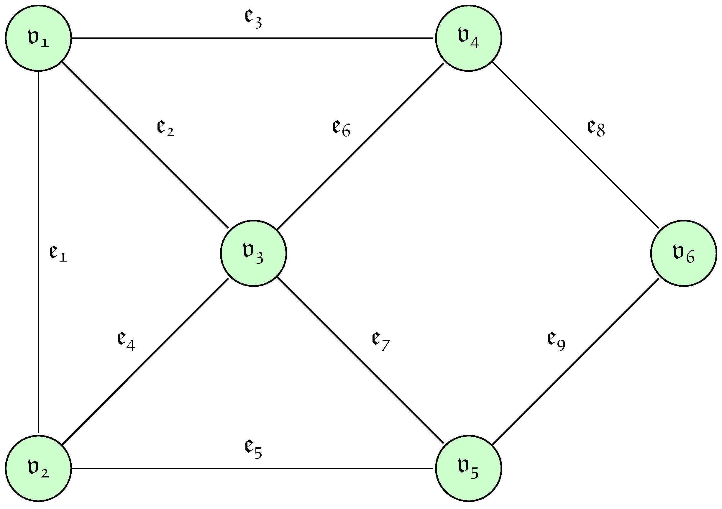
Example 2. 

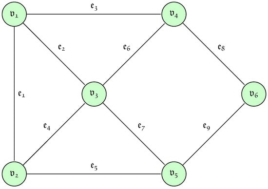
Let $\mathfrak{G}=(\mathfrak{V};\mathfrak{E})$ with vertices $\mathfrak{V}=\{{\mathfrak{v}}_{\mathfrak{1}},{\mathfrak{v}}_{\mathfrak{2}},{\mathfrak{v}}_{\mathfrak{3}},{\mathfrak{v}}_{\mathfrak{4}},{\mathfrak{v}}_{\mathfrak{5}},{\mathfrak{v}}_{\mathfrak{6}}\}$, where the SLDFN of each node is given in

Table 2. The node set with SLDFN of graph $\mathfrak{G}$.

Node	SLDFN = $(\langle {\mathfrak{m}}_{\mathfrak{D}},{\mathfrak{a}}_{\mathfrak{D}},{\mathfrak{n}}_{\mathfrak{D}}\rangle ,\langle {\mathit{\alpha }}_{\mathfrak{D}},{\mathit{\beta }}_{\mathfrak{D}},{\mathit{\eta }}_{\mathfrak{D}}\rangle )$
${\mathfrak{v}}_{\mathfrak{1}}$	$(\langle 0.78,0.63,0.23\rangle ,\langle 0.32,0.21,0.33\rangle )$
${\mathfrak{v}}_{\mathfrak{2}}$	$(\langle 0.61,0.58,0.13\rangle ,\langle 0.35,0.24,0.37\rangle )$
${\mathfrak{v}}_{\mathfrak{3}}$	$(\langle 0.72,0.54,0.33\rangle ,\langle 0.41,0.31,0.12\rangle )$
${\mathfrak{v}}_{\mathfrak{4}}$	$(\langle 0.73,0.51,0.61\rangle ,\langle 0.23,0.32,0.21\rangle )$
${\mathfrak{v}}_{\mathfrak{5}}$	$(\langle 0.67,0.49,0.16\rangle ,\langle 0.15,0.26,0.34\rangle )$
${\mathfrak{v}}_{\mathfrak{6}}$	$(\langle 0.31,0.77,0.27\rangle ,\langle 0.62,0.33,0.19\rangle )$

, the SLDFN of each edge is given in

Table 3. The edge set with SLDFN of graph $\mathfrak{G}$.

Edge	SLDFN = $(\langle {\mathfrak{m}}_{\mathfrak{D}},{\mathfrak{a}}_{\mathfrak{D}},{\mathfrak{n}}_{\mathfrak{D}}\rangle ,\langle {\mathit{\alpha }}_{\mathfrak{D}},{\mathit{\beta }}_{\mathfrak{D}},{\mathit{\eta }}_{\mathfrak{D}}\rangle )$
${\mathfrak{e}}_{\mathfrak{1}}={\mathfrak{v}}_{\mathfrak{1}}{\mathfrak{v}}_{\mathfrak{2}}$	$(\langle 0.60,0.61,0.23\rangle ,\langle 0.30,0.23,0.36\rangle )$
${\mathfrak{e}}_{\mathfrak{2}}={\mathfrak{v}}_{\mathfrak{1}}{\mathfrak{v}}_{\mathfrak{3}}$	$(\langle 0.70,0.62,0.32\rangle ,\langle 0.31,0.29,0.32\rangle )$
${\mathfrak{e}}_{\mathfrak{3}}={\mathfrak{v}}_{\mathfrak{1}}{\mathfrak{v}}_{\mathfrak{4}}$	$(\langle 0.72,0.50,0.61\rangle ,\langle 0.23,0.32,0.33\rangle )$
${\mathfrak{e}}_{\mathfrak{4}}={\mathfrak{v}}_{\mathfrak{2}}{\mathfrak{v}}_{\mathfrak{3}}$	$(\langle 0.60,0.58,0.33\rangle ,\langle 0.34,0.31,0.37\rangle )$
${\mathfrak{e}}_{\mathfrak{5}}={\mathfrak{v}}_{\mathfrak{2}}{\mathfrak{v}}_{\mathfrak{5}}$	$(\langle 0.61,0.57,0.16\rangle ,\langle 0.15,0.26,0.37\rangle )$
${\mathfrak{e}}_{\mathfrak{6}}={\mathfrak{v}}_{\mathfrak{3}}{\mathfrak{v}}_{\mathfrak{4}}$	$(\langle 0.69,0.54,0.33\rangle ,\langle 0.15,0.31,0.34\rangle )$
${\mathfrak{e}}_{\mathfrak{7}}={\mathfrak{v}}_{\mathfrak{3}}{\mathfrak{v}}_{\mathfrak{5}}$	$(\langle 0.65,0.53,0.32\rangle ,\langle 0.14,0.30,0.32\rangle )$
${\mathfrak{e}}_{\mathfrak{8}}={\mathfrak{v}}_{\mathfrak{4}}{\mathfrak{v}}_{\mathfrak{6}}$	$(\langle 0.30,0.73,0.59\rangle ,\langle 0.21,0.33,0.21\rangle )$
${\mathfrak{e}}_{\mathfrak{9}}={\mathfrak{v}}_{\mathfrak{5}}{\mathfrak{v}}_{\mathfrak{6}}$	$(\langle 0.31,0.76,0.25\rangle ,\langle 0.15,0.32,0.31\rangle )$

, the graph is given in Figure 1 and the index matrix is given in

Table 4. Index matrix of SLDFDG $\mathfrak{G}$.

Nodes	${\mathfrak{v}}_{\mathfrak{1}}$	${\mathfrak{v}}_{\mathfrak{2}}$	${\mathfrak{v}}_{\mathfrak{3}}$	${\mathfrak{v}}_{\mathfrak{4}}$	${\mathfrak{v}}_{\mathfrak{5}}$	${\mathfrak{v}}_{\mathfrak{6}}$
${\mathfrak{v}}_{\mathfrak{1}}$	${\mathfrak{L}}_{\mathfrak{D}}^{\mathfrak{0}}$	${\mathfrak{e}}_{\mathfrak{1}}$	${\mathfrak{e}}_{\mathfrak{2}}$	${\mathfrak{e}}_{\mathfrak{3}}$	${\mathfrak{L}}_{\mathfrak{D}}^{\mathfrak{0}}$	${\mathfrak{L}}_{\mathfrak{D}}^{\mathfrak{0}}$
${\mathfrak{v}}_{\mathfrak{2}}$	${\mathfrak{e}}_{\mathfrak{1}}$	${\mathfrak{L}}_{\mathfrak{D}}^{\mathfrak{0}}$	${\mathfrak{e}}_{\mathfrak{4}}$	${\mathfrak{L}}_{\mathfrak{D}}^{\mathfrak{0}}$	${\mathfrak{e}}_{\mathfrak{5}}$	${\mathfrak{L}}_{\mathfrak{D}}^{\mathfrak{0}}$
${\mathfrak{v}}_{\mathfrak{3}}$	${\mathfrak{e}}_{\mathfrak{2}}$	${\mathfrak{e}}_{\mathfrak{4}}$	${\mathfrak{L}}_{\mathfrak{D}}^{\mathfrak{0}}$	${\mathfrak{e}}_{\mathfrak{6}}$	${\mathfrak{e}}_{\mathfrak{7}}$	${\mathfrak{L}}_{\mathfrak{D}}^{\mathfrak{0}}$
${\mathfrak{v}}_{\mathfrak{4}}$	${\mathfrak{e}}_{\mathfrak{3}}$	${\mathfrak{L}}_{\mathfrak{D}}^{\mathfrak{0}}$	${\mathfrak{e}}_{\mathfrak{6}}$	${\mathfrak{L}}_{\mathfrak{D}}^{\mathfrak{0}}$	${\mathfrak{L}}_{\mathfrak{D}}^{\mathfrak{0}}$	${\mathfrak{e}}_{\mathfrak{8}}$
${\mathfrak{v}}_{\mathfrak{5}}$	${\mathfrak{L}}_{\mathfrak{D}}^{\mathfrak{0}}$	${\mathfrak{e}}_{\mathfrak{5}}$	${\mathfrak{e}}_{\mathfrak{7}}$	${\mathfrak{L}}_{\mathfrak{D}}^{\mathfrak{0}}$	${\mathfrak{L}}_{\mathfrak{D}}^{\mathfrak{0}}$	${\mathfrak{e}}_{\mathfrak{9}}$
${\mathfrak{v}}_{\mathfrak{6}}$	${\mathfrak{L}}_{\mathfrak{D}}^{\mathfrak{0}}$	${\mathfrak{L}}_{\mathfrak{D}}^{\mathfrak{0}}$	${\mathfrak{L}}_{\mathfrak{D}}^{\mathfrak{0}}$	${\mathfrak{e}}_{\mathfrak{8}}$	${\mathfrak{e}}_{\mathfrak{9}}$	${\mathfrak{L}}_{\mathfrak{D}}^{\mathfrak{0}}$

.

1.

The order of graph $\mathfrak{O}\left(\mathfrak{G}\right)=(\langle 3.82,3.52,1.73\rangle ,\langle 2.08,1.67,1.56\rangle )$.

2.

The degree of each node is

(i) 

${\mathfrak{d}}_{\mathfrak{G}}\left({\mathfrak{v}}_{\mathfrak{1}}\right)=(\langle 2.02,1.73,1.16\rangle ,\langle 0.84,0.84,1.01\rangle )$;

(ii) 

${\mathfrak{d}}_{\mathfrak{G}}\left({\mathfrak{v}}_{\mathfrak{2}}\right)=(\langle 1.81,1.76,0.72\rangle ,\langle 0.79.0.80,1.10\rangle )$;

(iii) 

${\mathfrak{d}}_{\mathfrak{G}}\left({\mathfrak{v}}_{\mathfrak{3}}\right)=(\langle 2.64,2.27,1.3\rangle ,\langle 0.94,1.21,1.35\rangle )$;

(iv) 

${\mathfrak{d}}_{\mathfrak{G}}\left({\mathfrak{v}}_{\mathfrak{4}}\right)=(\langle 1.71,1.77,1.53\rangle ,\langle 0.59,0.96,0.88\rangle )$;

(v) 

${\mathfrak{d}}_{\mathfrak{G}}\left({\mathfrak{v}}_{\mathfrak{5}}\right)=(\langle 1.57,1.86,0.73\rangle ,\langle 0.44,0.88,1.00\rangle )$;

(vi) 

${\mathfrak{d}}_{\mathfrak{G}}\left({\mathfrak{v}}_{\mathfrak{6}}\right)=(\langle 0.61,1.49,0.84\rangle ,\langle 0.36,0.65,0.52\rangle )$.

3.

The total degree of each node is

(i) 

${\mathfrak{td}}_{\mathfrak{G}}\left({\mathfrak{v}}_{\mathfrak{1}}\right)=(\langle 2.80,2.36,1.39\rangle ,\langle 1.16,1.05,1.34\rangle )$;

(ii) 

${\mathfrak{td}}_{\mathfrak{G}}\left({\mathfrak{v}}_{\mathfrak{2}}\right)=(\langle 2.42,2,34,0,85\rangle ,\langle 1.14,1.04,1.47\rangle )$;

(iii) 

${\mathfrak{td}}_{\mathfrak{G}}\left({\mathfrak{v}}_{\mathfrak{3}}\right)=(\langle 3.36,2.81,1.63\rangle ,\langle 1.35,1.52,1.47\rangle )$;

(iv) 

${\mathfrak{td}}_{\mathfrak{G}}\left({\mathfrak{v}}_{\mathfrak{4}}\right)=(\langle 2.44,2.28,2.14\rangle ,\langle 0.82,1.28,1.09\rangle )$;

(v) 

${\mathfrak{td}}_{\mathfrak{G}}\left({\mathfrak{v}}_{\mathfrak{5}}\right)=(\langle 2.24,2.35,0.89\rangle ,\langle 0.59,1.14,1.34\rangle )$;

(vi) 

${\mathfrak{td}}_{\mathfrak{G}}\left({\mathfrak{v}}_{\mathfrak{6}}\right)=(\langle 0.92,2.26,1.11\rangle ,\langle 0.98,0.98,071\rangle )$.

Definition 10. 

Pair $\mathfrak{SG}=({\mathfrak{S}}_{\mathfrak{D}};{\mathfrak{S}}_{\mathfrak{P}})$ is called a strong spherical linear Diophantine fuzzy graph (S-SLDFG) with node set $\mathfrak{V}$, where ${\mathfrak{S}}_{\mathfrak{D}}$ is the node set with spherical linear Diophantine fuzzy values $\mathfrak{V}$, and ${\mathfrak{S}}_{\mathfrak{P}}$ is the edge set with spherical linear Diophantine fuzzy values $\mathfrak{E}\subseteq \mathfrak{V}\times \mathfrak{V}$ if

$$\begin{array}{c}{\mathfrak{m}}_{\mathfrak{P}}\left(\mathfrak{u}\mathfrak{v}\right)=\{{\mathfrak{m}}_{\mathfrak{D}}\left(\mathfrak{u}\right)\wedge {\mathfrak{m}}_{\mathfrak{D}}\left(\mathfrak{v}\right)\},{\alpha }_{\mathfrak{P}}\left(\mathfrak{uv}\right)=\{{\alpha }_{\mathfrak{D}}\left(\mathfrak{u}\right)\wedge {\alpha }_{\mathfrak{D}}\left(\mathfrak{v}\right)\}\\ {\mathfrak{a}}_{\mathfrak{P}}\left(\mathfrak{u}\mathfrak{v}\right)=\{{\mathfrak{a}}_{\mathfrak{D}}\left(\mathfrak{u}\right)\vee {\mathfrak{a}}_{\mathfrak{D}}\left(\mathfrak{v}\right)\},{\beta }_{\mathfrak{P}}\left(\mathfrak{uv}\right)=\{{\beta }_{\mathfrak{D}}\left(\mathfrak{u}\right)\vee {\beta }_{\mathfrak{D}}\left(\mathfrak{v}\right)\\ {\mathfrak{n}}_{\mathfrak{P}}\left(\mathfrak{u}\mathfrak{v}\right)=\{{\mathfrak{n}}_{\mathfrak{D}}\left(\mathfrak{u}\right)\vee {\mathfrak{n}}_{\mathfrak{D}}\left(\mathfrak{v}\right)\},{\eta }_{\mathfrak{P}}\left(\mathfrak{uv}\right)=\{{\eta }_{\mathfrak{D}}\left(\mathfrak{u}\right)\vee {\eta }_{\mathfrak{D}}\left(\mathfrak{v}\right)\}\end{array}$$

for all $\mathfrak{u},\mathfrak{v}\in \mathfrak{V}$, where ${\alpha }_{\mathfrak{D}}\left(\mathfrak{u}\right),{\beta }_{\mathfrak{D}}\left(\mathfrak{u}\right),{\eta }_{\mathfrak{D}}\left(\mathfrak{u}\right)$ and ${\alpha }_{\mathfrak{P}}\left(\mathfrak{uv}\right),{\beta }_{\mathfrak{P}}\left(\mathfrak{uv}\right),{\eta }_{\mathfrak{P}}\left(\mathfrak{uv}\right)$ are the reference parameters associated with node $\mathfrak{v}$ and edge $\mathfrak{uv}$, respectively.

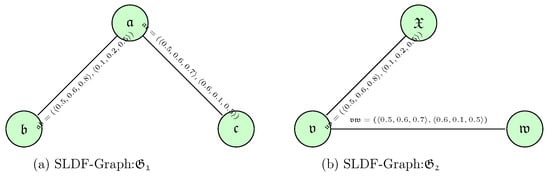
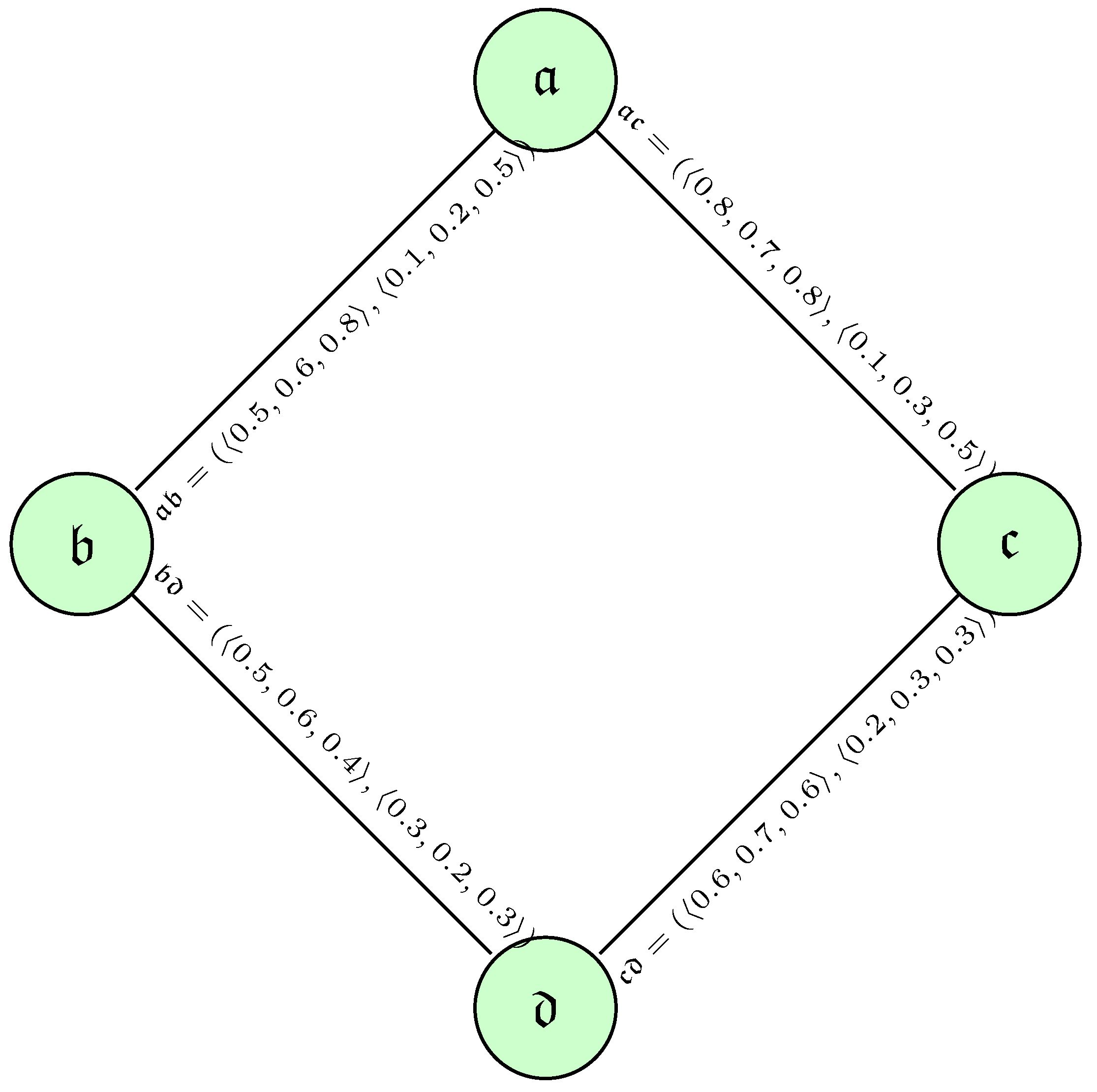
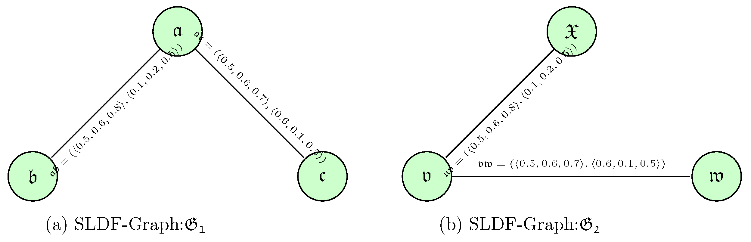
Example 3. 

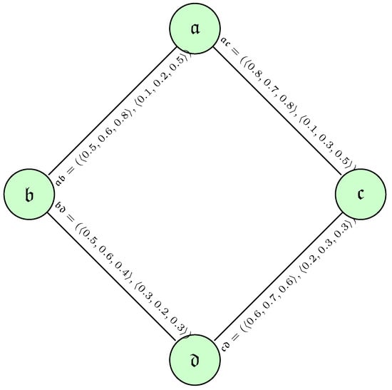
Figure 2 represents a strong spherical linear Diophantine fuzzy graph $\mathfrak{SG}$. The vertices are $\mathfrak{a}=(\langle 0.8,0.6,0.8\rangle ,\langle 0.1,0.2,0.5\rangle )$, $\mathfrak{b}=(\langle 0.5,0.6,0.2\rangle ,\langle 0.3,0.2,0.3\rangle )$, $\mathfrak{c}=(\langle 0.8,0.7,0.6\rangle ,$$\langle 0.2,0.3,0.3\rangle )$, $\mathfrak{d}=(\langle 0.6,0.5,0.4\rangle ,\langle 0.4,0.1,0.3\rangle )$, and the edges are $\mathfrak{ab}=(\langle 0.5,0.6,0.8\rangle ,$$\langle 0.1,0.2,0.5\rangle )$, $\mathfrak{ac}=(\langle 0.8,0.7,0.8\rangle ,\langle 0.1,0.3,0.5\rangle )$, $\mathfrak{bd}=(\langle 0.5,0.6,0.4\rangle ,\langle 0.3,0.2,0.3\rangle )$, $\mathfrak{cd}=(\langle 0.6,0.7,0.6\rangle ,\langle 0.2,0.3,0.3\rangle )$.

4. Spherical Linear Diophantine Fuzzy Graph Operations

In this part, we provide several key graph-theoretic operations on spherical linear Diophantine fuzzy graphs, as well as a number of key findings and instances.

Definition 11. 

The complement of SLDFG $\mathfrak{G}=({\mathfrak{S}}_{\mathfrak{D}};{\mathfrak{S}}_{\mathfrak{P}})$ is SLDFG, and it is represented as $\overline{\mathfrak{G}}=(\overline{{\mathfrak{S}}_{\mathfrak{D}}};\overline{{\mathfrak{S}}_{\mathfrak{P}}})$, defined as

1.

$\overline{{\mathfrak{S}}_{\mathfrak{D}}}={\mathfrak{S}}_{\mathfrak{D}}$;

2.

$\overline{{\mathfrak{m}}_{\mathfrak{D}}}\left(u\right)={\mathfrak{m}}_{\mathfrak{D}}\left(\mathfrak{u}\right)$,$\overline{{\mathfrak{a}}_{\mathfrak{D}}}\left(u\right)={\mathfrak{a}}_{\mathfrak{D}}\left(\mathfrak{u}\right)$,$\overline{{\mathfrak{n}}_{\mathfrak{D}}}\left(u\right)={\mathfrak{n}}_{\mathfrak{D}}\left(\mathfrak{u}\right)$ &

$\overline{{\alpha }_{\mathfrak{D}}}\left(u\right)={\alpha }_{\mathfrak{D}}\left(\mathfrak{u}\right)$,$\overline{{\beta }_{\mathfrak{D}}}\left(u\right)={\beta }_{\mathfrak{D}}\left(\mathfrak{u}\right)$,$\overline{{\eta }_{\mathfrak{D}}}\left(u\right)={\eta }_{\mathfrak{D}}\left(\mathfrak{u}\right)$, for every $\mathfrak{u}\in {\mathfrak{S}}_{\mathfrak{D}}$;

3.

$\overline{{\mathfrak{m}}_{\mathfrak{P}}}\left(uv\right)=\{{\mathfrak{m}}_{\mathfrak{D}}\left(\mathfrak{u}\right)\wedge {\mathfrak{m}}_{\mathfrak{D}}\left(\mathfrak{v}\right)\}-{\mathfrak{m}}_{\mathfrak{P}}\left(uv\right)$, $\overline{{\mathfrak{a}}_{\mathfrak{P}}}\left(uv\right)=\{{\mathfrak{a}}_{\mathfrak{D}}\left(\mathfrak{u}\right)\vee {\mathfrak{a}}_{\mathfrak{D}}\left(\mathfrak{v}\right)\}-{\mathfrak{a}}_{\mathfrak{P}}\left(uv\right)$, $\overline{{\mathfrak{n}}_{\mathfrak{P}}}\left(uv\right)=\{{\mathfrak{n}}_{\mathfrak{D}}\left(\mathfrak{u}\right)\vee {\mathfrak{n}}_{\mathfrak{D}}\left(\mathfrak{v}\right)\}-{\mathfrak{n}}_{\mathfrak{P}}\left(uv\right)$ &

$\overline{{\alpha }_{\mathfrak{P}}}\left(uv\right)=\{{\alpha }_{\mathfrak{D}}\left(\mathfrak{u}\right)\wedge {\alpha }_{\mathfrak{D}}\left(\mathfrak{u}\right)\}-{\alpha }_{\mathfrak{P}}\left(\mathfrak{uv}\right)$, $\overline{{\beta }_{\mathfrak{P}}}\left(uv\right)=\{{\beta }_{\mathfrak{D}}\left(\mathfrak{u}\right)\vee {\beta }_{\mathfrak{D}}\left(\mathfrak{u}\right)\}-{\beta }_{\mathfrak{P}}\left(\mathfrak{uv}\right)$, $\overline{{\beta }_{\mathfrak{P}}}\left(uv\right)=\{{\eta }_{\mathfrak{D}}\left(\mathfrak{u}\right)\vee {\eta }_{\mathfrak{D}}\left(\mathfrak{u}\right)\}-{\eta }_{\mathfrak{P}}\left(\mathfrak{uv}\right)$, for every $\mathfrak{uv}\in {\mathfrak{S}}_{\mathfrak{P}}$.

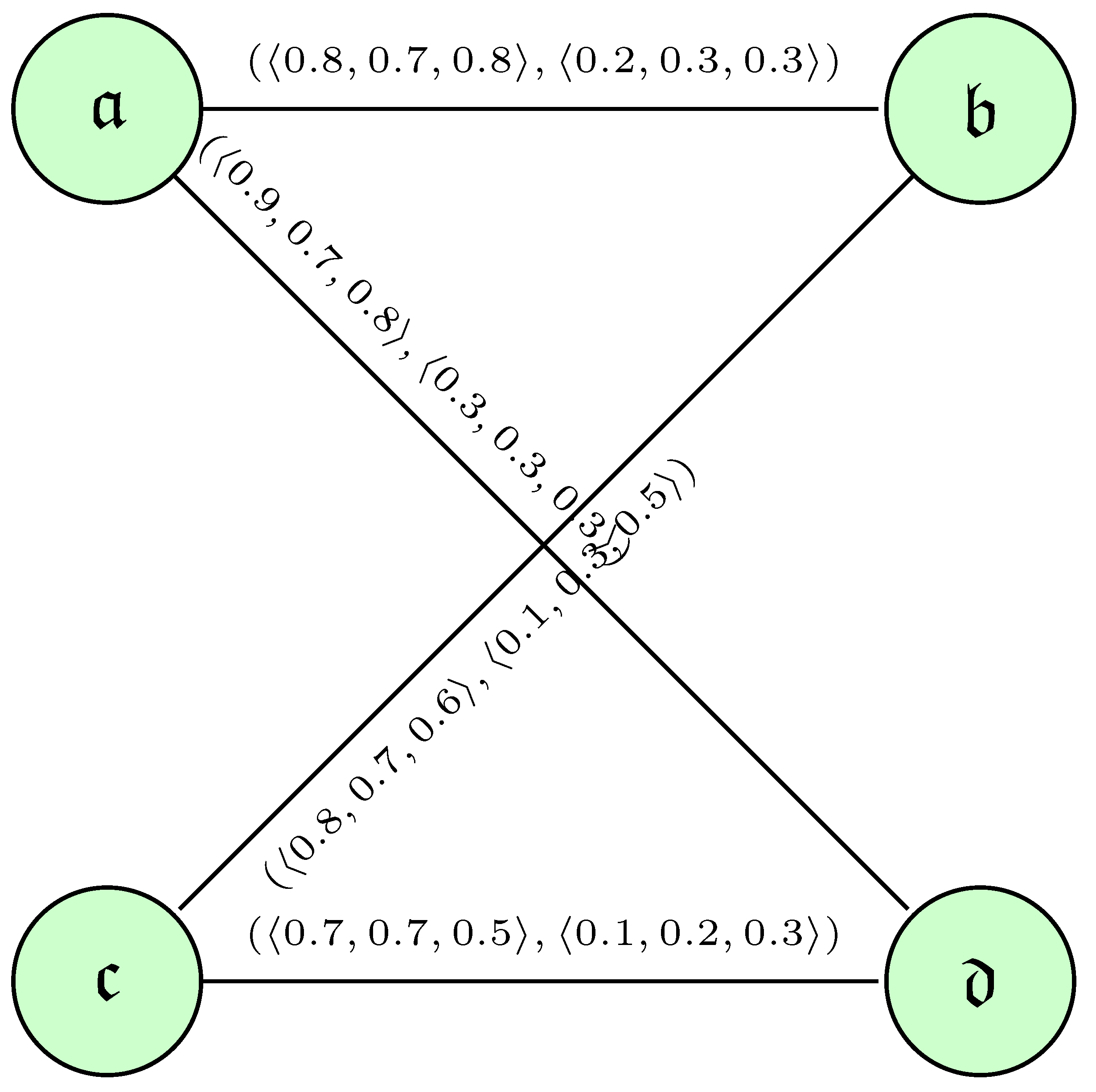
Example 4. 

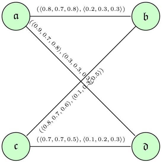
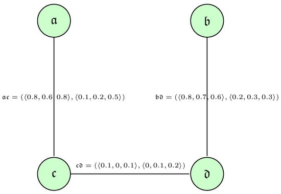
Figure 3 represents spherical linear Diophantine fuzzy graph $\mathfrak{G}$, and its vertices are $\mathfrak{a}=(\langle 0.9,0.4,0.8\rangle ,\langle 0.5,0.2,0.1\rangle )$, $\mathfrak{b}=(\langle 0.8,0.7,0.6\rangle ,\langle 0.2,0.3,0.3\rangle )$, $\mathfrak{c}=(\langle 0.8,0.6,0.4\rangle ,\langle 0.1,0.2,0.5\rangle )$, $\mathfrak{d}=(\langle 0.9,0.7,0.6\rangle ,\langle 0.3,0.3,0.3\rangle )$, and the edges are $\mathfrak{ab}=(\langle 0.8,0.7,0.8\rangle ,\langle 0.2,0.3,0.3\rangle )$, $\mathfrak{ad}=(\langle 0.9,0.7,0.8\rangle ,\langle 0.3,0.3,0.3\rangle )$, $\mathfrak{bc}=(\langle 0.8,0.7,0.6\rangle ,\langle 0.1,0.3,0.5\rangle )$, $\mathfrak{cd}=(\langle 0.7,0.7,0.5\rangle ,\langle 0.1,0.2,0.3\rangle )$.

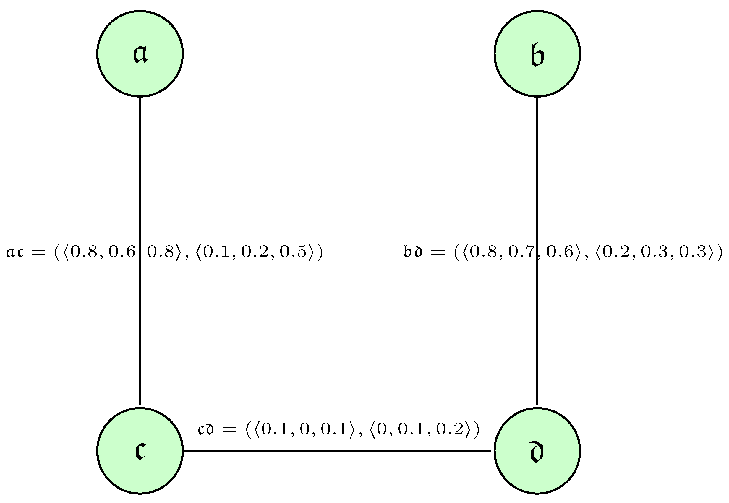
Figure 4 shows the graph of $\overline{\mathfrak{G}}$, which is the complement of $\mathfrak{G}$. The complement edges are $\mathfrak{cd}=(\langle 0.1,0,0.1\rangle ,\langle 0,0.1,0.2\rangle )$, $\mathfrak{ac}=(\langle 0.8,0.6,0.8\rangle ,\langle 0.1,0.2,0.5\rangle )$, $\mathfrak{bd}=(\langle 0.8,0.7,0.6\rangle ,\langle 0.2,0.3,0.3\rangle )$.

Proposition 1. 

If $\mathfrak{SG}$ is a S-SLDFG, then the following holds:

• $\overline{\mathfrak{SG}}$ is also a S-SLDFG;
• $\mathfrak{SG}=\overline{\overline{\mathfrak{SG}}}$.

Definition 12. 

The union of a SLDFG ${\mathfrak{G}}_{\mathfrak{1}}=({\mathfrak{S}}_{{\mathfrak{D}}_{\mathfrak{1}}};{\mathfrak{S}}_{{\mathfrak{P}}_{\mathfrak{1}}})$ and ${\mathfrak{G}}_{\mathfrak{2}}=({\mathfrak{S}}_{{\mathfrak{D}}_{\mathfrak{2}}};{\mathfrak{S}}_{{\mathfrak{P}}_{\mathfrak{2}}})$ is a SLDFG, and it is represented as $\mathfrak{G}={\mathfrak{G}}_{\mathfrak{1}}\cup {\mathfrak{G}}_{\mathfrak{2}}=({\mathfrak{S}}_{{\mathfrak{D}}_{\mathfrak{1}}}\cup {\mathfrak{S}}_{{\mathfrak{D}}_{\mathfrak{2}}};{\mathfrak{S}}_{{\mathfrak{P}}_{\mathfrak{1}}}\cup {\mathfrak{S}}_{{\mathfrak{P}}_{\mathfrak{2}}})$, defined as

$\mathfrak{G}=\left\{\begin{array}{c}\langle {\mathfrak{m}}_{{\mathfrak{D}}_{\mathfrak{1}}}\left(\mathfrak{u}\right),{\mathfrak{a}}_{{\mathfrak{D}}_{\mathfrak{1}}}\left(\mathfrak{u}\right),{\mathfrak{n}}_{{\mathfrak{D}}_{\mathfrak{1}}}\left(\mathfrak{u}\right)\rangle ,\langle {\alpha }_{{\mathfrak{D}}_{\mathfrak{1}}}\left(\mathfrak{u}\right),{\beta }_{{\mathfrak{D}}_{\mathfrak{1}}}\left(\mathfrak{u}\right),{\eta }_{{\mathfrak{D}}_{\mathfrak{1}}}\left(\mathfrak{u}\right)\rangle ,if\mathfrak{u}\in {\mathfrak{V}}_{\mathfrak{1}} and \mathfrak{u}\notin {\mathfrak{V}}_{\mathfrak{2}}\hfill \\ \langle {\mathfrak{m}}_{{\mathfrak{D}}_{\mathfrak{2}}}\left(\mathfrak{u}\right),{\mathfrak{a}}_{{\mathfrak{D}}_{\mathfrak{2}}}\left(\mathfrak{u}\right),{\mathfrak{n}}_{{\mathfrak{D}}_{\mathfrak{2}}}\left(\mathfrak{u}\right)\rangle ,\langle {\alpha }_{{\mathfrak{D}}_{\mathfrak{2}}}\left(\mathfrak{u}\right),{\beta }_{{\mathfrak{D}}_{\mathfrak{2}}}\left(\mathfrak{u}\right),{\eta }_{{\mathfrak{D}}_{\mathfrak{2}}}\left(\mathfrak{u}\right)\rangle ,if\mathfrak{u}\in {\mathfrak{V}}_{\mathfrak{1}} and \mathfrak{u}\notin {\mathfrak{V}}_{\mathfrak{2}},if\mathfrak{u}\notin {\mathfrak{V}}_{\mathfrak{2}} and \mathfrak{u}\in {\mathfrak{V}}_{\mathfrak{1}}\hfill \\ \langle \{{\mathfrak{m}}_{{\mathfrak{D}}_{\mathfrak{1}}}\left(\mathfrak{u}\right)\vee {\mathfrak{m}}_{{\mathfrak{D}}_{\mathfrak{2}}}\left(\mathfrak{u}\right)\},\{{\mathfrak{a}}_{{\mathfrak{D}}_{\mathfrak{1}}}\left(\mathfrak{u}\right)\wedge {\mathfrak{a}}_{{\mathfrak{D}}_{\mathfrak{2}}}\left(\mathfrak{u}\right)\},\{{\mathfrak{n}}_{{\mathfrak{D}}_{\mathfrak{1}}}\left(\mathfrak{u}\right)\wedge {\mathfrak{n}}_{{\mathfrak{D}}_{\mathfrak{2}}}\left(\mathfrak{u}\right)\}\rangle ,\hfill \\ \langle \{{\alpha }_{{\mathfrak{D}}_{\mathfrak{1}}}\left(\mathfrak{u}\right)\vee {\alpha }_{{\mathfrak{D}}_{\mathfrak{2}}}\left(\mathfrak{u}\right)\},\{{\beta }_{{\mathfrak{D}}_{\mathfrak{1}}}\left(\mathfrak{u}\right)\wedge {\beta }_{{\mathfrak{D}}_{\mathfrak{2}}}\left(\mathfrak{u}\right)\},\{{\eta }_{{\mathfrak{D}}_{\mathfrak{1}}}\left(\mathfrak{u}\right)\wedge {\eta }_{{\mathfrak{D}}_{\mathfrak{2}}}\left(\mathfrak{u}\right)\}\rangle if\mathfrak{u}\in {\mathfrak{V}}_{\mathfrak{2}}\cup {\mathfrak{V}}_{\mathfrak{1}}\hfill \end{array}\right.$

$\mathfrak{G}=\left\{\begin{array}{c}\langle {\mathfrak{m}}_{{\mathfrak{D}}_{\mathfrak{1}}}\left(\mathfrak{u}\right),{\mathfrak{a}}_{{\mathfrak{D}}_{\mathfrak{1}}}\left(\mathfrak{u}\right),{\mathfrak{n}}_{{\mathfrak{D}}_{\mathfrak{1}}}\left(\mathfrak{u}\right)\rangle ,\langle {\alpha }_{{\mathfrak{D}}_{\mathfrak{1}}}\left(\mathfrak{u}\right),{\beta }_{{\mathfrak{D}}_{\mathfrak{1}}}\left(\mathfrak{u}\right),{\eta }_{{\mathfrak{D}}_{\mathfrak{1}}}\left(\mathfrak{u}\right)\rangle ,if\mathfrak{u}\in {\mathfrak{V}}_{\mathfrak{1}} and \mathfrak{u}\notin {\mathfrak{V}}_{\mathfrak{2}}\hfill \\ \langle {\mathfrak{m}}_{{\mathfrak{D}}_{\mathfrak{2}}}\left(\mathfrak{uv}\right),{\mathfrak{a}}_{{\mathfrak{D}}_{\mathfrak{2}}}\left(\mathfrak{uv}\right),{\mathfrak{n}}_{{\mathfrak{D}}_{\mathfrak{2}}}\left(\mathfrak{u}\right)\rangle ,\langle {\alpha }_{{\mathfrak{D}}_{\mathfrak{2}}}\left(\mathfrak{uv}\right),{\beta }_{{\mathfrak{D}}_{\mathfrak{2}}}\left(\mathfrak{uv}\right),{\eta }_{{\mathfrak{D}}_{\mathfrak{2}}}\left(\mathfrak{uv}\right)\rangle ,if\mathfrak{uv}\in {\mathfrak{V}}_{\mathfrak{1}} and \mathfrak{uv}\notin {\mathfrak{V}}_{\mathfrak{2}},if\mathfrak{uv}\notin {\mathfrak{V}}_{\mathfrak{2}} and \mathfrak{uv}\in {\mathfrak{V}}_{\mathfrak{1}}\hfill \\ \langle \{{\mathfrak{m}}_{{\mathfrak{D}}_{\mathfrak{1}}}\left(\mathfrak{uv}\right)\vee {\mathfrak{m}}_{{\mathfrak{D}}_{\mathfrak{2}}}\left(\mathfrak{uv}\right)\},\{{\mathfrak{a}}_{{\mathfrak{D}}_{\mathfrak{1}}}\left(\mathfrak{uv}\right)\wedge {\mathfrak{a}}_{{\mathfrak{D}}_{\mathfrak{2}}}\left(\mathfrak{uv}\right)\},\{{\mathfrak{n}}_{{\mathfrak{D}}_{\mathfrak{1}}}\left(\mathfrak{uv}\right)\wedge {\mathfrak{n}}_{{\mathfrak{D}}_{\mathfrak{2}}}\left(\mathfrak{uv}\right)\}\rangle ,\hfill \\ \langle \{{\alpha }_{{\mathfrak{D}}_{\mathfrak{1}}}\left(\mathfrak{uv}\right)\vee {\alpha }_{{\mathfrak{D}}_{\mathfrak{2}}}\left(\mathfrak{uv}\right)\},\{{\beta }_{{\mathfrak{D}}_{\mathfrak{1}}}\left(\mathfrak{uv}\right)\wedge {\beta }_{{\mathfrak{D}}_{\mathfrak{2}}}\left(\mathfrak{uv}\right)\},\{{\eta }_{{\mathfrak{D}}_{\mathfrak{1}}}\left(\mathfrak{uv}\right)\wedge {\eta }_{{\mathfrak{D}}_{\mathfrak{2}}}\left(\mathfrak{uv}\right)\}\rangle if\mathfrak{uv}\in {\mathfrak{V}}_{\mathfrak{2}}\cup {\mathfrak{V}}_{\mathfrak{1}}\hfill \end{array}\right.$

Definition 13. 

The join of a SLDFG ${\mathfrak{G}}_{\mathfrak{1}}=({\mathfrak{S}}_{{\mathfrak{D}}_{\mathfrak{1}}};{\mathfrak{S}}_{{\mathfrak{P}}_{\mathfrak{1}}})$ and ${\mathfrak{G}}_{\mathfrak{2}}=({\mathfrak{S}}_{{\mathfrak{D}}_{\mathfrak{2}}};{\mathfrak{S}}_{{\mathfrak{P}}_{\mathfrak{2}}})$ is a SLDFG and it is represented as $\mathfrak{G}={\mathfrak{G}}_{\mathfrak{1}}+{\mathfrak{G}}_{\mathfrak{2}}=({\mathfrak{S}}_{{\mathfrak{D}}_{\mathfrak{1}}}+{\mathfrak{S}}_{{\mathfrak{D}}_{\mathfrak{2}}};{\mathfrak{S}}_{{\mathfrak{P}}_{\mathfrak{1}}}+{\mathfrak{S}}_{{\mathfrak{P}}_{\mathfrak{2}}})$, defined as

$\mathfrak{G}=\left\{\begin{array}{c}\langle {\mathfrak{m}}_{{\mathfrak{D}}_{\mathfrak{1}}}\left(\mathfrak{u}\right),{\mathfrak{a}}_{{\mathfrak{D}}_{\mathfrak{1}}}\left(\mathfrak{u}\right),{\mathfrak{n}}_{{\mathfrak{D}}_{\mathfrak{1}}}\left(\mathfrak{u}\right)\rangle ,\langle {\alpha }_{{\mathfrak{D}}_{\mathfrak{1}}}\left(\mathfrak{u}\right),{\beta }_{{\mathfrak{D}}_{\mathfrak{1}}}\left(\mathfrak{u}\right),{\eta }_{{\mathfrak{D}}_{\mathfrak{1}}}\left(\mathfrak{u}\right)\rangle ,if\mathfrak{u}\in {\mathfrak{V}}_{\mathfrak{1}} and \mathfrak{u}\notin {\mathfrak{V}}_{\mathfrak{2}}\hfill \\ \langle {\mathfrak{m}}_{{\mathfrak{D}}_{\mathfrak{2}}}\left(\mathfrak{u}\right),{\mathfrak{a}}_{{\mathfrak{D}}_{\mathfrak{2}}}\left(\mathfrak{u}\right),{\mathfrak{n}}_{{\mathfrak{D}}_{\mathfrak{2}}}\left(\mathfrak{u}\right)\rangle ,\langle {\alpha }_{{\mathfrak{D}}_{\mathfrak{2}}}\left(\mathfrak{u}\right),{\beta }_{{\mathfrak{D}}_{\mathfrak{2}}}\left(\mathfrak{u}\right),{\eta }_{{\mathfrak{D}}_{\mathfrak{2}}}\left(\mathfrak{u}\right)\rangle ,if\mathfrak{u}\in {\mathfrak{V}}_{\mathfrak{1}} and \mathfrak{u}\notin {\mathfrak{V}}_{\mathfrak{2}},if\mathfrak{u}\notin {\mathfrak{V}}_{\mathfrak{2}} and \mathfrak{u}\in {\mathfrak{V}}_{\mathfrak{1}}\hfill \\ \langle \left\{{\mathfrak{m}}_{{\mathfrak{D}}_{\mathfrak{1}}\cup {\mathfrak{D}}_{\mathfrak{2}}}\left(\mathfrak{u}\right)\right\},\left\{{\mathfrak{a}}_{{\mathfrak{D}}_{\mathfrak{1}}\cup {\mathfrak{D}}_{\mathfrak{2}}}\left(\mathfrak{u}\right)\right\},\left\{{\mathfrak{n}}_{{\mathfrak{D}}_{\mathfrak{1}}\cup {\mathfrak{D}}_{\mathfrak{2}}}\left(\mathfrak{u}\right)\right\}\rangle ,\hfill \\ \langle \left\{{\alpha }_{{\mathfrak{D}}_{\mathfrak{1}}\cup {\mathfrak{D}}_{\mathfrak{2}}}\left(\mathfrak{u}\right)\right\},\left\{{\beta }_{{\mathfrak{D}}_{\mathfrak{1}}\cup {\mathfrak{D}}_{\mathfrak{2}}}\left(\mathfrak{u}\right)\right\},\left\{{\eta }_{{\mathfrak{D}}_{\mathfrak{1}}\cup {\mathfrak{D}}_{\mathfrak{2}}}\left(\mathfrak{u}\right)\right\}\rangle if\mathfrak{u}\in {\mathfrak{V}}_{\mathfrak{2}}\cup {\mathfrak{V}}_{\mathfrak{1}}\hfill \end{array}\right.$

$\mathfrak{G}=\left\{\begin{array}{c}\langle {\mathfrak{m}}_{{\mathfrak{D}}_{\mathfrak{1}}}\left(\mathfrak{uv}\right),{\mathfrak{a}}_{{\mathfrak{D}}_{\mathfrak{1}}}\left(\mathfrak{uv}\right),{\mathfrak{n}}_{{\mathfrak{D}}_{\mathfrak{1}}}\left(\mathfrak{uv}\right)\rangle ,\langle {\alpha }_{{\mathfrak{D}}_{\mathfrak{1}}}\left(\mathfrak{uv}\right),{\beta }_{{\mathfrak{D}}_{\mathfrak{1}}}\left(\mathfrak{uv}\right),{\eta }_{{\mathfrak{D}}_{\mathfrak{1}}}\left(\mathfrak{uv}\right)\rangle ,if\mathfrak{uv}\in {\mathfrak{V}}_{\mathfrak{1}} and \mathfrak{uv}\notin {\mathfrak{V}}_{\mathfrak{2}}\hfill \\ \langle {\mathfrak{m}}_{{\mathfrak{D}}_{\mathfrak{2}}}\left(\mathfrak{uv}\right),{\mathfrak{a}}_{{\mathfrak{D}}_{\mathfrak{2}}}\left(\mathfrak{uv}\right),{\mathfrak{n}}_{{\mathfrak{D}}_{\mathfrak{2}}}\left(\mathfrak{uv}\right)\rangle ,\langle {\alpha }_{{\mathfrak{D}}_{\mathfrak{2}}}\left(\mathfrak{uv}\right),{\beta }_{{\mathfrak{D}}_{\mathfrak{2}}}\left(\mathfrak{uv}\right),{\eta }_{{\mathfrak{D}}_{\mathfrak{2}}}\left(\mathfrak{uv}\right)\rangle ,if\mathfrak{uv}\in {\mathfrak{V}}_{\mathfrak{1}} and \mathfrak{uv}\notin {\mathfrak{V}}_{\mathfrak{2}} \left(or\right)if\mathfrak{uv}\notin {\mathfrak{V}}_{\mathfrak{2}} and \mathfrak{uv}\in {\mathfrak{V}}_{\mathfrak{1}}\hfill \\ \langle \left\{{\mathfrak{m}}_{{\mathfrak{D}}_{\mathfrak{1}}\cup {\mathfrak{D}}_{\mathfrak{2}}}\left(\mathfrak{uv}\right)\right\},\left\{{\mathfrak{a}}_{{\mathfrak{D}}_{\mathfrak{1}}\cup {\mathfrak{D}}_{\mathfrak{2}}}\left(\mathfrak{uv}\right)\right\},\left\{{\mathfrak{n}}_{{\mathfrak{D}}_{\mathfrak{1}}\cup {\mathfrak{D}}_{\mathfrak{2}}}\left(\mathfrak{uv}\right)\right\}\rangle ,\hfill \\ \langle \left\{{\alpha }_{{\mathfrak{D}}_{\mathfrak{1}}\cup {\mathfrak{D}}_{\mathfrak{2}}}\left(\mathfrak{uv}\right)\right\},\left\{{\beta }_{{\mathfrak{D}}_{\mathfrak{1}}\cup {\mathfrak{D}}_{\mathfrak{2}}}\left(\mathfrak{uv}\right)\right\},\left\{{\eta }_{{\mathfrak{D}}_{\mathfrak{1}}\cup {\mathfrak{D}}_{\mathfrak{2}}}\left(\mathfrak{uv}\right)\right\}\rangle if\mathfrak{uv}\in {\mathfrak{V}}_{\mathfrak{2}}\cup {\mathfrak{V}}_{\mathfrak{1}}\hfill \end{array}\right.$

The following example is used to support the embellishment of the SLDF-union and the SLD-join operation:

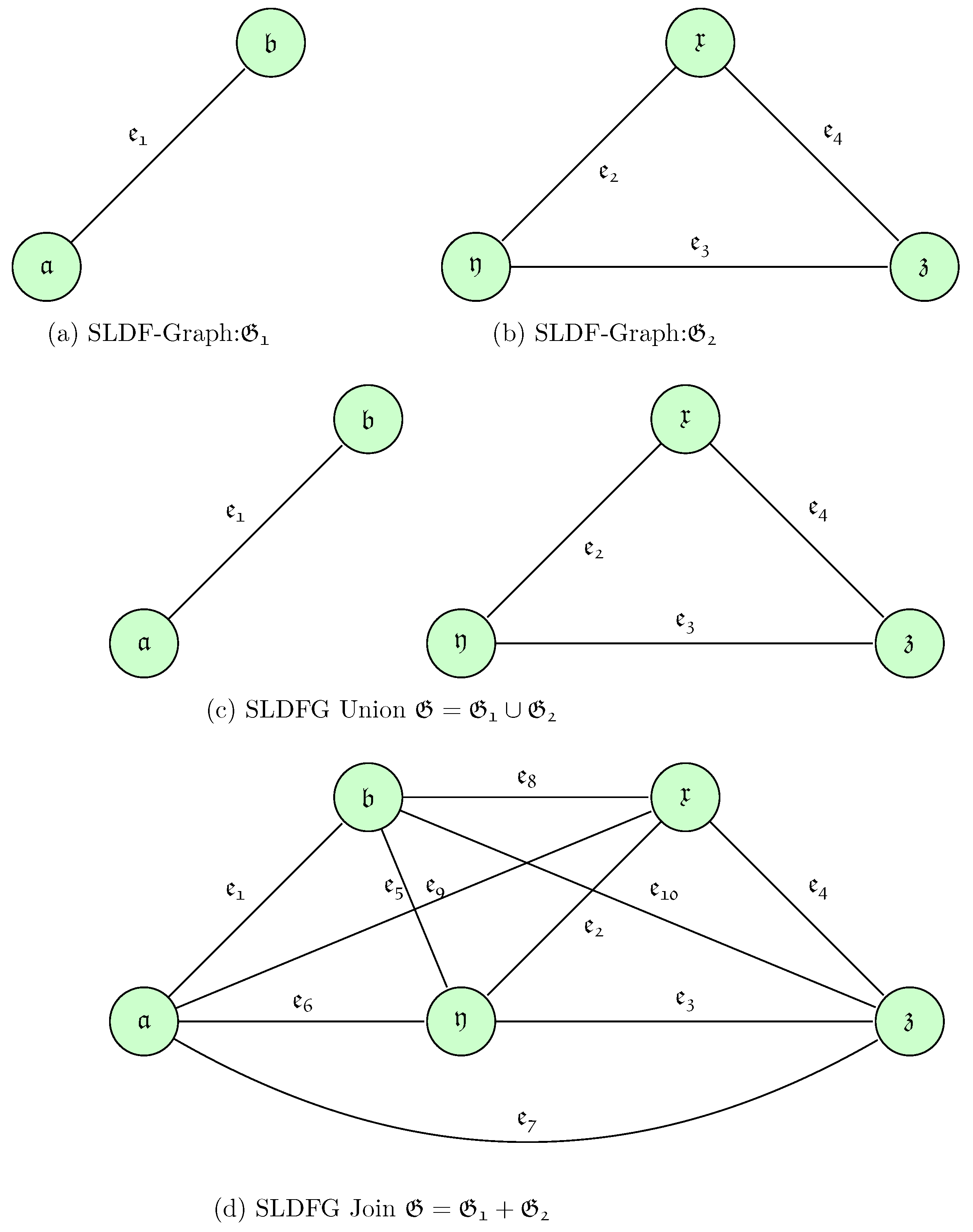
Example 5. 

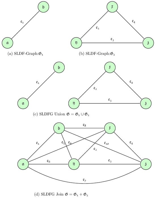
Figure 5 explains the union and join of two SLDFGs. Figure 5a,b represents two spherical linear Diophantine fuzzv graphs ${\mathfrak{G}}_{\mathfrak{1}}$, ${\mathfrak{G}}_{\mathfrak{2}}$.

The vertices of ${\mathfrak{G}}_{\mathfrak{1}}$ are $\mathfrak{a}=(\langle 0.5,0.6,0.7\rangle ,\langle 0.5,0.3,0.1\rangle )$, $\mathfrak{b}=(\langle 0.8,0.3,0.4\rangle ,\langle 0.6,0.2,0.1\rangle )$.

The vertices of ${\mathfrak{G}}_{\mathfrak{2}}$ are $\mathfrak{x}=(\langle 0.9,0.2,0.1\rangle ,\langle 0.4,0.4,0.1\rangle )$, $\mathfrak{y}=(\langle 0.6,0.7,0.5\rangle ,\langle 0.3,0.2,0.4\rangle )$, and $\mathfrak{z}=(\langle 0.7,0.3,0.4\rangle ,\langle 0.5,0.2,0.2\rangle )$. The edges of ${\mathfrak{G}}_{\mathfrak{1}}$ are $\mathfrak{ab}=(\langle 0.5,0.6,0.7\rangle ,\langle 0.5,0.3,0.1\rangle )$. The edges of ${\mathfrak{G}}_{\mathfrak{2}}$ are $\mathfrak{xy}=(\langle 0.6,0.7,0.5\rangle ,\langle 0.3,0.4,0.4\rangle )$, $\mathfrak{yz}=(\langle 0.6,0.7,0.5\rangle ,\langle 0.3,0.2,0.4\rangle )$, $\mathfrak{xz}=(\langle 0.7,0.3,0.4\rangle ,\langle 0.4,0.4,0.2\rangle )$.

$\mathfrak{G}={\mathfrak{G}}_{\mathfrak{1}}\cup {\mathfrak{G}}_{\mathfrak{2}}$ is shown in Figure 5c, and $\mathfrak{G}={\mathfrak{G}}_{\mathfrak{1}}+{\mathfrak{G}}_{\mathfrak{2}}$ is shown in Figure 5d, which are the results of union and join of ${\mathfrak{G}}_{\mathfrak{1}}$, ${\mathfrak{G}}_{\mathfrak{2}}$ respectively. The edge set of the union and the join of ${\mathfrak{G}}_{\mathfrak{1}}$, ${\mathfrak{G}}_{\mathfrak{2}}$ are given in

Table 5. The edge set with SLDFN of graph ${\mathfrak{G}}_{\mathfrak{1}}\cup {\mathfrak{G}}_{\mathfrak{2}}$.

Edge	SLDFN = $(\langle {\mathfrak{m}}_{\mathfrak{D}},{\mathfrak{a}}_{\mathfrak{D}},{\mathfrak{n}}_{\mathfrak{D}}\rangle ,\langle {\mathit{\alpha }}_{\mathfrak{D}},{\mathit{\beta }}_{\mathfrak{D}},{\mathit{\eta }}_{\mathfrak{D}}\rangle )$
${\mathfrak{e}}_{\mathfrak{1}}=\mathfrak{ab}$	$(\langle 0.5,0.6,0.7\rangle ,\langle 0.5,0.3,0.1\rangle )$
${\mathfrak{e}}_{\mathfrak{2}}=\mathfrak{xy}$	$(\langle 0.6,0.7,0.5\rangle ,\langle 0.3,0.4,0.4\rangle )$
${\mathfrak{e}}_{\mathfrak{3}}=\mathfrak{yz}$	$(\langle 0.6,0.7,0.5\rangle ,\langle 0.3,0.2,0.4\rangle )$
${\mathfrak{e}}_{\mathfrak{4}}=\mathfrak{xz}$	$(\langle 0.7,0.3,0.4\rangle ,\langle 0.4,0.4,0.2\rangle )$

and

Table 6. The edge set with SLDFN of graph ${\mathfrak{G}}_{\mathfrak{1}}+{\mathfrak{G}}_{\mathfrak{2}}$.

Edge	$(\langle {\mathfrak{m}}_{\mathfrak{D}},{\mathfrak{a}}_{\mathfrak{D}},{\mathfrak{n}}_{\mathfrak{D}}\rangle ,\langle {\mathit{\alpha }}_{\mathfrak{D}},{\mathit{\beta }}_{\mathfrak{D}},{\mathit{\eta }}_{\mathfrak{D}}\rangle )$	Edge	$(\langle {\mathfrak{m}}_{\mathfrak{D}},{\mathfrak{a}}_{\mathfrak{D}},{\mathfrak{n}}_{\mathfrak{D}}\rangle ,\langle {\mathit{\alpha }}_{\mathfrak{D}},{\mathit{\beta }}_{\mathfrak{D}},{\mathit{\eta }}_{\mathfrak{D}}\rangle )$
${\mathfrak{e}}_{\mathfrak{1}}=\mathfrak{ab}$	$(\langle 0.5,0.6,0.7\rangle ,\langle 0.5,0.3,0.1\rangle )$	${\mathfrak{e}}_{\mathfrak{6}}=\mathfrak{ay}$	$(\langle 0.5,0.7,0.7\rangle ,\langle 0.3,0.3,0.4\rangle )$
${\mathfrak{e}}_{\mathfrak{2}}=\mathfrak{xy}$	$(\langle 0.6,0.7,0.5\rangle ,\langle 0.3,0.4,0.4\rangle )$	${\mathfrak{e}}_{\mathfrak{7}}=\mathfrak{az}$	$(\langle 0.5,0.6,0.7\rangle ,\langle 0.5,0.3,0.2\rangle )$
${\mathfrak{e}}_{\mathfrak{3}}=\mathfrak{vz}$	$(\langle 0.6,0.7,0.5\rangle ,\langle 0.3,0.2,0.4\rangle )$	${\mathfrak{e}}_{\mathfrak{8}}=\mathfrak{bx}$	$(\langle 0.8,0.3,0.4\rangle ,\langle 0.4,0.4,0.1\rangle )$
${\mathfrak{e}}_{\mathfrak{4}}=\mathfrak{xz}$	$(\langle 0.7,0.3,0.4\rangle ,\langle 0.4,0.4,0.2\rangle )$	${\mathfrak{e}}_{\mathfrak{9}}=\mathfrak{by}$	$(\langle 0.6,0.7,0.5\rangle ,\langle 0.3,0.2,0.4\rangle )$
${\mathfrak{e}}_{\mathfrak{5}}=\mathfrak{ax}$	$(\langle 0.5,0.6,0.7\rangle ,\langle 0.4,0.4,0.1\rangle )$	${\mathfrak{e}}_{\mathfrak{10}}=\mathfrak{bz}$	$(\langle 0.7,0.3,0.4\rangle ,\langle 0.5,0.2,0.2\rangle )$

.

Definition 14. 

Let ${\mathfrak{G}}_{\mathfrak{1}}=({\mathfrak{D}}_{\mathfrak{1}},{\mathfrak{P}}_{\mathfrak{1}})$ and ${\mathfrak{G}}_{\mathfrak{2}}=({\mathfrak{D}}_{\mathfrak{2}},{\mathfrak{P}}_{\mathfrak{2}})$ be two SLDFGs.

1.

Homomorphism $\mathfrak{h}:{\mathfrak{G}}_{\mathfrak{1}}\to {\mathfrak{G}}_{\mathfrak{2}}$ is mapping function $\mathfrak{h}:{\mathfrak{V}}_{\mathfrak{1}}\to {\mathfrak{V}}_{\mathfrak{2}}$ such that

(i) 

$\forall \mathfrak{u}\in {\mathfrak{V}}_{\mathfrak{1}}$ and $\forall \mathfrak{uv}\in {\mathfrak{E}}_{\mathfrak{1}}$,

(a) 

${\mathfrak{m}}_{{\mathfrak{D}}_{\mathfrak{1}}}\left(\mathfrak{u}\right)\le {\mathfrak{m}}_{{\mathfrak{D}}_{\mathfrak{2}}}\left(\mathfrak{h}\left(\mathfrak{u}\right)\right)$, ${\mathfrak{a}}_{{\mathfrak{D}}_{\mathfrak{1}}}\left(\mathfrak{u}\right)\ge {\mathfrak{a}}_{{\mathfrak{D}}_{\mathfrak{2}}}\left(\mathfrak{h}\left(\mathfrak{u}\right)\right)$, ${\mathfrak{n}}_{{\mathfrak{D}}_{\mathfrak{1}}}\left(\mathfrak{u}\right)\ge {\mathfrak{n}}_{{\mathfrak{D}}_{\mathfrak{2}}}\left(\mathfrak{h}\left(\mathfrak{u}\right)\right)$,

${\alpha }_{{\mathfrak{D}}_{\mathfrak{1}}}\left(\mathfrak{u}\right)\le {\alpha }_{{\mathfrak{D}}_{\mathfrak{2}}}\left(\mathfrak{h}\left(\mathfrak{u}\right)\right)$, ${\beta }_{{\mathfrak{D}}_{\mathfrak{1}}}\left(\mathfrak{u}\right)\ge {\beta }_{{\mathfrak{D}}_{\mathfrak{2}}}\left(\mathfrak{h}\left(\mathfrak{u}\right)\right)$, ${\eta }_{{\mathfrak{D}}_{\mathfrak{1}}}\left(\mathfrak{u}\right)\ge {\eta }_{{\mathfrak{D}}_{\mathfrak{2}}}\left(\mathfrak{h}\left(\mathfrak{u}\right)\right)$

(b) 

${\mathfrak{m}}_{{\mathfrak{P}}_{\mathfrak{1}}}\left(\mathfrak{uv}\right)\le {\mathfrak{m}}_{{\mathfrak{P}}_{\mathfrak{2}}}\left(\mathfrak{h}\left(\mathfrak{u}\right)\mathfrak{h}\left(\mathfrak{v}\right)\right)$, ${\mathfrak{a}}_{{\mathfrak{P}}_{\mathfrak{1}}}\left(\mathfrak{uv}\right)\ge {\mathfrak{a}}_{{\mathfrak{P}}_{\mathfrak{2}}}\left(\mathfrak{h}\left(\mathfrak{u}\right)\mathfrak{h}\left(\mathfrak{v}\right)\right)$, ${\mathfrak{n}}_{{\mathfrak{P}}_{\mathfrak{1}}}\left(\mathfrak{uv}\right)\ge {\mathfrak{n}}_{{\mathfrak{P}}_{\mathfrak{2}}}\left(\mathfrak{h}\left(\mathfrak{u}\right)\mathfrak{h}\left(\mathfrak{v}\right)\right)$,

${\alpha }_{{\mathfrak{P}}_{\mathfrak{1}}}\left(\mathfrak{uv}\right)\le {\alpha }_{{\mathfrak{P}}_{\mathfrak{2}}}\left(\mathfrak{h}\left(\mathfrak{u}\right)\mathfrak{h}\left(\mathfrak{v}\right)\right)$, ${\beta }_{{\mathfrak{P}}_{\mathfrak{1}}}\left(\mathfrak{uv}\right)\ge {\beta }_{{\mathfrak{P}}_{\mathfrak{2}}}\left(\mathfrak{h}\left(\mathfrak{u}\right)\mathfrak{h}\left(\mathfrak{v}\right)\right)$, ${\eta }_{{\mathfrak{P}}_{\mathfrak{1}}}\left(\mathfrak{uv}\right)\ge {\eta }_{{\mathfrak{P}}_{\mathfrak{2}}}\left(\mathfrak{h}\left(\mathfrak{u}\right)\mathfrak{h}\left(\mathfrak{v}\right)\right)$

2.

Isomorphism $\mathfrak{h}:{\mathfrak{G}}_{\mathfrak{1}}\to {\mathfrak{G}}_{\mathfrak{2}}$ is one-to-one mapping function $\mathfrak{h}:{\mathfrak{V}}_{\mathfrak{1}}\to {\mathfrak{V}}_{\mathfrak{2}}$ such that

(i) 

$\forall \mathfrak{u}\in {\mathfrak{V}}_{\mathfrak{1}}$ and $\forall \mathfrak{uv}\in {\mathfrak{E}}_{\mathfrak{1}}$,

(a) 

${\mathfrak{m}}_{{\mathfrak{D}}_{\mathfrak{1}}}\left(\mathfrak{u}\right)={\mathfrak{m}}_{{\mathfrak{D}}_{\mathfrak{2}}}\left(\mathfrak{h}\left(\mathfrak{u}\right)\right)$, ${\mathfrak{a}}_{{\mathfrak{D}}_{\mathfrak{1}}}\left(\mathfrak{u}\right)={\mathfrak{a}}_{{\mathfrak{D}}_{\mathfrak{2}}}\left(\mathfrak{h}\left(\mathfrak{u}\right)\right)$, ${\mathfrak{n}}_{{\mathfrak{D}}_{\mathfrak{1}}}\left(\mathfrak{u}\right)={\mathfrak{n}}_{{\mathfrak{D}}_{\mathfrak{2}}}\left(\mathfrak{h}\left(\mathfrak{u}\right)\right)$,

${\alpha }_{{\mathfrak{D}}_{\mathfrak{1}}}\left(\mathfrak{u}\right)={\alpha }_{{\mathfrak{D}}_{\mathfrak{2}}}\left(\mathfrak{h}\left(\mathfrak{u}\right)\right)$, ${\beta }_{{\mathfrak{D}}_{\mathfrak{1}}}\left(\mathfrak{u}\right)={\beta }_{{\mathfrak{D}}_{\mathfrak{2}}}\left(\mathfrak{h}\left(\mathfrak{u}\right)\right)$, ${\eta }_{{\mathfrak{D}}_{\mathfrak{1}}}\left(\mathfrak{u}\right)={\eta }_{{\mathfrak{D}}_{\mathfrak{2}}}\left(\mathfrak{h}\left(\mathfrak{u}\right)\right)$

(b) 

${\mathfrak{m}}_{{\mathfrak{P}}_{\mathfrak{1}}}\left(\mathfrak{uv}\right)={\mathfrak{m}}_{{\mathfrak{P}}_{\mathfrak{2}}}\left(\mathfrak{h}\left(\mathfrak{u}\right)\mathfrak{h}\left(\mathfrak{v}\right)\right)$, ${\mathfrak{a}}_{{\mathfrak{P}}_{\mathfrak{1}}}\left(\mathfrak{uv}\right)={\mathfrak{a}}_{{\mathfrak{P}}_{\mathfrak{2}}}\left(\mathfrak{h}\left(\mathfrak{u}\right)\mathfrak{h}\left(\mathfrak{v}\right)\right)$, ${\mathfrak{n}}_{{\mathfrak{P}}_{\mathfrak{1}}}\left(\mathfrak{uv}\right)={\mathfrak{n}}_{{\mathfrak{P}}_{\mathfrak{2}}}\left(\mathfrak{h}\left(\mathfrak{u}\right)\mathfrak{h}\left(\mathfrak{v}\right)\right)$,

${\alpha }_{{\mathfrak{P}}_{\mathfrak{1}}}\left(\mathfrak{uv}\right)={\alpha }_{{\mathfrak{P}}_{\mathfrak{2}}}\left(\mathfrak{h}\left(\mathfrak{u}\right)\mathfrak{h}\left(\mathfrak{v}\right)\right)$, ${\beta }_{{\mathfrak{P}}_{\mathfrak{1}}}\left(\mathfrak{uv}\right)={\beta }_{{\mathfrak{P}}_{\mathfrak{2}}}\left(\mathfrak{h}\left(\mathfrak{u}\right)\mathfrak{h}\left(\mathfrak{v}\right)\right)$, ${\eta }_{{\mathfrak{P}}_{\mathfrak{1}}}\left(\mathfrak{uv}\right)={\eta }_{{\mathfrak{P}}_{\mathfrak{2}}}\left(\mathfrak{h}\left(\mathfrak{u}\right)\mathfrak{h}\left(\mathfrak{v}\right)\right)$

3.

Weak isomorphism $\mathfrak{h}:{\mathfrak{G}}_{\mathfrak{1}}\to {\mathfrak{G}}_{\mathfrak{2}}$ is one-to-one mapping function $\mathfrak{h}:{\mathfrak{V}}_{\mathfrak{1}}\to {\mathfrak{V}}_{\mathfrak{2}}$ such that

(i) 

$\forall \mathfrak{u}\in {\mathfrak{V}}_{\mathfrak{1}}$,

(a) 

$\mathfrak{h}$ is a homomorphism.

(b) 

${\mathfrak{m}}_{{\mathfrak{D}}_{\mathfrak{1}}}\left(\mathfrak{u}\right)={\mathfrak{m}}_{{\mathfrak{D}}_{\mathfrak{2}}}\left(\mathfrak{h}\left(\mathfrak{u}\right)\right)$, ${\mathfrak{a}}_{{\mathfrak{D}}_{\mathfrak{1}}}\left(\mathfrak{u}\right)={\mathfrak{a}}_{{\mathfrak{D}}_{\mathfrak{2}}}\left(\mathfrak{h}\left(\mathfrak{u}\right)\right)$, ${\mathfrak{n}}_{{\mathfrak{D}}_{\mathfrak{1}}}\left(\mathfrak{u}\right)={\mathfrak{n}}_{{\mathfrak{D}}_{\mathfrak{2}}}\left(\mathfrak{h}\left(\mathfrak{u}\right)\right)$,

${\alpha }_{{\mathfrak{D}}_{\mathfrak{1}}}\left(\mathfrak{u}\right)={\alpha }_{{\mathfrak{D}}_{\mathfrak{2}}}\left(\mathfrak{h}\left(\mathfrak{u}\right)\right)$, ${\beta }_{{\mathfrak{D}}_{\mathfrak{1}}}\left(\mathfrak{u}\right)={\beta }_{{\mathfrak{D}}_{\mathfrak{2}}}\left(\mathfrak{h}\left(\mathfrak{u}\right)\right)$, ${\eta }_{{\mathfrak{D}}_{\mathfrak{1}}}\left(\mathfrak{u}\right)={\eta }_{{\mathfrak{D}}_{\mathfrak{2}}}\left(\mathfrak{h}\left(\mathfrak{u}\right)\right)$

4.

Co-weak isomorphism $\mathfrak{h}:{\mathfrak{G}}_{\mathfrak{1}}\to {\mathfrak{G}}_{\mathfrak{2}}$ is one-to-one mapping function $\mathfrak{h}:{\mathfrak{V}}_{\mathfrak{1}}\to {\mathfrak{V}}_{\mathfrak{2}}$ such that

(i) 

$\forall \mathfrak{uv}\in {\mathfrak{E}}_{\mathfrak{1}}$,

(a) 

$\mathfrak{h}$ is a homomorphism.

(b) 

${\mathfrak{m}}_{{\mathfrak{P}}_{\mathfrak{1}}}\left(\mathfrak{uv}\right)={\mathfrak{m}}_{{\mathfrak{P}}_{\mathfrak{2}}}\left(\mathfrak{h}\left(\mathfrak{u}\right)\mathfrak{h}\left(\mathfrak{v}\right)\right)$, ${\mathfrak{a}}_{{\mathfrak{P}}_{\mathfrak{1}}}\left(\mathfrak{uv}\right)={\mathfrak{a}}_{{\mathfrak{P}}_{\mathfrak{2}}}\left(\mathfrak{h}\left(\mathfrak{u}\right)\mathfrak{h}\left(\mathfrak{v}\right)\right)$, ${\mathfrak{n}}_{{\mathfrak{P}}_{\mathfrak{1}}}\left(\mathfrak{uv}\right)={\mathfrak{n}}_{{\mathfrak{P}}_{\mathfrak{2}}}\left(\mathfrak{h}\left(\mathfrak{u}\right)\mathfrak{h}\left(\mathfrak{v}\right)\right)$,

${\alpha }_{{\mathfrak{P}}_{\mathfrak{1}}}\left(\mathfrak{uv}\right)={\alpha }_{{\mathfrak{P}}_{\mathfrak{2}}}\left(\mathfrak{h}\left(\mathfrak{u}\right)\mathfrak{h}\left(\mathfrak{v}\right)\right)$, ${\beta }_{{\mathfrak{P}}_{\mathfrak{1}}}\left(\mathfrak{uv}\right)={\beta }_{{\mathfrak{P}}_{\mathfrak{2}}}\left(\mathfrak{h}\left(\mathfrak{u}\right)\mathfrak{h}\left(\mathfrak{v}\right)\right)$, ${\eta }_{{\mathfrak{P}}_{\mathfrak{1}}}\left(\mathfrak{uv}\right)={\eta }_{{\mathfrak{P}}_{\mathfrak{2}}}\left(\mathfrak{h}\left(\mathfrak{u}\right)\mathfrak{h}\left(\mathfrak{v}\right)\right)$

Example 6. 

Figure 6a,b represents two spherical linear Diophantine fuzzv graphs ${\mathfrak{G}}_{\mathfrak{1}}$, ${\mathfrak{G}}_{\mathfrak{2}}$, and the vertices and edges of ${\mathfrak{G}}_{\mathfrak{1}}$ are $\mathfrak{a}=(\langle 0.5,0.6,0.7\rangle ,\langle 0.6,0.1,0.5\rangle )$, $\mathfrak{b}=(\langle 0.8,0.3,0.8\rangle ,$$\langle 0.1,0.2,0.1\rangle )$, $\mathfrak{c}=(\langle 0.7,0.5,0.6\rangle ,\langle 0.6,0.1,0.2\rangle )$, $\mathfrak{ab}=(\langle 0.5,0.6,0.8\rangle ,\langle 0.1,0.2,0.5\rangle )$, $\mathfrak{ac}=(\langle 0.5,0.6,0.7\rangle ,\langle 0.6,0.1,0.5\rangle )$ and the vertices and edges of ${\mathfrak{G}}_{\mathfrak{2}}$ are $\mathfrak{u}=(\langle 0.8,0.3,0.8\rangle ,\langle 0.1,0.2,0.1\rangle )$, $\mathfrak{v}=(\langle 0.5,0.6,0.7\rangle ,\langle 0.6,0.1,0.5\rangle )$, $\mathfrak{w}=(\langle 0.7,0.5,0.6\rangle ,\langle 0.6,0.1,0.2\rangle )$ and $\mathfrak{uv}=(\langle 0.5,0.6,0.8\rangle ,$$\langle 0.1,0.2,0.5\rangle )$, $\mathfrak{vw}=(\langle 0.5,0.6,0.7\rangle ,\langle 0.6,0.1,0.5\rangle )$.

Then, it is easy to see that mapping $\mathfrak{h}:{\mathfrak{V}}_{\mathfrak{1}}\to {\mathfrak{V}}_{\mathfrak{2}}$ defined by $\mathfrak{h}\left(\mathfrak{a}\right)=\mathfrak{v}$, $\mathfrak{h}\left(\mathfrak{b}\right)=\mathfrak{u}$ and $\mathfrak{h}\left(\mathfrak{c}\right)=\mathfrak{w}$ is an isomorphism (see Figure 6).

5. Illustration: SLDFG in Social Networks

Social networks have become an undeniable force in today’s world, connecting people across geographical and social barriers. Popular platforms like Facebook, Instagram, LinkedIn, ResearchGate, Twitter, and WhatsApp boast billions of users globally, and their popularity continues to grow. They are renowned platforms for intertwining a large number of individuals all around the world. In social networks, we typically communicate numerous sorts of information and concerns. It aids us in online marketing (e-business and e-commerce), client communication, effective social, future events and political campaigns. Social networks are also essential instruments for raising public awareness by rapidly disseminating information about natural disasters and criminal/terrorist attacks to a large audience.

A social network (SN) is made up of links and nodes. Countries, enterprises, individuals, groups, organizations, regions, and so on are represented by nodes, while connections define the interactions between nodes. We often utilize a traditional graph to articulate a SN, with characters described by nodes and flows/relations betwixt nodes represented by arcs. Numerous research articles are being shared on social media. However, a SN cannot be adequately portrayed by a traditional graph because all nodes in a traditional network have equal significance. As a result, all social units (individual or organizational) in current SNs are seen as equally important. In reality, however, not all social units are same in value. Similarly, in a classical graph, all arcs (relationships) have equal strength. In all current SNs, the level of link between two social units is assumed to be equal, although this may not be the case in reality. Samanta and Pal [46] proposed utilizing a type 1 fuzzy graph to represent a social network. Many scholars [47,48,49] felt that these uncertainties might be represented using a fuzzy network. However, type 1 fuzzy graphs cannot record more complicated relational states between nodes because node and arc membership is decided by a human approach. This inspired us to develop a novel SN model based on an SLDFG. This SN is defined as a spherical linear Diophantine fuzzy social network (SLDF-SN).

In an SLDF-SN, a node represents an individual’s or a constitution’s account, i.e., a social unit (SU), and if there is a flow or relationship betwixt two SUs, they are associated by one edge. In actuality, each node or social unit (individual or person) has some positive, ambivalent, and negative actions in addition to its qualities. The good, neutral, and bad grade functions and their corresponding reference parameters of the node and kinship the good, neutral, and bad grade values and their corresponding reference parameters of the arc may be used to characterize the durability of link betwixt two vertices. Three people, for instance, are well-versed in some pursuits, such as academic subject and instructional methods. However, they have no understanding of some tasks, such as administration and finances, and they have very little awareness of others, such as health and nutritional status. These three types of node and arc grade values may be simply represented using an image fuzzy set, where each component has three grade values. This SN is a real-world illustration of an SLDFG. Centrality is a fundamental concept in social networking that identifies the node influence on the SN. A node’s centrality is more than that of other nodes. The central individual is closer to the other person and has access to more information. Freeman [50] proposed three types of measurements for any node centrality: degree, proximity, and betweenness. The degree of centrality determines the relationship of one SU to the dregs. It essentially actuates the SU’s (individual’s) participation in the SN. This degree value may be found in any SLDF node. The number of communication pathways between any two SUs through a unit is determined by the betweenness, and the closeness of any node is defined as the inverse sum of the shortest path length [51,52] to all other social nodes from a given node. We let $\mathfrak{L}(i,j)$ denote the shortest route length between nodes i and j. An SN’s diameter is defined as the largest distance between two vertices in the network, and it is depicted as

$$diameter=\underset{i,j}{max}\mathfrak{L}(i,j)$$

We utilize an SLDFS to represent the arc length of an SN in this study. The challenge of identifying the shortest path between two SNs is a cornerstone and crucial criterion for determining an SN’s betweenness, closeness, and diameter. This SLDF SN approach is further adaptable and dynamic than the traditional SN model.

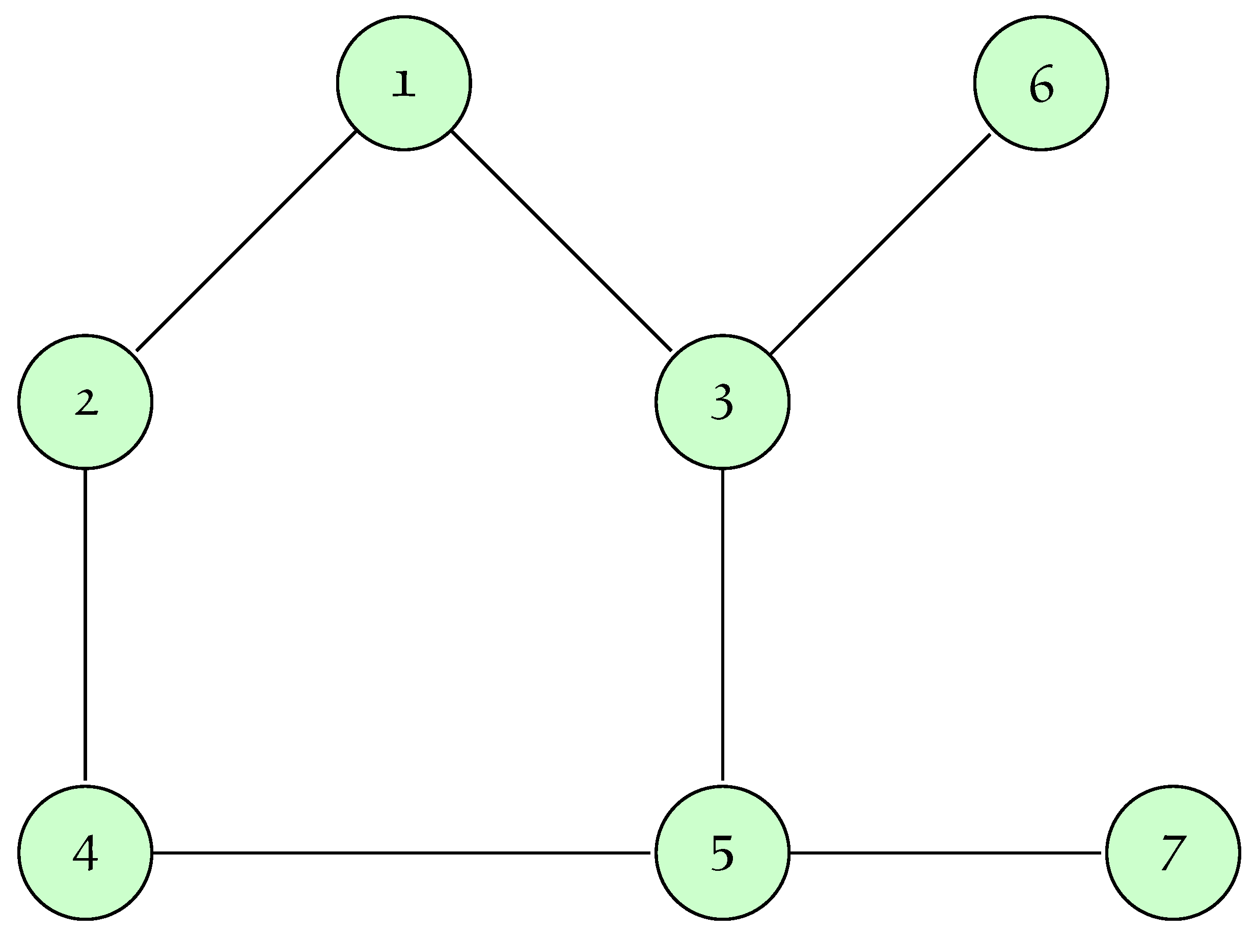
The online SN can be expressed by a weighted spherical linear Diophantine fuzzy graph. Now, we let $\mathfrak{G}=(\mathfrak{V},\mathfrak{E})$ be an undirected SLDFG. We can exemplify an SLDF SN as an undirected spherical linear Diophantine fuzzy relational structure $\mathfrak{G}=(\mathfrak{V},\mathfrak{E})$, where $\mathfrak{V}=\{{\mathfrak{v}}_{\mathfrak{1}},{\mathfrak{v}}_{\mathfrak{2}},{\mathfrak{v}}_{\mathfrak{3}},\dots {\mathfrak{v}}_{\mathfrak{n}}\}$ represents a non-void set of spherical linear Diophantine fuzzy actors or nodes or vertices, and $\mathfrak{E}=\left(\begin{array}{ccc}{\mathfrak{e}}_{\mathfrak{11}}& \cdots & {\mathfrak{e}}_{\mathfrak{1}\mathfrak{n}}\\ ⋮& \ddots & ⋮\\ {\mathfrak{e}}_{\mathfrak{n}\mathfrak{1}}& \cdots & {\mathfrak{e}}_{\mathfrak{nn}}\end{array}\right)$ represents a non-empty set of spherical linear Diophantine fuzzy edges or arcs or a fringe. A small example of a spherical linear Diophantine fuzzy social network is shown in Figure 7. The SN’s nodes and arcs are given in the

Table 7. The node set with SLDFN of graph $\mathfrak{G}$.

Node	SLDFN = $(\langle {\mathfrak{m}}_{\mathfrak{D}},{\mathfrak{a}}_{\mathfrak{D}},{\mathfrak{n}}_{\mathfrak{D}}\rangle ,\langle {\mathit{\alpha }}_{\mathfrak{D}},{\mathit{\beta }}_{\mathfrak{D}},{\mathit{\eta }}_{\mathfrak{D}}\rangle )$
$\mathfrak{1}$	$(\langle 0.7,0.6,0.2\rangle ,\langle 0.3,0.2,0.3\rangle )$
$\mathfrak{2}$	$(\langle 0.6,0.8,0.3\rangle ,\langle 0.3,0.2,0.3\rangle )$
$\mathfrak{3}$	$(\langle 0.7,0.5,0.3\rangle ,\langle 0.4,0.3,0.1\rangle )$
$\mathfrak{4}$	$(\langle 0.5,0.6,0.9\rangle ,\langle 0.2,0.3,0.2\rangle )$
$\mathfrak{5}$	$(\langle 0.8,0.9,0.6\rangle ,\langle 0.1,0.6,0.3\rangle )$
$\mathfrak{6}$	$(\langle 0.3,0.7,0.2\rangle ,\langle 0.6,0.3,0.1\rangle )$
$\mathfrak{7}$	$(\langle 0.3,0.5,0.1\rangle ,\langle 0.5,0.2,0.1\rangle )$

and

Table 8. The arc set with SLDFN of graph $\mathfrak{G}$.

Arc	SLDFN = $(\langle {\mathfrak{m}}_{\mathfrak{D}},{\mathfrak{a}}_{\mathfrak{D}},{\mathfrak{n}}_{\mathfrak{D}}\rangle ,\langle {\mathit{\alpha }}_{\mathfrak{D}},{\mathit{\beta }}_{\mathfrak{D}},{\mathit{\eta }}_{\mathfrak{D}}\rangle )$
${\mathfrak{e}}_{\mathfrak{1}}=\mathfrak{12}$	$(\langle 0.6,0.8,0.3\rangle ,\langle 0.3,0.2,0.3\rangle )$
${\mathfrak{e}}_{\mathfrak{2}}=\mathfrak{13}$	$(\langle 0.7,0.6,0.3\rangle ,\langle 0.3,0.3,0.3\rangle )$
${\mathfrak{e}}_{\mathfrak{3}}=\mathfrak{24}$	$(\langle 0.5,0.8,0.9\rangle ,\langle 0.2,0.3,0.3\rangle )$
${\mathfrak{e}}_{\mathfrak{4}}=\mathfrak{35}$	$(\langle 0.7,0.9,0.6\rangle ,\langle 0.1,0.6,0.3\rangle )$
${\mathfrak{e}}_{\mathfrak{5}}=\mathfrak{36}$	$(\langle 0.3,0.5,0.3\rangle ,\langle 0.4,0.3,0.1\rangle )$
${\mathfrak{e}}_{\mathfrak{6}}=\mathfrak{45}$	$(\langle 0.5,0.9,0.9\rangle ,\langle 0.1,0.6,0.3\rangle )$
${\mathfrak{e}}_{\mathfrak{7}}=\mathfrak{57}$	$(\langle 0.3,0.9,0.6\rangle ,\langle 0.1,0.6,0.3\rangle )$

, respectively.

Arcs are just an absent or present undirected spherical linear Diophantine fuzzy relation with no further information attached for undirected spherical linear Diophantine fuzzy social networks.

We assume that $\mathfrak{G}=(\mathfrak{V},\mathfrak{E})$ is a directed SLDFG. We can exemplify an SLDF SN as a directed spherical linear Diophantine fuzzy relational structure $\mathfrak{G}=(\mathfrak{V},\mathfrak{E})$, where $\mathfrak{V}=\{{\mathfrak{v}}_{\mathfrak{1}},{\mathfrak{v}}_{\mathfrak{2}},{\mathfrak{v}}_{\mathfrak{3}},\dots {\mathfrak{v}}_{\mathfrak{n}}\}$ represents a non-void set of spherical linear Diophantine fuzzy actors or nodes or vertices, and $\mathfrak{E}=\left(\begin{array}{ccc}{\mathfrak{e}}_{\mathfrak{11}}& \cdots & {\mathfrak{e}}_{\mathfrak{1}\mathfrak{n}}\\ ⋮& \ddots & ⋮\\ {\mathfrak{e}}_{\mathfrak{n}\mathfrak{1}}& \cdots & {\mathfrak{e}}_{\mathfrak{nn}}\end{array}\right)$ represents a non-empty set of spherical linear Diophantine fuzzy edges or arcs or a fringe.

In a directed spherical linear Diophantine fuzzy social network, the directed spherical linear Diophantine fuzzy relation is taken into consideration. Because directed spherical linear Diophantine fuzzy relations include more information when arcs are taken into consideration, directed spherical linear Diophantine fuzzy graphs are more effective at modeling social networks. In an undirected spherical linear Diophantine fuzzy social network, the values of ${\mathfrak{e}}_{\mathfrak{ij}}$ and ${\mathfrak{e}}_{\mathfrak{ji}}$ are identical. In the directed spherical linear Diophantine fuzzy social network, however, ${\mathfrak{e}}_{\mathfrak{ij}}$ and ${\mathfrak{e}}_{\mathfrak{ji}}$ are not identical. Figure 8 depicts a miniature version of a directed spherical linear Diophantine fuzzy social network. We let $\mathfrak{G}=(\mathfrak{V},\mathfrak{E})$ be a directed spherical linear Diophantine fuzzy social network. The arc lengths of $\mathfrak{G}$ are described by spherical linear Diophantine fuzzy sets.

The SLDF in-degree centrality (SLDFIDC) of social node ${\mathfrak{v}}_{\mathfrak{i}}$ is the total of the lengths of the arcs that surround it. The following describes the SLDFIDC ${\mathfrak{d}}_{\mathfrak{I}}\left({\mathfrak{v}}_{\mathfrak{i}}\right)$ of node ${\mathfrak{v}}_{\mathfrak{i}}$:

$${\mathfrak{d}}_{\mathfrak{I}}\left({\mathfrak{v}}_{\mathfrak{i}}\right)=\sum _{j=1,j\ne i}^n{\mathfrak{e}}_{\mathfrak{ji}}$$

The SLDF out-degree centrality (SLDFODC) of social node ${\mathfrak{v}}_{\mathfrak{i}}$ is the total of the lengths of the arcs that are near to it. The following describes the SLDFODC ${\mathfrak{d}}_{\mathfrak{O}}\left({\mathfrak{v}}_{\mathfrak{i}}\right)$ of node ${\mathfrak{v}}_{\mathfrak{i}}$:

$${\mathfrak{d}}_{\mathfrak{O}}\left({\mathfrak{v}}_{\mathfrak{i}}\right)=\sum _{j=1,j\ne i}^n{\mathfrak{e}}_{\mathfrak{ji}}$$

In this case, the arc $(i,j)$ is connected to the SLDFS ${\mathfrak{e}}_{\mathfrak{ij}}$, and symbol ∑ represents an addition operation of the SLDFS. Spherical linear Diophantine degree centrality (SLDDC) of node ${\mathfrak{v}}_{\mathfrak{i}}$ is the total of spherical linear Diophantine fuzzy in-degree centrality and spherical linear Diophantine fuzzy out-degree centrality.

$$\mathfrak{d}\left({\mathfrak{v}}_{\mathfrak{i}}\right)={\mathfrak{d}}_{\mathfrak{I}}\left({\mathfrak{v}}_{\mathfrak{i}}\right)\oplus {\mathfrak{d}}_{\mathfrak{O}}\left({\mathfrak{v}}_{\mathfrak{i}}\right)$$

⊕ is an SLDFS addition operation.

We assume that $\mathfrak{G}=(\mathfrak{V},\mathfrak{E})$ is the directed spherical linear Diophantine fuzzy social network of the research team. The collection of seven researchers is represented by $\mathfrak{V}=\{\mathfrak{1},\mathfrak{2},\dots ,\mathfrak{7}\}$ and the directed spherical linear Diophantine fuzzy relation between the seven researchers is represented by the eight-arc set with SLDFN in Table 8. In Figure 8, this social network is displayed. We ascertain the study term’s spherical linear Diophantine fuzzy degree centrality, the spherical linear Diophantine fuzzy out-degree, and the spherical linear Diophantine fuzzy in-degree.

Table 9. Degrees of centrality Table.

Researchers	In-Degree	Out-Degree	Degree of Centrality
$\mathfrak{1}$	$(\langle 0,0,0\rangle ,\langle 0,0,0\rangle )$	$(\langle 0.6,0.8,0.3\rangle ,\langle 0.3,0.3,0.3\rangle )$	$(\langle 0.6,0.8,0.3\rangle ,\langle 0.3,0.3,0.3\rangle )$
$\mathfrak{2}$	$(\langle 0.7,0.6,0.2\rangle ,\langle 0.3,0.2,0.3\rangle )$	$(\langle 0.5,0.6,0.9\rangle ,\langle 0.2,0.3,0.2\rangle )$	$(\langle 0.85,0.36,0.18\rangle ,\langle 0.44,0.06,0.06\rangle )$
$\mathfrak{3}$	$(\langle 0.3,0.7,0.2\rangle ,\langle 0.3,0.3,0.3\rangle )$	$(\langle 0.8,0.9,0.6\rangle ,\langle 0.1,0.6,0.3\rangle )$	$(\langle 0.86,0.63,0.12\rangle ,\langle 0.37,0.18,0.09\rangle )$
$\mathfrak{4}$	$(\langle 0.6,0.8,0.3\rangle ,\langle 0.3,0.2,0.3\rangle )$	$(\langle 0.8,0.9,0.6\rangle ,\langle 0.1,0.6,0.3\rangle )$	$(\langle 0.92,0.72,0.18\rangle ,\langle 0.37,0.12,0.09\rangle )$
$\mathfrak{5}$	$(\langle 0.5,0.6,0.9\rangle ,\langle 0.2,0.3,0.2\rangle )$	$(\langle 0.3,0.5,0.1\rangle ,\langle 0.5,0.2,0.1\rangle )$	$(\langle 0.65,0.3,0.09\rangle ,\langle 0.6,0.06,0.02\rangle )$
$\mathfrak{6}$	$(\langle 0,0,0\rangle ,\langle 0,0,0\rangle )$	$(\langle 0.7,0.5,0.3\rangle ,\langle 0.4,0.3,0.1\rangle )$	$(\langle 0.7,0.5,0.3\rangle ,\langle 0.4,0.3,0.1\rangle )$
$\mathfrak{7}$	$(\langle 0.8,0.9,0.6\rangle ,\langle 0.1,0.6,0.3\rangle )$	$(\langle 0,0,0\rangle ,\langle 0,0,0\rangle )$	$(\langle 0.8,0.9,0.6\rangle ,\langle 0.1,0.6,0.3\rangle )$

displays the three degrees of centrality values. To compare the various degree values, we employ the raking method of spherical linear Diophantine fuzzy sets in

Table 10. Score Table.

Researchers	Score of In-Degree	Score of Out-Degree Score	Score of Degree of Centrality
$\mathfrak{1}$	0	$-0.4$	$-0.4$
$\mathfrak{2}$	0	$-0.65$	$0.315$
$\mathfrak{3}$	$-0.45$	$-0.75$	$0.105$
$\mathfrak{4}$	$-0.35$	$-0.75$	$0.09$
$\mathfrak{5}$	$-0.65$	$-0.05$	$0.39$
$\mathfrak{6}$	0	$-0.05$	$-0.05$
$\mathfrak{7}$	$-0.75$	0	$-0.75$

.

Since the scores of spherical linear Diophantine fuzzy in-degree centralities for Research (Nodes) 1, 2 and 4 have the same values of zero, we find the accuracy values to be the same and the accuracy values are 0, 0.5 and 0.8833, respectively. Hence, Research (Node) 6 has the greatest accuracy value of spherical linear Diophantine fuzzy in-degree centrality according to the ranking of the SLDFS. This indicates that Researcher 4 is more well-liked and has positive relationships with other members of the network. When it comes to spherical linear Diophantine fuzzy out-degree centrality, Node 7 has the highest score value. Hence, we know that a large number of other researchers can be nominated by Node 7. Also, Node 5 has the largest score value in the spherical linear Diophantine fuzzy degree of centrality. Hence, Researcher 5 has a good relationship in all the aspects.

To illustrate a single small social network, we include a straightforward numerical example of a SLDFG in this article. The tiny examples are quite useful in helping to comprehend the benefits of our suggested model. The big data concept and millions of users are the foundation of social networks. As a result, our next task is to use the SLDFG to model a large-scale practical social network and calculate its diameter, closeness, and betweenness. In addition, we present a few heuristic algorithms for determining those metrics for any practical large-scale social network. The suggested model presented in this paper is a significant first addition to SLDFG and social network analysis in an uncertain context, even though more research is required.

6. SLDF Model: Superiority and Applications

Relying on the preceding assertions, computations, and applications, the consequent are the key contingent observations and benefits of employing the concept of T-SFGs and their operations:

(i)

Handling limitations of existing models:

The SLDF model overcomes the limitations of existing models like IFS, PFS, SFSs, and T-SFSs by incorporating control factors. This allows it handling data that violate traditional fuzzy logic constraints, such as the sum of membership grades exceeding one. By introducing control parameters, the SLDF model ensures that the sum remains less than one, making it suitable for scenarios with conflicting attributes and control factors.

(ii)

Flexibility for decision makers:

Unlike existing models that restrict the selection of membership grades, the SLDF model offers greater flexibility. Decision makers can freely choose grades within a closed interval, [0, 1], reflecting the benefits and drawbacks associated with each grade. This freedom allows for more nuanced decision making and better reflects the complexity of real-world situations.

(iii)

Handling counter-factual data:

The proposed graphs and operations within the SLDF framework can effectively handle counter-factual data containing control or reference parameters. This is achieved through the introduction of reference parameters, which act as weights for the chosen membership grades. These weights enable the SLDF model to analyze counter-factual scenarios with greater accuracy and reliability.

(iv)

Advantages over existing approaches:

Table 11. Comparitive Analysis Table.

Approaches	$\mathfrak{m}$	$\mathfrak{a}$	$\mathfrak{n}$	Reference Parameters	Limitations
FG [25]	√	×	×	×	Fuzzy graphs can struggle to represent intricate relationships with multiple dimensions or facets
IFG [30]	√	√	×	×	May not fully capture hesitation or indeterminacy that arises in some real-world scenarios
PFG [39]	√	√	√	×	Cannot handle data when the sum of the grades are more than one
SFG [40,41]	√	√	√	×	Handling the data when the sum of the squares grades are more than one is not possible
T-SFG [45]	√	√	√	×	Reference parameters are not included
SLDFG (Proposed)	√	√	√	√	The increased complexity can be difficult to understand, interpret, and computationally expensive to handle

highlights the key advantages of the SLDF model over existing fuzzy logic approaches.

A few more advantages include:

-

Accommodating control factors: SLDF can handle data that violate traditional fuzzy logic constraints, making it suitable for real-world scenarios.

-

Flexibility in grade selection: Decision makers can freely choose grades within a closed interval, [0, 1], leading to more nuanced decision making.

-

Effective handling of counter-factual data: SLDF can analyze counter-factual scenarios with greater accuracy and reliability due to the introduction of control or reference parameters.

(v)

Applications: The SLDF model has the potential to be applied across various domains, including:

-

Network analysis: Traffic routes, airlines networks, 5G networks, telephone networks, wireless networks, and others can be analyzed and studied using the proposed SLDF framework and methodologies.

-

Decision making: SLDF can be used to make informed decisions in complex situations involving conflicting attributes and control factors.

-

Data analysis: SLDF can help analyze counter-factual data and scenarios with greater accuracy and reliability.

-

Fuzzy logic applications: SLDF can be used in various applications where fuzzy logic is employed, such as machine learning, artificial intelligence, and natural language processing.

Overall, the SLDF model offers a significant advancement over existing fuzzy logic approaches by providing greater flexibility, handling data that violate traditional constraints, and effectively analyzing counter-factual scenarios. This makes it a valuable tool for decision making and data analysis in complex real-world situations.

7. Conclusions

Unveiling the power of SLDFGs offers a transformative approach to modeling real-world systems characterized by ambiguity, imprecision, and inconsistencies. Unlike existing models like PFGs, SFGs, T-SFGs, SLDFGs explicitly address the flexibility gap associated with reference parameters. This enables them to capture a broader range of scenarios and manage their components with greater precision.

The well-defined operations for SLDFGs, including complement, union, and join, facilitate consistent and accurate analysis. Compared to classical extensions of fuzzy graph models, SLDFGs exhibit enhanced comparability, efficiency, flexibility, and, most importantly, precision in formulating complex real-world scenarios.

Furthermore, SLDFGs open up exciting avenues for future research. The concept of energy in SLDFGs and other graph-theoretic features like adjacency matrices, duality, and planarity offer promising avenues for exploration. These advancements can empower us to design more robust and efficient systems across diverse fields like computer networks, database systems, image processing, transportation networks, and large social networks. In the future, we will employ the propose notion in the multi-criteria decision making problem.

Finally, Spherical Linear Diophantine Fuzzy Graphs represent a paradigm shift in uncertainty modeling. Their versatility and accuracy hold immense potential for revolutionizing our understanding and analysis of complex systems, paving the way for a future enriched by deeper insights and transformative applications. In our future work, we will focus on simulation results and formal comparison of results with real problem data as a continuation of the present work.

References

- Zadeh, L.A. Information and control. Fuzzy Sets 1965, 8, 338–353. [Google Scholar] [CrossRef]
- Al-Samarraay, M.; Al-Zuhairi, O.; Alamoodi, A.H.; Albahri, O.S.; Deveci, M.; Alobaidi, O.R.; Kou, G. An integrated fuzzy multi-measurement decision-making model for selecting optimization techniques of semiconductor materials. Expert Syst. Appl. 2024, 237, 121439. [Google Scholar] [CrossRef]
- Gokasar, I.; Pamucar, D.; Deveci, M.; Gupta, B.B.; Martinez, L.; Castillo, O. Metaverse integration alternatives of connected autonomous vehicles with self-powered sensors using fuzzy decision making model. Inf. Sci. 2023, 642, 119192. [Google Scholar] [CrossRef]
- Moslem, S.; Farooq, D.; Esztergr-Kiss, D.; Yaseen, G.; Senapati, T.; Deveci, M. A novel spherical decision-making model for measuring the separateness of preferences for drivers? behavior factors associated with road traffic accidents. Expert Syst. Appl. 2024, 238, 122318. [Google Scholar] [CrossRef]
- Zadeh, L.A. The concept of a linguistic variable and its application to approximate reasoning-I. Inf. Sci. 1975, 8, 199–249. [Google Scholar] [CrossRef]
- Atanassov, K.T. Intuitionistic fuzzy sets. In VII ITKRs Session; Sgurev, V., Ed.; Central Science and Technology Library, Bulgarian Academy of Sciences: Sofia, Bulgaria, 1984. [Google Scholar]
- Atanassov, K.T.; Stoeva, S. Intuitionistic fuzzy sets. In Polish Symposium on Interval & Fuzzy Mathematics; Bulgarian Academy of Sciences: Poznan, Poland, 1983; pp. 23–26. [Google Scholar]
- Atanassov, K.T. Intuitionistic fuzzy sets. Fuzzy Sets Syst. 1986, 20, 87–96. [Google Scholar] [CrossRef]
- Atanassov, K.T. Geometrical interpretation of the elemets of the intuitionistic fuzzy objects. Int. J. Bio-Autom. 2016, 20, S27–S42. [Google Scholar]
- Alshehri, N.; Akram, M. Intuitionistic fuzzy planar graphs. Discret. Dyn. Nat. Soc. 2014, 2014. [Google Scholar] [CrossRef]
- Cuong, B.C. Picture fuzzy sets-first results, part 1. In Preprint of Seminar on Neuro-Fuzzy Systems with Applications; Institute of Mathematics: Hanoi, Vietnam, 2013. [Google Scholar]
- Cuong, B.C. Picture fuzzy sets-first results, part 2. In Preprint of Seminar on Neuro-Fuzzy Systems with Applications; Institute of Mathematics: Hanoi, Vietnam, 2013. [Google Scholar]
- Cuong, B.C.; Kreinovich, V. Picture fuzzy sets-A new concept for computational intelligence problems. In Proceedings of the 3rd World Congress on Information and Communication Technologies, Hanoi, Vietnam, 15–18 December 2013. [Google Scholar]
- Andekah, Z.A.; Naderan, M.; Akbarizadeh, G. Semi-supervised Hyperspectral image classification using spatial-spectral features and superpixel-based sparse codes. In Proceedings of the Iranian Conference of Electrical Engineering, Tehran, Iran, 2–4 May 2017; pp. 2229–2234. [Google Scholar]
- Mahmood, T.; Ullah, K.; Khan, Q.; Jan, N. An approach toward decision-making and medical diagnosis problems using the concept of spherical fuzzy sets. Neural Comput. Appl. 2019, 31, 7041–7053. [Google Scholar] [CrossRef]
- Ullah, K.; Mahmood, T.; Jan, N. Similarity measures for T-spherical fuzzy sets with applications in pattern recognition. Symmetry 2018, 10, 193. [Google Scholar] [CrossRef]
- Riaz, M.; Hashmi, M.R.; Pamucar, D.; Chu, Y.M. Spherical linear Diophantine fuzzy sets with modeling uncertainties in MCDM. Comput. Model. Eng. Sci. 2021, 126, 1125–1164. [Google Scholar] [CrossRef]
- Alshammari, I.; Parimala, M.; Ozel, C.; Riaz, M. Spherical linear Diophantine fuzzy TOPSIS algorithm for green supply chain management system. J. Funct. Spaces 2022, 2022, 3136462. [Google Scholar] [CrossRef]
- Habib, A.; Khan, Z.A.; Riaz, M.; Marinkovic, D. Performance Evaluation of Healthcare Supply Chain in Industry 4.0 with Linear Diophantine Fuzzy Sine-Trigonometric Aggregation Operations. Mathematics 2023, 11, 2611. [Google Scholar] [CrossRef]
- Hashmi, M.R.; Tehrim, S.T.; Riaz, M.; Pamucar, D.; Cirovic, G. Spherical linear diophantine fuzzy soft rough sets with multi-criteria decision making. Axioms 2021, 10, 185. [Google Scholar] [CrossRef]
- Qiyas, M.; Khan, N.; Naeem, M.; Okyere, S. Decision-Making Based on Spherical Linear Diophantine Fuzzy Rough Aggregation Operators and EDAS Method. J. Math. 2023, 2023, 5839410. [Google Scholar] [CrossRef]
- Al-Quran, A. T-spherical linear Diophantine fuzzy aggregation operators for multiple attribute decision-making. AIMS Math. 2023, 8, 12257–12286. [Google Scholar] [CrossRef]
- Jane, J.B.; Ganeshi, E.N. A review on big data with machine learning and fuzzy logic for better decision making. Int. J. Sci. Technol. Res. 2019, 8, 1121–1125. [Google Scholar]
- Yeom, C.U.; Kwak, K.C. A Design and Its Application of Multi-Granular Fuzzy Model with Hierarchical Tree Structures. Appl. Sci. 2023, 13, 11175. [Google Scholar] [CrossRef]
- Kaufmann, A. Introduction a la Theorie des Sousensembles Flous; Massonet Cie: Paris, France, 1973. [Google Scholar]
- Rosenfeld, A. Fuzzy graphs. In Fuzzy Sets and Their Applications to Cognitive and Decision Processes; Tanaka, K., Zadeh, L.A., Fu, K.-S., Eds.; Academic Press: New York, NY, USA, 1975; pp. 77–95. [Google Scholar]
- Mordeson, J.N.; Nair, P.S. Fuzzy Graphs and Fuzzy Hyper Graphs; Physical-Verlag: Heidelberg, Germany, 2001. [Google Scholar]
- Bhattacharya, P. Some remarks on fuzzy graphs. Pattern Recognit. Lett. 1987, 6, 297–302. [Google Scholar] [CrossRef]
- Thirunavukarasu, P.; Suresh, R.; Viswanathan, K.K. Energy of a complex fuzzy graph. Int. J. Math. Sci. Eng. Appl. 2016, 10, 243–248. [Google Scholar]
- Parvathi, R.; Karunambigai, M.G. Intuitionistic fuzzy graphs. In Computational Intelligence, Theory and Applications; Springer: Berlin/Heidelberg, Germany, 2006; pp. 139–150. [Google Scholar]
- Akram, M.; Akmal, R. Operations on intuitionistic fuzzy graph structures. Fuzzy Inf. Eng. 2016, 8, 389–410. [Google Scholar] [CrossRef]
- Akram, M.; Davvaz, B. Strong intuitionistic fuzzy graphs. Filomat 2012, 26, 177–196. [Google Scholar] [CrossRef]
- Karunambigai, M.G.; Akram, M.; Buvaneswari, R. Strong and superstrong vertices in intuitionistic fuzzy graphs. J. Intell. Fuzzy Syst. 2016, 30, 671–678. [Google Scholar] [CrossRef]
- Myithili, K.K.; Parvathi, R.; Akram, M. Certain types of intuitionistic fuzzy directed hypergraphs. Int. J. Mach. Learn. Cybern. 2016, 7, 287–295. [Google Scholar] [CrossRef]
- Nagoorgani, A.; Akram, M.; Anupriya, S. Double domination on intuitionistic fuzzy graphs. J. Appl. Math. Comput. 2016, 52, 515–528. [Google Scholar] [CrossRef]
- Palaniappan, N.; Srinivasan, R. Applications of intuitionistic fuzzy sets of root type in image processing. In Proceedings of the NAFIPS 2009–009 Annual Meeting of the North American Fuzzy Information Processing Society, New York, NY, USA, 1–6 June 2009; pp. 1–5. [Google Scholar]
- Parvathi, R.; Karunambigai, M.G.; Atanassov, K.T. Operations on intuitionistic fuzzy graphs. In Proceedings of the 2009 IEEE International Conference on Fuzzy Systems, Jeju, Republic of Korea, 20–24 August 2009; pp. 1396–1401. [Google Scholar]
- Parvathi, R.; Thamizhendhi, G. Domination in intuitionistic fuzzy graphs. Notes Intuitionistic Fuzzy Sets 2010, 16, 39–49. [Google Scholar]
- Zuo, C.; Pal, A.; Dey, A. New concepts of picture fuzzy graphs with application. Mathematics 2019, 7, 470. [Google Scholar] [CrossRef]
- Akram, M. Decision Making Method Based on Spherical Fuzzy Graphs. In Studies in Fuzziness and Soft Computing; Kahraman, C., Otay, I., Eds.; Springer: Berlin/Heidelberg, Germany, 2020. [Google Scholar]
- Akram, M.; Saleem, D.; Al-Hawary, T. Spherical fuzzy graphs with application to decision-making. Math. Comput. Appl. 2020, 25, 8. [Google Scholar] [CrossRef]
- Hanif, M.Z.; Yaqoob, N.; Riaz, M.; Aslam, M. Linear Diophantine fuzzy graphs with new decision-making approach. AIMS Math. 2022, 7, 14532–14556. [Google Scholar] [CrossRef]
- Parimala, M.; Jafari, S.; Riaz, M.; Aslam, M. Applying the Dijkstra algorithm to solve a linear Diophantine fuzzy environment. Symmetry 2021, 13, 1616. [Google Scholar] [CrossRef]
- Parimala, M.; Prakash, K.; Al-Quran, A.; Riaz, M.; Jafari, S. Optimization Algorithms of PERT/CPM Network Diagrams in Linear Diophantine Fuzzy Environment. Comput. Model. Eng. Sci. 2024, 139, 1095–1118. [Google Scholar] [CrossRef]
- Guleria, A.; Bajaj, R.K. T-spherical fuzzy graphs: Operations and applications in various selection processes. Arab. J. Sci. Eng. 2020, 45, 2177–2193. [Google Scholar] [CrossRef]
- Samanta, S.; Pal, M.A. New approach to social networks based on fuzzy graphs. J. Mass Commun. J. 2014, 5, 078–099. [Google Scholar]
- Fan, T.F.; Liau, C.J.; Lin, T.Y. Positional analysis in fuzzy social networks. In Proceedings of the 2007 IEEE International Conference on Granular Computing (GRC 2007), Fremont, CA, USA, 2–4 November 2007; p. 423. [Google Scholar]
- Kundu, S.; Pal, S.K. Fuzzy granular social networks-model and applications. Inf. Sci. 2015, 314, 100–117. [Google Scholar] [CrossRef]
- Kundu, S.; Pal, S.K. Fuzzy-rough community in social networks. Pattern Recognit. Lett. 2015, 67, 145–152. [Google Scholar] [CrossRef]
- Freeman, L.C. Centrality in social networks conceptual clarification. Soc. Netw. 1978, 1, 215–239. [Google Scholar] [CrossRef]
- Dey, A.; Pal, A. Computing the shortest path with words. Int. J. Adv. Intell. 2019, 12, 355–369. [Google Scholar] [CrossRef]
- Dey, A.; Pradhan, R.; Pal, A.; Pal, T. A genetic algorithm for solving fuzzy shortest path problems with interval type-2 fuzzy arc lengths. Malays. J. Comput. Sci. 2018, 31, 255–270. [Google Scholar] [CrossRef]
Disclaimer/Publisher’s Note: The statements, opinions and data contained in all publications are solely those of the individual author(s) and contributor(s) and not of MDPI and/or the editor(s). MDPI and/or the editor(s) disclaim responsibility for any injury to people or property resulting from any ideas, methods, instructions or products referred to in the content. |
© 2024 by the authors. Licensee MDPI, Basel, Switzerland. This article is an open access article distributed under the terms and conditions of the Creative Commons Attribution (CC BY) license (https://creativecommons.org/licenses/by/4.0/).