On Population Models with Delays and Dependence on Past Values

Abstract

The current values of many populations depend on the past values of the population. In many cases, this dependence is caused by the time certain processes take. This dependence on the past can be introduced into mathematical models by adding delays. For example, the growth rate of a population depends on the population $\tau$ time units ago, where $\tau$ is the maturation time. For an epidemic, there is a time $\tau$ between the contact of an infected individual and a susceptible one, and the time the susceptible individual actually becomes infected. This time $\tau$ is also a delay. So, the number of infected individuals depends on the population at the time $\tau$ units ago. A second way of introducing this dependence on past values is to use non-local operators in the description of the model. Fractional derivatives have commonly been used to provide non-local effects. In population growth models, it can also be done by introducing a new compartment, the immature population, and in epidemic models, by introducing an additional exposed population. In this paper, we study and compare these methods of adding dependence on past values. For models of processes that involve delays, all three methods include dependence on past values, but fractional-order models do not justify the form of the dependence. Simulations show that for the models studied, the fractional differential equation method produces similar results to those obtained by explicitly incorporating the delay, but only for specific values of the fractional derivative order, which is an extra parameter. But in all three methods, the results are improved compared to using ordinary differential equations.

1. Introduction

Many biological processes depend on the population in past times. For a birth process, the number of births depends on the mature population, that is, the population $\tau$ time units ago, with $\tau$ the maturation time of the population. In an epidemic, after contact between a susceptible individual and an infected one, it takes a certain time for the infection-causing agent (virus, bacteria, etc.) to reproduce inside the body and make the individual sick. So, the number of newly infected individuals depends on the number of contacts that occurred at a certain time in the past. At the cell level, immune cells take time to become active and eliminate the bacteria or debris. Of course, not all biological processes depend on the past. For a population with a fixed death rate, the number of deceased individuals at the present time depends only on the number of individuals at the present time. Mathematical models based on ordinary differential equations (ODEs) do not consider the influence of the past. But for models with processes depending on past values, incorporating this dependence into the model equations will change the solutions for the better since the model will be more realistic.

There are three widely used methods for introducing the dependence of a process in the past. The first one is to use delay differential equations (DDEs). The second one is to use fractional differential equations (FDEs). The third one is to introduce additional compartments in the model, where the individuals spend an average time before moving out of the compartment. Introducing delays is a straightforward way of adding the dependence of the past to a biological process. Adding delays may change the dynamics of the process [1,2,3]. Some possible changes are the introduction of oscillations, the introduction of discontinuities in the time derivatives, the non-uniqueness of solutions, and different stability regions. There is a vast amount of literature spanning many years on epidemic or disease transmission models using delay differential equations (DDEs) (see, for example, [1,4,5,6,7,8]). For epidemic models at the population level, the time between a susceptible having contact with an infective and actually getting the disease (time of infection) is the most commonly considered delay. But there are also other delays like maturation times, the time it takes a vaccine to become effective, the time it takes an infected individual to recover after getting the disease, etc. For a within-host infection, delays include the time it takes the pathogen to replicate or reproduce and spread over the affected organ, the time it takes the immune system to react, and the time it takes cells to reproduce, among others. There are different types of delays. Discrete-constant delays are used when each delay has the same value for the entire population. Distributed or continuous delays are used when the delay varies according to a given distribution, such as normal or gamma, around the mean value. In this paper, we will only consider discrete delays. Fractional calculus started with a letter from L’Hôpital to Leibniz asking about derivatives in non-integer order. There are several different definitions for fractional derivatives and integrals, with the most common ones being the Riemann–Liouville and the Caputo versions. There are many good papers and books about differential equations using fractional derivatives (FDEs), such as [9,10,11,12]. In recent years, a vast number of papers have used fractional derivatives in epidemic models, including many for specific epidemics such as influenza, dengue, and COVID-19 [13,14,15,16,17]. The Caputo form is the most widely used fractional derivative. It has the advantages that its derivative of a constant is zero and for FDEs, the initial conditions are given in terms of the unknown and, if necessary, integer-order derivatives at the initial point. Exact solutions of FDEs are hard to find. There are several numerical methods [18,19,20,21]. Fractional derivatives are non-local operators that involve the solution from the initial time until the current time. So, the solution at the current time depends on the solution at all previous times, so FDEs incorporate memory. ODEs neglect such effects. In addition, when fitting data, fractional models have more degrees of freedom through the orders of the fractional derivatives compared to ODE models. In fact, many papers that use fractional derivative models for epidemics justify their use by demonstrating superior data fitting compared to ordinary differential equation models. This has been done for different epidemics such as dengue, Ebola, and COVID-19 [14,22,23]. Discrete-time fractional differential equations have also been used [24,25,26] but not as widely as continuous-time fractional differential equations. Possible reasons for this are that popular methods become more popular and the widespread availability of ready-to-use software for FDEs. A third way of introducing dependence on the past in a population mathematical model is to add more compartments. For models including birth processes, this can be achieved by adding an immature population, with individuals staying in this compartment for an average time equal to the maturation period. Examples involving insect populations can be found in [27,28]. In epidemic models, this can be achieved by adding an exposed population [29,30,31]. The dependence of solutions on past values is a topic of very high interest, especially in epidemics, with some recent references being [32,33,34,35,36]. The main objective of this paper is to study how to introduce dependence on past values into ordinary differential models of population growth and disease transmission. This is discussed in Section 2. In Section 3, results and numerical simulations are presented. Finally, in Section 4, a discussion of the results is presented.

2. Materials and Methods

In this section, we present the addition of dependence on the past using delays, fractional derivatives, and additional compartments to several compartmental models of population growth, epidemics, and within-host infection propagation.

We start with very simple models and continue to more complicated ones. For all examples, dependence on the past is added to the ODE model using three methods. The first method is to introduce discrete delays. While this can be done in several ways, not all of them make biological sense. The second method is to use non-local fractional derivatives instead of time derivatives. The third method is to add more population compartments, such as immature or exposed populations, and incorporate dependence on the past based on the time individuals spend in these compartments. For the simplest model considered, with one population and described by a linear differential equation, it is possible to calculate exact solutions for the original ODE and all models based on the three methods. For the delay differential equation models, the solution requires numerical approximation of the solution of a transcendental equation. For the logistic model, there is an exact solution only for the ODE, but stability can be found for all models. For the epidemic models, there are no exact solutions, and the local asymptotic stability of the disease-free equilibrium can be determined for all methods. But the expressions become more complicated with the complexity of the model.

The pyramid flowchart depicted in Figure 1 illustrates the sequence of models used in this paper. These models progress from linear, with one state given by the Malthus model, to non-linear, with one state given by the logistic model, and finally, to non-linear epidemic models with several states, each increasing in complexity. ODE refers to the corresponding ordinary differential equations model, DDE refers to the delay differential equations model, EXP refers to the model with immature or exposed populations, and FRAC refers to the fractional differential equations model. E indicates that the model has an exact solution, S indicates the local asymptotic stability of the steady states for the Malthus and logistic models, and of the disease-free equilibrium for the infection models. These results are shown later in this section. In Section 3, the simulations show that all methods that incorporate dependence on the past can produce similar results, except for the fractional derivative equations models, where this holds true only for specific values of the fractional order.

2.1. Population Growth Models

Many mathematical population models can be derived by starting with a discrete-time population model [37,38]. All these models state that the current population is equal to the population at the previous time plus its change during the time step. For example, for a model considering only birth and death processes, the population at time $t+\Delta t$ can be given as the population at time t plus the new births minus the new deaths. The discrete-time model is

$$N(t+\Delta t)=N\left(t\right)+\Delta tbN\left(t\right)-\Delta t\mu N\left(t\right),$$

where $N\left(t\right)$ is the population at time t, $b>0$ is the birth rate, and $\mu >0$ is the death rate. By taking the limit as $\Delta t$ tends to 0, we obtain the simplest continuous-time population model known as the Malthus model

$$\frac{dN}{dt}=(b-\mu )N\left(t\right).$$

(1)

For many populations, there is a delay $\tau >0$ due to the maturation time in the birth process. But the number of deaths depends only on the current population. By adding a delay to the discrete-time model, we obtain

$$N(t+\Delta t)=N\left(t\right)+\Delta tbN(t-k\Delta t)-\Delta t\mu N\left(t\right),$$

where the delay is $\tau =k\Delta t$, with k being a positive integer. Again, taking the limit as $\Delta t$ tends to 0 and keeping $k\Delta t$ constant, we obtain the delayed continuous-time model

$$\frac{dN}{dt}=bN(t-\tau )-\mu N\left(t\right)$$

(2)

that takes into consideration the maturation time. The Malthus model and the delayed Malthus model have only one equilibrium point, $N\left(t\right)=0$. One issue with using the DDE model is that it requires initial values on the history interval $[t_0-\tau ,t_0]$, where $t_0$ is the initial time.

Instead of having a single value, the maturation time may take values in an interval $[k_i\Delta t,k_f\Delta t]$, where $0\le k_i\le k_f$. The model is

$$N(t+\Delta t)=N\left(t\right)+\Delta tb\sum _{k=k_i}^{k_f}G(t-k\Delta t)N(t-k\Delta t)-\Delta t\mu N\left(t\right),$$

(3)

where $G(t-k\Delta t)$ is a weighting function with an average of one.

By taking the limit as $\Delta t$ tends to 0 and keeping the terms $k\Delta t$ constant, $k=k_i,\dots ,k_f$, one obtains the distributed delay equation

$$\frac{dN}{dt}={\int }_{-\infty }^{t}G(t-s)bN(t-s)ds-\mu N\left(t\right).$$

The function G is taken to have compact support and an average of 1. Usually, it has a very small support. For a discrete delay, it is taken as a Dirac delta function. The birth function $bN$ can be replaced with another birth function or with a function F representing other processes happening in the past. Also, the death term $\mu N$ can be substituted with a function H representing all the processes happening at the present time. A more general integro-differential equation for the growth of one population can be written as

$$\frac{dN}{dt}={\int }_{-\infty }^{t}G(t-s)F\left(N(t-s)\right)ds-H\left(N\left(t\right)\right).$$

(4)

A discrete-time model that considers an immature population is

$$\begin{array}{cc}\hfill N(t+\Delta t)& =N\left(t\right)+\Delta t\sigma Y\left(t\right)-\Delta t\mu N\left(t\right)\hfill \\ \hfill Y(t+\Delta t)& =Y\left(t\right)+bN\left(t\right)-\Delta t\mu Y\left(t\right)-\Delta t\sigma Y\left(t\right),\hfill \end{array}$$

where $Y\left(t\right)$ is the immature or young population, all new births are immature, and $\sigma =1/\tau$ is the rate at which the immature population matures. Taking the limit as $\Delta t$ tends to 0, we obtain the ODE model that consists of a system of equations for the two age groups, mature, N, and immature, Y [27,28],

$$\begin{array}{cc}\hfill \frac{dN}{dt}& =\sigma Y-\mu N\hfill \\ \hfill \frac{dY}{dt}& =bN-\sigma Y-\mu Y.\hfill \end{array}$$

(5)

A modification of Malthus’s continuous-time model using fractional derivatives is introduced later in this subsection.

A second population growth model that adds intra-species competition for resources is the logistic growth model given by

$$\frac{dN}{dt}=rN\left(t\right)(1-\frac{N\left(t\right)}{K}),$$

(6)

where $N\left(t\right)$ is the population, $r=b-\mu$ is the growth rate, and K is the carrying capacity.

The maturation time delay can again be introduced into the birth term:

$$\frac{dN}{dt}=bN(t-\tau )-r\frac{N{\left(t\right)}^2}{K}-\mu N\left(t\right).$$

(7)

The competition and death terms depend on the current time t. One disadvantage of delay differential equations is that they require initial conditions given on the interval $[t_0-\tau ,t_0]$, where $t_0$ is the initial time. This interval is usually called the history interval.

Following the approach used in the Malthus model, an alternative way of adding dependence on the past is to introduce an immature population

$$\begin{array}{cc}\hfill \frac{dN}{t}& =\sigma Y-r{N}^2/K-\mu N\hfill \\ \hfill \frac{dY}{dt}& =bN-r{Y}^2/K-\sigma Y-\mu Y,\hfill \end{array}$$

(8)

where $r=b-\mu$ and $\sigma$ is 1 over the maturation time. We assume that there is no competition between the adult and the immature populations, as is the case for insects, where the larvae feed on different food than the adults. But there are several other ways of introducing the immature population.

Before writing the model using FDEs, we introduce some definitions. The Caputo fractional derivative, which is now the most commonly used fractional operator in mathematical biology models, is obtained by modifying the definition of the Riemann–Liouville fractional derivative to regularize the initial conditions, so they are stated only in terms of ordinary derivatives [9,10]. In our definitions of Riemann–Liouville and Caputo fractional derivatives, we consider that the initial time is $t=0$. The Riemann–Liouville fractional derivative is

$${}_0{}^R{D}_t^{\alpha }y\left(t\right)=\frac{1}{\mathsf{\Gamma }(m-\alpha )}\frac{d^m}{d{t}^m}{\int }_0^t{(t-\tau )}^{-\alpha -1+m}y\left(\tau \right)d\tau ,m-1<\alpha <m,$$

and the Caputo fractional derivative is

$${}_0{}^C{D}_t^{\alpha }y\left(t\right)=\frac{1}{\mathsf{\Gamma }(m-\alpha )}{\int }_0^t{(t-\tau )}^{-\alpha -1+m}\frac{d^m}{d{\tau }^m}y\left(\tau \right)d\tau ,m-1<\alpha <m,$$

(9)

where $\alpha$ is the order of the derivative. These two definitions are not equivalent to each other. Their difference is expressed by

$${}_0{}^C{D}_t^{\alpha }y\left(t\right)={}_0{}^R{D}_t^{\alpha }y\left(t\right)-\sum _{\nu =0}^{m-1}{r}_{\nu }^{\alpha }\left(t\right)y^{\left(\nu \right)}\left(0\right),r_{\nu }^{\alpha }\left(t\right)=\frac{t^{\nu -\alpha }}{\mathsf{\Gamma }(\nu +1-\alpha )}.$$

The Caputo operator ${}_0{}^C{D}_t^{\alpha }$ has the advantage for differential equations with initial values in that these initial values are given in terms of ordinary derivatives. The initial values for Caputo differential equations are given as

$${}_0{}^C{D}_t^{\alpha }y\left(0\right)=b_{\nu },\nu =1,2,\dots m,$$

with $m-1<\alpha \le m$. In our examples, $m=1$. From the definition of the Caputo derivative, ${}_0{}^C{D}_t^{\alpha }y\left(t\right)$, it can be seen that it is a non-local operator over the interval $(0,t)$ and that it does not depend on values for $t<0$. From the kernel of the integral, it is clear that it is weighted toward the values of $y\left(t\right)$ at time t. The replacement of the integer-order derivative with a fractional-order one in population models is usually justified by stating that the population has memory, that is, it depends on the past. But it is not stated how it takes into account the actual dependence on the past and whether it is due to maturation or infection times, or to other processes.

Another definition of the fractional derivative $D_t^{\alpha }y\left(t\right)$, the Grünwald–Letnikov definition, is based on taking finite differences on equidistant time steps in $[0,t]$. Choose the grid

$$0=t_0<t_1<\dots <t=t_{n+1}=(n+1)\Delta t,t_{n+1}-t_n=\Delta t,$$

and use the usual notation of finite differences,

$$\frac{1}{\Delta t^{\alpha }}{\Delta }_{\Delta t}^{\alpha }y\left(t\right)=\frac{1}{\Delta t^{\alpha }}\left(y\left(t_{n+1}\right)-\sum _{\nu =1}^{n+1}{c}_{\nu }^{\alpha }y\left(t_{n+1-\nu }\right)\right),$$

where

$$c_{\nu }^{\alpha }={(-1)}^{\nu -1}\left(\genfrac{}{}{0pt}{}{\alpha }{\nu }\right).$$

Then, the Grünwald–Letnikov definition is [9,19]

$$D_t^{\alpha }y\left(t\right)=\underset{\Delta t\to 0}{lim}\frac{1}{\Delta t^{\alpha }}{\Delta }_{\Delta t}^{\alpha }y\left(t\right).$$

Take the limit $\alpha \to 1$ to obtain the explicit or implicit Euler method. Compared with linear multistep methods for the approximation of the fractional derivative, the sum of divided differences becomes longer and longer [9,19], so it is not usually used in practice. But it is useful for comparing an approximation of a fractional differential equation to that of an ODE. We apply the Grünwald–Letnikov definition to the following fractional differential equation

$${}_0{}^C{D}_t^{\alpha }N\left(t\right)=f\left(N\left(t\right)\right),N\left(0\right)=N_0(0<\alpha <1),$$

and let $N\left(t\right)$ be the exact solution in the interval $[0,T]$. If $N_k$ denotes the approximation of the true solution $N\left(t_k\right)$, then the explicit or implicit Grünwald–Letnikov method on a uniform grid is given by

$$N_{n+1}-\sum _{\nu =1}^{n+1}{c}_{\nu }^{\alpha }{N}_{n+1-\nu }-r_{n+1}^{\alpha }{N}_0=\Delta t^{\alpha }f\left(N_n\right)\mathrm{or}\Delta t^{\alpha }f\left(N_{n+1}\right).$$

Here, $r_{n+1}^{\alpha }=\frac{{(n+1)}^{-\alpha }}{\mathsf{\Gamma }(1-\alpha )}$, with $\mathsf{\Gamma }$ the Gamma function. Taking $n=0$, the equation for the first step is

$$N_1-c_1^{\alpha }{N}_0-r_1^{\alpha }{N}_0=\Delta t^{\alpha }f\left(N_0\right)\mathrm{or}\Delta t^{\alpha }f\left(N_1\right).$$

This equation does not agree with the first step of any standard finite approximation of Equation (3). The Caputo derivative incorporates past values of the solution starting at the initial time $t=0$, but it also has terms that do not come from a standard discrete-time conservation equation. The population Malthus growth model in terms of Caputo fractional derivatives is

$${}_0{}^C{D}_t^{\alpha }N\left(t\right)=(b-\mu )N\left(t\right).$$

(10)

2.2. SIRS Models

A model commonly used for the propagation of many different diseases in a population is the SIRS model with no demographics [37]. It consists of three compartments: susceptibles ($S\left(t\right)$), infectives or infected ($I\left(t\right)$), and recovered ($R\left(t\right)$). A susceptible turns into an infective with a given probability after contact with an infective. An infective recovers with a rate $\gamma$. A recovered loses immunity at a rate $\nu$ and converts into a susceptible. The total population is assumed constant, $S\left(t\right)+I\left(t\right)+R\left(t\right)=N$, and the disease is assumed to be short enough so that births and deaths need not be considered. The infection coefficient is denoted by $\beta /N$. All parameters are positive. The system of ordinary differential equations (ODEs) describing the model is

$$\begin{array}{cc}\hfill \frac{dS}{dt}& =-\frac{\beta }{N}SI+\nu R\hfill \\ \hfill \frac{dI}{dt}& =\frac{\beta }{N}SI-\gamma I\hfill \\ \hfill \frac{dR}{dt}& =\gamma I-\nu R.\hfill \end{array}$$

(11)

Since the total population is constant, one equation can be eliminated using $R\left(t\right)=N-S\left(t\right)-I\left(t\right)$. The new system of equations is

$$\begin{array}{cc}\hfill \frac{dS}{dt}& =-\frac{\beta }{N}SI+\nu (N-S-I)\hfill \\ \hfill \frac{dI}{dt}& =\frac{\beta }{N}SI-\gamma I.\hfill \end{array}$$

This continuous-time model can also be derived from a discrete-time model [39,40].

There are several different methods of introducing delays in the infection into the model. The first one, which we call SIRS Model 1 [41,42,43], is given by

$$\begin{array}{cc}\hfill \frac{dS}{dt}& =-\frac{\beta }{N}S(t-\tau )I(t-\tau )+\nu (N-S\left(t\right)-I\left(t\right))\hfill \\ \hfill \frac{dI}{dt}& =\frac{\beta }{N}S(t-\tau )I(t-\tau )-\gamma I\left(t\right),\hfill \end{array}$$

(12)

where the hypothesis is that an infective has contact with a susceptible and it takes time $\tau$ for this susceptible to turn infective. Until that time, it is counted as a susceptible. The second model is SIRS Model 2 [44], which is described by

$$\begin{array}{cc}\hfill \frac{dS}{dt}& =-\frac{\beta }{N}S\left(t\right)I(t-\tau )+\nu (N-S\left(t\right)-I\left(t\right))\hfill \\ \hfill \frac{dI}{dt}& =\frac{\beta }{N}S\left(t\right)I(t-\tau )-\gamma I\left(t\right),\hfill \end{array}$$

(13)

where the assumption is that after contact between a susceptible and an infective, time $\tau$ has to pass before the susceptible turns into an infective and is able to infect another susceptible. So, there is a new infective after contact between the susceptible and an individual infected a time ago equal to the delay.

The third model is SIRS Model 3, which is described by

$$\begin{array}{cc}\hfill \frac{dS}{dt}& =-\frac{\beta }{N}S\left(t\right)I\left(t\right)+\nu (N-S\left(t\right)-I\left(t\right))\hfill \\ \hfill \frac{dI}{dt}& =\frac{\beta }{N}S(t-\tau )I(t-\tau )-\gamma I\left(t\right),\hfill \end{array}$$

(14)

where after contact with an infective, the susceptible leaves the susceptible population but takes time $\tau$ to be included in the infective population. It conserves the total population, and the infection contact is between individuals at the same time. These three models can all be derived from discrete-time models.

As shown in [45], temporary immunity can be included in the SIRS model. The authors used a distributed delay, but by introducing the delay after exposure ${\tau }_1$, the delay due to the minimum duration of the disease ${\tau }_2$, and the delay due to the minimum time with immunity ${\tau }_3$, we obtain the model

$$\begin{array}{cc}\hfill \frac{dS}{dt}& =-\frac{\beta }{N}S(t-{\tau }_1)I(t-{\tau }_1)+\nu R(t-{\tau }_3)\hfill \\ \hfill \frac{dI}{dt}& =\frac{\beta }{N}S(t-{\tau }_1)I(t-{\tau }_1)-\gamma I(t-{\tau }_2)\hfill \\ \hfill \frac{dR}{dt}& =\gamma I(t-{\tau }_2)-\nu R(t-{\tau }_3).\hfill \end{array}$$

These are the equations for SIRS Model 1, but the equations for SIRS Models 2 and 3 are similar.

Models with delays introduced in different forms may have the same equilibrium solutions but the actual time-dependent solutions will be different. There is also the question of the influence of the initial conditions given in the history interval. For an epidemic, they can always be given as the equilibrium solutions with no disease. That is, the natural assumption that the epidemic starts at $t=0$ can be used.

The SIRS fractional model is

$$\begin{array}{cc}\hfill {}_0{}^C{D}_t^{\alpha }S\left(t\right)& =-\frac{\beta }{N}SI+\nu R\hfill \\ \hfill {}_0{}^C{D}_t^{\alpha }I\left(t\right)& =\frac{\beta }{N}SI-\gamma I\hfill \\ \hfill {}_0{}^C{D}_t^{\alpha }R\left(t\right)& =\gamma I-\nu R.\hfill \end{array}$$

(15)

The same fractional order, $\alpha$, was used for all three fractional derivatives. This is not necessary but is usually done for fractional epidemic models [13,14,46]. Two examples of papers using different orders are [22,47]. These fractional derivative models include dependence on all population values between the initial and the current times, but, again from looking at finite difference approximations, they do not arise from standard discrete-time models. But simulations may produce good agreement with real data due to the extra parameters, the fractional derivative orders.

A model that takes into account dependence on the past caused by the delay in transmission by including an exposed population, $E\left(t\right)$, is

$$\begin{array}{cc}\hfill \frac{dS}{dt}& =-\frac{\beta }{N}SI+\nu R\hfill \\ \hfill \frac{dE}{dt}& =\frac{\beta }{N}SI-\sigma E\hfill \\ \hfill \frac{dI}{dt}& =\sigma E-\gamma I\hfill \\ \hfill \frac{dR}{dt}& =\gamma I-\nu R.\hfill \end{array}$$

(16)

The additional parameter is $\sigma =1/\tau$. Models of this form are usually called SEIRS models, and the dependence on the past comes from the average time an individual spends in the exposed compartment.

2.3. Plant Virus with Vector Transmission Models

Humans, animals, and plants can all be affected by vector-transmitted viruses. The processes involved are the same. For simplicity, we consider a model for cultivated plants, for which it is reasonable to assume a constant plant population since farmers replace dead plants. Two examples of virus-causing diseases in plants are the cassava virus [48] and the cacao swollen shoot virus [49]. Again, we introduce the delay in different ways to see the differences in the solutions. We consider a simple model with two populations of plants: susceptible (healthy), $S\left(t\right)$, and infective (already infected), $I\left(t\right)$. Usually, plants do not recover so we do not consider a recovered class. There are also two populations of vectors: susceptible, $X\left(t\right)$, and infective, $Y\left(t\right)$. Vectors are only carriers and do not get the disease so they do not recover. A susceptible plant becomes infected when an infected vector feeds on it, and a susceptible vector becomes infected by feeding on an infected plant. This model is a simplified version of the models presented, for example, in [43,50].

The assumptions of the model are as follows: all new plants and vectors are susceptible; the total population of plants is a constant K; the infection terms between vectors and plants, and vice versa, are of mass-action type; the viruses only kill plants; and neither plants nor vectors recover from the disease.

The system of ODEs for the model is

$$\begin{array}{cc}\hfill \frac{dS}{dt}& =\mu (K-S)+dI-\beta YS\hfill \\ \hfill \frac{dI}{dt}& =\beta YS-(d+\mu )I\hfill \\ \hfill \frac{dX}{dt}& =\mathsf{\Lambda }-{\beta }_{1}IX-mX\hfill \\ \hfill \frac{dY}{dt}& ={\beta }_{1}IX-mY.\hfill \end{array}$$

(17)

The parameters of the model are taken from [43,50] and are all positive: K is the total number of plants, $\beta$ is the infection rate of plants due to infective vectors feeding on the plant and infecting it, ${\beta }_1$ is the infection rate of vectors due to feeding on an infected plant and becoming infected, $\mu$ is the natural death rate of plants, d is the additional death rate of plants due to the disease, m is the natural death rate of vectors, and $\mathsf{\Lambda }$ is the replenishing rate of vectors (due to birth and/or migration).

In this virus transmission via a vector model, there are two delays. The first one is the time it takes the virus to spread in the plant after infected contact. The second one is the time it takes the virus to spread in the vector after becoming infected through feeding. Since the virus usually stays around the feeding organs of the vector and does not replicate inside it, this second delay is much smaller than the first. For simplicity, we consider only the first delay.

Following the approach used in the SIRS model, we introduce the delay in the transmission in two different ways. The first one uses the assumption that after contact with an infective, a susceptible takes the delay time to become infective itself [42,43]. That is, a newly exposed susceptible remains a susceptible until a time equal to the delay elapses and only then does it become an infective. This is known as Model A1:

$$\begin{array}{cc}\hfill \frac{dS}{dt}& =\mu (K-S(t\left)\right)+dI\left(t\right)-\beta Y(t-\tau )S(t-\tau )\hfill \\ \hfill \frac{dI}{dt}& =\beta Y(t-\tau )S(t-\tau )-(d+\mu )I\left(t\right)\hfill \\ \hfill \frac{dX}{dt}& =\mathsf{\Lambda }-{\beta }_{1}I\left(t\right)X\left(t\right)-mX\left(t\right)\hfill \\ \hfill \frac{dY}{dt}& ={\beta }_{1}I\left(t\right)X\left(t\right)-mY\left(t\right).\hfill \end{array}$$

(18)

The second model with infection delay uses the assumption that after a contagion, the susceptible immediately stops being susceptible but it takes the delay time to become infective. It takes into account the probability of the newly infected plant dying before becoming infective using the term $exp(-\mu \tau )$, which is the average survival percentage in the time period $\tau$. This is known as Model A2:

$$\begin{array}{cc}\hfill \frac{dS}{dt}& =\mu (K-S(t\left)\right)+dI\left(t\right)-\beta Y\left(t\right)S\left(t\right)\hfill \\ \hfill \frac{dI}{dt}& =exp(-\mu \tau )\beta Y(t-\tau )S(t-\tau )-(d+\mu )I\left(t\right)\hfill \\ \hfill \frac{dX}{dt}& =\mathsf{\Lambda }-{\beta }_{1}I\left(t\right)X\left(t\right)-mX\left(t\right)\hfill \\ \hfill \frac{dY}{dt}& ={\beta }_{1}I\left(t\right)X\left(t\right)-mY\left(t\right).\hfill \end{array}$$

(19)

Delay differential equations, while more realistic, have the drawback that it is necessary to specify initial conditions over an interval instead of just at a point, as with ordinary differential equations. These initial conditions may be unknown, and, if so, are usually assumed to be constant. What is more, they are usually assumed to represent disease-free values. A second drawback is that the analysis is much harder due to the infinite number of eigenvalues [1,51].

A common alternative is to use fractional derivatives, which have their own advantages and difficulties, as already mentioned for the population growth models and the SIRS models. The DFE model is

$$\begin{array}{cc}\hfill {}_0{}^C{D}_t^{\alpha }S\left(t\right)& =\mu (K-S(t\left)\right)+dI\left(t\right)-\beta Y\left(t\right)S\left(t\right)\hfill \\ \hfill {}_0{}^C{D}_t^{\alpha }I\left(t\right)& =\beta Y\left(t\right)S\left(t\right)-(d+\mu )I\left(t\right)\hfill \\ \hfill {}_0{}^C{D}_t^{\alpha }X\left(t\right)& =\mathsf{\Lambda }-{\beta }_{1}I\left(t\right)X\left(t\right)-mX\left(t\right)\hfill \\ \hfill {}_0{}^C{D}_t^{\alpha }Y\left(t\right)& ={\beta }_{1}I\left(t\right)X\left(t\right)-mY\left(t\right).\hfill \end{array}$$

(20)

A third alternative for accounting for dependence on the past is to introduce another compartment, the exposed population (E). After contact with an infective, a susceptible is converted into an exposed or latent, one that cannot yet infect. The exposed turns into an infective at a rate of $ϵ=1/\tau$. The model is

$$\begin{array}{cc}\hfill \frac{dS}{dt}& =\mu (K-S(t\left)\right)+dI\left(t\right)-\beta Y\left(t\right)S\left(t\right)+\mu E\hfill \\ \hfill \frac{dE}{dt}& =\beta Y\left(t\right)S\left(t\right)-\mu E-ϵE\hfill \\ \hfill \frac{dI}{dt}& =ϵE-(d+\mu )I\left(t\right)\hfill \\ \hfill \frac{dX}{dt}& =\mathsf{\Lambda }-{\beta }_{1}I\left(t\right)X\left(t\right)-mX\left(t\right)\hfill \\ \hfill \frac{dY}{dt}& ={\beta }_{1}I\left(t\right)X\left(t\right)--mY\left(t\right).\hfill \end{array}$$

(21)

Epidemic models with an exposed class are very common (for plant virus propagation, see, for example, [30,52]). The advantages of using models with exposed populations are that they are based on ODEs, so they only require the initial condition at the initial time, and, as with all epidemic models based on ODEs, the local asymptotic stability at the beginning of the epidemic can be determined using the next-generation matrix method [53,54]. But, from a biological point of view, there is the complication that an individual only stays in the exposed state for a time equal to the delay, whereas some individuals may stay in this state for a much longer time.

2.4. Within-Host Virus Infection Models

A basic model of within-host virus infection considers three populations: susceptible cells, infected cells, and virus particles (virions). Susceptible cells are recruited and die naturally, and they can become infected through contact with a virus particle. Cells infected with a virus burst and release a certain number of virions. These free virions can infect healthy cells or die. More realistic models also include the elimination of infected cells and virions by the effector cells of the immune system, as well as cell-to-cell transmission. The equations for such models are [55,56,57,58]

$$\begin{array}{cc}\hfill \frac{dx}{dt}& =\lambda -{\mu }_{x}x-\beta xv-{\beta }_{xy}xy\hfill \\ \hfill \frac{dy}{dt}& =\beta xv+{\beta }_{xy}xy-{\beta }_{ey}ye-{\mu }_{y}y\hfill \\ \hfill \frac{dv}{dt}& =B{\mu }_{y}y-\beta xv-{\beta }_{ev}ve-{\mu }_{v}v\hfill \\ \hfill \frac{de}{dt}& =s+{\alpha }_{1}y-{\beta }_{ye}ye-{\beta }_{ve}ve-{\mu }_{e}e.\hfill \end{array}$$

(22)

Here, $x,y$, v, and e are the concentrations of susceptible cells, infected cells, virions, and effector cells, respectively. $\lambda$ is the recruitment rate of new susceptible cells, ${\mu }_x$ is their death rate, $\beta$ is the infection rate, ${\mu }_y$ is the killing rate of infected cells by the virus, B is the number of virions produced per infected cell, and ${\mu }_v$ is the death rate of virions. Susceptible cells can be infected through direct contact with an infected cell at a rate ${\beta }_{xy}$; effector cells eliminate infected cells at a rate ${\beta }_{ey}$; free virus particles are introduced into susceptible cells at a rate $\beta$; and effector cells are recruited at a constant rate s and are also recruited depending on the number of infected cells y at a rate ${\alpha }_1$. In addition, as effector cells eliminate infected cells and virus particles, they are also eliminated from the system with rates ${\beta }_{ye}$ and ${\beta }_{ve}$, respectively. Finally, effector cells die naturally at a rate ${\mu }_e$. All parameters are non-negative.

We add two delays to the model (22), ${\tau }_1$, which is the time it takes the virus to replicate after invading a cell, and ${\tau }_2$, which is the time it takes the immune system to recruit an effector cell after detecting an infected cell. The delay model is

$$\begin{array}{cc}\hfill \frac{dx}{dt}& =\lambda -{\mu }_{x}x\left(t\right)-\beta x(t-{\tau }_1)v(t-{\tau }_1)-{\beta }_{xy}x(t-{\tau }_1)y(t-{\tau }_1)\hfill \\ \hfill \frac{dy}{dt}& =\beta x(t-{\tau }_1)v(t-{\tau }_1)+{\beta }_{xy}x(t-{\tau }_1)y(t-{\tau }_1)-{\beta }_{ey}y\left(t\right)e\left(t\right)-{\mu }_{y}y\left(t\right)\hfill \\ \hfill \frac{dv}{dt}& =B{\mu }_{y}y\left(t\right)-\beta xv-{\beta }_{ev}v\left(t\right)e\left(t\right)-{\mu }_{v}v\left(t\right)\hfill \\ \hfill \frac{de}{dt}& =s+{\alpha }_{1}y(t-{\tau }_2)-{\beta }_{ye}y\left(t\right)e\left(t\right)-{\beta }_{ve}v\left(t\right)e\left(t\right)-{\mu }_{e}e\left(t\right).\hfill \end{array}$$

(23)

The fractional derivative system is

$$\begin{array}{cc}\hfill {}_0{}^C{D}_t^{\alpha }x\left(t\right)& =\lambda -{\mu }_{x}x\left(t\right)-\beta x\left(t\right)v\left(t\right)-{\beta }_{xy}x\left(t\right)y\left(t\right)\hfill \\ \hfill {}_0{}^C{D}_t^{\alpha }y\left(t\right)& =\beta x\left(t\right)v\left(t\right)+{\beta }_{xy}x\left(t\right)y\left(t\right)-{\beta }_{ey}y\left(t\right)e\left(t\right)-{\mu }_{y}y\left(t\right)\hfill \\ \hfill {}_0{}^C{D}_t^{\alpha }v\left(t\right)& =B{\mu }_{y}y\left(t\right)-\beta xv-{\beta }_{ev}v\left(t\right)e\left(t\right)-{\mu }_{v}v\left(t\right)\hfill \\ \hfill {}_0{}^C{D}_t^{\alpha }e\left(t\right)& =s+{\alpha }_{1}y\left(t\right)-{\beta }_{ye}y\left(t\right)e\left(t\right)-{\beta }_{ve}v\left(t\right)e\left(t\right)-{\mu }_{e}e\left(t\right).\hfill \end{array}$$

(24)

And the model with an exposed cell population z is

$$\begin{array}{cc}\hfill \frac{dx}{dt}& =\lambda -m{u}_{x}x\left(t\right)-\beta x\left(t\right)v\left(t\right)-{\beta }_{xy}x\left(t\right)y\left(t\right)\hfill \\ \hfill \frac{dz}{dt}& =\beta x\left(t\right)v\left(t\right)+{\beta }_{xy}x\left(t\right)y\left(t\right)-{\mu }_{x}z\left(t\right)-\sigma z\left(t\right)\hfill \\ \hfill \frac{dy}{dt}& =\sigma z\left(t\right)-{\beta }_{ey}y\left(t\right)e\left(t\right)-{\mu }_{y}y\left(t\right)\hfill \\ \hfill \frac{dv}{dt}& =B{\mu }_{y}y\left(t\right)-\beta x\left(t\right)v\left(t\right)-{\beta }_{ev}v\left(t\right)e\left(t\right)-{\mu }_{v}v\left(t\right)\hfill \\ \hfill \frac{de}{dt}& =s+{\alpha }_{1}y\left(t\right)-{\beta }_{ye}y\left(t\right)e\left(t\right)-{\beta }_{ve}v\left(t\right)e\left(t\right)-{\mu }_{e}e\left(t\right),\hfill \end{array}$$

(25)

where $\sigma =1/{\tau }_1$ is the rate at which exposed cells become infective cells.

We used 5 different models for population growth and infection propagation, each with its own set of hypotheses. Dependence on past values due to processes taking time was added to all of them using three different methods. For all three, their solutions approach the steady states at a slower rate than the one for the corresponding ODE model. While the fractional differential equations models incorporate dependence on the past in a different way, their simulations are similar if a value of $\alpha$ is chosen to make this happen. This value of $\alpha$ depends on the particular model and the value of the delay.

3. Results

This section presents the results for the models introduced in Section 2, including the numerical simulations. We show that the solutions using the different delay differential models are similar to each other and to the models with immature or exposed populations. We also show that even though the models given by FDEs do not have a dependence on the past based on common modeling assumptions, the additional parameters given by the order of the fractional derivatives enable the solutions to be similar to those obtained by DDEs or by introducing additional delaying populations.

3.1. Population Growth Models

We start with the Malthus ODE model (1). It is used to present the results in a simple form since it consists of only one population and one equation, and it is linear. The solution is $N\left(t\right)=N\left(0\right)exp\left(\right(b-\mu \left)t\right)$. It has no equilibrium points, but $N\left(t\right)=0$ if $N\left(0\right)=0$, and $N\left(t\right)$ is constant if $b=\mu$. The solution tends to 0 for $b-\mu <0$ and to infinity for $b-\mu >0$. The delayed Malthus model (2) has solutions of the form $N\left(t\right)=exp\left(\lambda t\right)$, with $\lambda$ a solution of the characteristic equation $\lambda =bexp(-\lambda \tau )-\mu$. This transcendental equation has no exact solutions, but $\lambda >0$ if $1\ge exp(-\lambda \tau )\ge \mu /b$. So, for $b>\mu$, the solution also tends to infinity as t tends to infinity and to 0 otherwise. Some delay differential equations can be solved analytically using the method of steps, as described in [1,59]. For example, for (2), taking $x\left(t\right)=x_0$ constant for $t\in [-\tau ,0]$ gives $x\left(t\right)=-b\frac{x_0}{m}+x_0(1+\frac{b}{m})exp(-mt)$ for $t\in [0,\tau ]$, and so on. The solutions become complicated very fast. For the fractional derivative model (10), an exact solution can also be calculated using fractional tools such as Mathematica [60]. The solution is given by $N\left(t\right)=E_{\alpha }\left(r{t}^{\alpha }\right)$, where $E_{\alpha }\left(z\right)={\sum }_{k=0}^{\infty }\frac{z^k}{\mathsf{\Gamma }(\alpha k+1)}$ is the Mittag–Leffler function, $\mathsf{\Gamma }$ is the Gamma function, and $r=b-\mu$ is the growth rate. Exact solutions of fractional differential equations, except for linear problems, are very few. In this example, from the definition of the Caputo derivative (9), if $y\left(t\right)$ is of one sign, ${}_0{}^C{D}_t^{\alpha }y\left(t\right)$ has the same sign. So, if $b-\mu >0$, the solution of the fractional equation increases as t tends to infinity.

The Malthus model with an immature population is given in (5). The exact solution is a long formula, but the eigenvalues are given by

$$e{v}_{1,2}=\frac{-\mu -\sigma \pm \sqrt{\sigma (4b+\sigma )}}{2},$$

(26)

which implies that the solution will tend to infinity as t tends to infinity for $\sigma (4b+\sigma )>{(2\mu +\sigma )}^2$. It can also be seen that by adding the two equations, the equation for the total population is the same as the equation for the ODE Malthus model (1).

Numerical solutions were calculated for the four Malthus models. The ODEs and DDEs were solved using the julia package DifferentialEqns.jl [61,62], and the FDEs were solved using the package FdeSolver [63], which uses methods reviewed, for example, in [21]. The same software was used for all the other models. Figure 2 shows the simulation of the different Malthus models ((1), (2), (5), and (10)) for several values of the order $\alpha$. The parameter values used are $b=0.16$ (1/day), $\mu =0.01$ (1/day), $\tau =14$ (day), $N\left(0\right)=0.5$, and $\sigma =1/\tau$ (1/day), with $Y\left[0\right]=0$ for (5). The values are not chosen for any specific population. The delay model and the model with an immature population have solutions that grow slower than the solution for the non-delay model. As can be seen, by changing the value of $\alpha$, the fractional solution looks approximately like the delayed solution. As $\alpha$ decreases from 1, the solutions are more delayed. But there is no theoretical way to choose the $\alpha$ without comparing it to either empirical data or other calculated solutions. The fractional model involves memory (dependence on the past), but the memory does not come from modeling a population growth term in a common way (see (4)). So, the good agreement is due to the extra parameter in the FDE, $\alpha$.

Next, we studied the logistic model, which consists of one equation but is now non-linear. The ODE logistic model (6) adds intra-species competition to the Malthus model. It has two steady solutions: $N^{*}=K$, which is stable, and $N^{*}=0$, which is unstable, as can be seen by checking the sign of the derivative $\frac{dN}{dt}$. A delay can be added to the death term (7). It has the same steady states and stability as the ODE model. A fractional derivative model obtained by replacing the time derivative with a fractional Caputo derivative model also has the same steady states. It also has the same stability, as can be checked by looking at the sign on the right-hand side. The steady solutions and their stability conditions for the two-population logistic models (8) have long expressions. The numerical simulations show similar behavior. The parameters used are $b=0.16$ (1/day), $r=0.15$ (1/day), $\mu =0.01$ (1/day), $K=1$ (individual), $\tau =14$ (day), $N\left(0\right)=0.5$, and $\sigma =1/\tau$ (1/day), with $Y\left(0\right)=0$. The graphs are shown in Figure 3. Again, it can be seen that as $\alpha$ decreases from 1, the FDE solution is more delayed and can be made similar to the delayed solution. The $\alpha$ that gives the best agreement with the delay model depends on the value of the delay. For this example, $alpha$ is about 0.8. The model given by (6) is more realistic than the one given by (1) since the non-linear competition term keeps the solution bounded. Again, the fractional model produces similar solutions to the delay model provided that $\alpha$ is adequately chosen.

3.2. SIRS Models

The SIRS model is an epidemic model considering three populations: S(t), I(t), and R(t), satisfying three non-linear equations. The ODE model (11) has two equilibrium points: the disease-free equilibrium (DFE), $S^{*}=N,I^{*}=0,R^{*}=0$, with N the total constant population, and the endemic one, $S^{*}=N\gamma /\nu ,I^{*}=(N-S^{*})\nu /(\gamma +\nu ),R^{*}=\gamma I^{*}/\nu$ [38,64]. The local asymptotic stability of the DFE can be determined by finding the basic reproduction number $R_0$, which is usually calculated using the next-generation matrix method [53,54]. For $R_0=\beta /\gamma <1$, the DFE equilibrium is locally asymptotically stable. The three delay models, Equations (12)–(14), have the same equilibrium points with the same stability, as determined by linearizing about the DFE and analyzing the characteristic equation. The three models make biological sense. Their main difference is when the newly infected stops being counted as susceptible. For some epidemics, the first model may fit the data better than the others, but this may be due to factors not included in the models. For the FDE model, the equilibrium points are the same as for the ODE model. The stability can be analyzed by solving the linearized equation about the DFE, but the expressions for the solutions are not easy to analyze [11,65]. For the SEIRS model (16), the DFE is the same, but the endemic one is different due to the extra compartment, $E\left(t\right)$. The DFE is also locally asymptotically stable for $R_0=\beta /\gamma <1$, also calculated using the next-generation matrix method. Figure 4 and Figure 5 show the simulations for SIRS models (11)–(14) and (16), as well as (15), using various values of $\alpha$. All the solutions for the integer-order models tend to the same endemic equilibrium point, but the delay and exposed models take more time. The solutions of the fractional models also tend to the same equilibrium. Again, for the fractional model, it can be seen that decreasing $\alpha$ slows the solution and that there is a value of $\alpha$ that gives a good fit with the delay model solutions, but the fit is not good for small time values. The best value for $\alpha$ is between 0.7 and 0.8. The parameter values used are $N=100$ (individual), $\beta =1$ (1/day), $\gamma =0.5$ (1/day), $\nu =0.4$ (1/day), $\tau =5$ (day), and $\sigma =1/\tau$ (1/day). These parameters are not based on an actual infection. The initial conditions are $S\left(0\right)=99,I\left(0\right)=1$, which were also used as the history for the delay models, and $E\left(0\right)=0$ is additionally used for the SEIRS model.

3.3. Plant Virus with Vector Transmission Models

The plant virus model introduces the transmission through a vector instead of through direct contact. Now, the infection of the plant depends on the past since it takes time for the virus to spread inside the plant. But the infection of the vector does not. It is a more complicated model, and the objective is to see if the fractional models can still approximate the results of a DDE model by varying the value of $\alpha$. Two different ways of introducing the delay were presented, (18) and (19). Only model (18) conserves the total plant population. It can be argued that the way of introducing the delay in (19) is acceptable for a model with a total population that is not constant, but it is clearly not a good choice for a constant population model. This can also be seen in Figure 6, Figure 7, Figure 8 and Figure 9. The plots on the left of the figures correspond to the simulations using the models given by (17)–(19) and (21). The plots on the right correspond to the simulation using (20) for different values of $\alpha$. The parameters used in the simulations were taken from [43,50]: $K=100$ (plant), $\beta =0.01$ (1/(vector day)), ${\beta }_1=0.01$ (1/(plant day)), $\mu =0.1$ (1/day), $d=0.1$ (1/day), $m=0.2$ (1/day), and $\mathsf{\Lambda }=10$ (vector/day). These values are for illustration purposes only. All the models, including the fractional ones, have solutions that tend to the same endemic equilibrium, except for the model given by (19), which does not conserve the total plant population. For the FDE models, as expected, the solutions change slower than for the ODE model, and as $\alpha$ decreases from 1, they keep slowing. Assuming that the only dependence on the past is due to the delay in the plant infection, the FDE models can produce similar time trajectories. The value of $\alpha$ that gives the best agreement with the solutions from the delay model is around 0.9.

3.4. Within-Host Virus Propagation Models

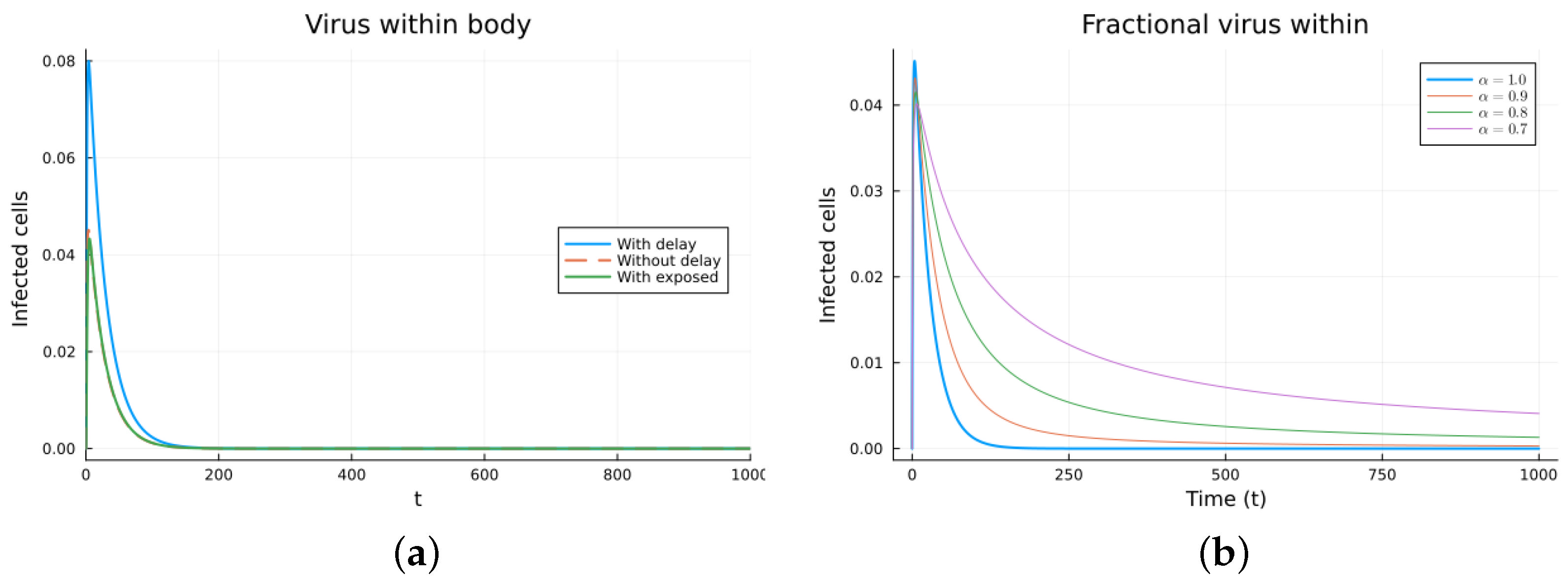
Finally, we consider a more complicated model in which the populations can interact in several ways, and there are two terms of the equations for the susceptible and infected cells that have a delay. There is also a second delay. The values of the parameters used are $\mathsf{\Lambda }$ = 5 × 10⁵ (cells/mL), ${\mu }_x$ = 0.003 (1/day), $\beta$ = 4 × 10⁻¹⁰ (mL/(cells day)), ${\mu }_y$ = 0.043 (1/day), ${\mu }_v$ = 0.7 (1/day), B = 5.58, ${\beta }_{xy}=\beta /3$ (mL/(cells day)), ${\mu }_E=0.5$ (1/day), ${\alpha }_1$ = 2.2 × 10⁻⁷ (1/day), ${\beta }_{E}y$ = 0.6 × 10⁻³ (mL/(cells day)), ${\beta }_{yE}={\beta }_{Ey}$ (mL/(cells day)), ${\beta }_{Ev}$ = 4 × 10⁻¹⁰ (mL/(cells day)), ${\beta }_{vE}$ = ${\beta }_{Ev}$ (mL/(cells day)), s = 30 (cells/(mL day)), ${\tau }_1$ = 1 (day), and ${\tau }_2$ = 24 (day). These parameters are based on those in [55,56] for liver infection by the hepatitis B virus. The initial conditions are $x\left(0\right)=\mathsf{\Lambda }/{\mu }_x,y\left(0\right)=0,v\left(0\right)=0.33,$ and $E\left(0\right)=s/{\mu }_E$. Figure 10, Figure 11, Figure 12 and Figure 13 show the simulations for the above-mentioned values of the parameters. The plots on the left of the figures correspond to the simulations using (22), (23), and (25). For the values of the parameters given above, the solutions tend to a chronic equilibrium state. The DFE is asymptotically unstable for the integer-order models, as was also shown in [66]. The plots on the right correspond to the simulations using (24) for different values of the order of the derivative $\alpha$. As expected, for the number of infected cells, for the fractional model, the rate of increase of the solutions increases as $\alpha$ increases toward 1. The optimal value of $\alpha$ is between 0.9 and 1. Since the solutions increased very slowly, the plots were truncated to clearly show the differences for a short time. Another simulation was conducted with ${\beta }_{xy}=0$, resulting in no transmission from cell to cell. In this case, the DFE is asymptotically stable, as illustrated in Figure 14.

4. Discussion

Many populations depend on their values in the past. The number of births depends on the population the maturation time ago. The number of newly infected depends on the number of contacts between an infected and a susceptible the infection time ago. Also, the immune system takes a certain time to react and start fighting an infection. Mathematical models for processes involving values in the past should incorporate this dependence and, therefore, produce solutions that are more realistic. Mathematical models are simplifications of reality. This can be due to keeping the model tractable or to the lack of information and data. ODE-based models assume that the population is homogeneously distributed and so avoid having spatial dependence. Usually, infection rates are assumed to be constant but they can vary with time, temperature, and the individual. There may be saturation effects not modeled by mass-action kinetics. Recovered individuals turning into susceptibles may retain some immunity and may infect others. Processes that take time should be modeled taking into account that time. As shown in Section 2, there are different ways of introducing delays into an ODE model, but they need to be introduced in a consistent manner. For example, model (19) does not conserve the total population and, therefore, should not be used. The maturation time is not a single time but has some variation. The same is true for the infection time. But usually, these variations are small, and using a single value is a good approximation. But if they are not, then a distributed delay model will be better. Also, there is the effect of population values on the history interval, $[t_0-\tau ,t_0]$, where $t_0$ is the initial time. But for epidemic or infection models, the values of the populations in those intervals can be assumed to correspond to the DFE, which is a reasonable assumption. There are many papers dealing with comparisons between a variety of epidemic models with delays and real data for diseases like dengue or COVID-19. A few examples can be found in [67,68,69,70]. Most show that the fit is good but do not compare their results with those of other methods. An exception is [70], where the results from a DDE model were compared with those from an ODE model.

A second way to introduce dependence on the past is to replace the time derivative with a fractional one. From the definition, for example, of the Caputo derivative at time t, it is a weighted average of the time derivatives at times from 0 to the current time t. As shown in Section 2, FDEs do not come from discrete-time conservation models by taking the limit as the time increment goes to zero. In models where the dependence on past times comes from the delay in a given process, the FDEs do not have a form similar to constant or distributed delay models. Furthermore, the effect of past times starts with the initial time of modeling, as opposed to models formulated using DDEs, where the influence extends over times $t\in [t_0-\tau ,t_0]$, with $\tau$ representing the delay. FDEs introduce memory, but there lacks a justification for the specific form of this memory. For epidemic models, it is true that susceptibles may remember previous infections, potentially leading to a different infection process. But this does not justify the form of the memory in the FDE. It is also true that many epidemic models based on FDEs fit data better than models based on ODEs, but this may be due to the additional parameter $\alpha$. If there are susceptibles who previously had the infection and thus may react differently to a new infection due to their memory of the previous infection, an alternative is to add a new susceptible compartment. This can also be done for infectives and those who have recovered from previous infections. The main arguments for using FDEs in epidemic models are that they include memory and that they fit data better than models based on ODEs. This is true, but there is no justification that the memory that the FDEs provide has anything to do with any biological, physical, or chemical process with dependence on the past. Also, the value of the fractional order (or orders) is chosen to better fit the data. Mechanistic models should give a modeling reason or hypothesis on how to choose it. Statistical models, like linear regression, will find the values of the involved parameters to better fit a data set. But mechanistic models should do more than provide computational data that fit experimental data. Recently, there has been an awareness that fractional differential equations should also include delays to better model processes that have delays. This allows the fractional derivative to provide an additional memory effect. Some references supporting this notion are [71,72,73].

A third common way to introduce that processes take time, thus introducing dependence on the past, is to add new populations, immature populations for birth processes, or exposed populations or cells to epidemic or infection models. This approach has the advantage of being based on ODEs, and, for example, the next-generation matrix method can be used to determine if there will be an epidemic. Also, it does not require initial values for an interval prior to the initial value of t. But, just as a Malthus death model $\frac{dN}{dt}=-\mu N$ with $\mu >0$ can have individuals living for very long times, some exposed individuals may stay in the compartment for a long time. Of course, this can happen with a very small probability.

All the example models used have a dependence on past values based on the assumption that the dependence is due to the time it takes processes like infection or maturation to happen. Delay models, as well as exposed or immature models, explicitly include this dependence. Fractional differential equation models have a dependence on past values, but this dependence has a different form that is independent of the actual value of the delay or delays. But fractional differential equation models offer the flexibility of more parameters, specifically the fractional orders of the derivatives. By choosing these orders adequately, these models can produce similar results to models that explicitly include the delays.

In conclusion, the terms added to an ODE model to take into account dependence on past values need justification. The justification should be more than just saying there is memory or achieving a better fit. The processes in mechanistic mathematical models need to be based on realistic assumptions. For processes depending on past values due to a delay, DDEs are good choices since there is flexibility in choosing the form of the delay, whether constant or distributed. But models based on adding more populations and still relying on ODEs are simpler to analyze. When using fractional derivatives, modeling assumptions should also be clearly stated.

Future work will include models with stochastic delays, models with partial immunity, and comparisons of the predicted results with real data.

References

- Kuang, Y. Delay Differential Equations: With Applications in Population Dynamics; Academic Press: Cambridge, MA, USA, 1993. [Google Scholar]
- Bellen, A.; Zennaro, M. Numerical Methods for Delay Differential Equations; Oxford University Press: Oxford, UK, 2013. [Google Scholar]
- Wang, W. Modeling of Epidemics with Delays and Spatial Heterogeneity. In Dynamical Modeling and Analysis of Epidemics; World Scientific: Singapore, 2009; pp. 201–272. [Google Scholar]
- Cooke, K.L. Stability analysis for a vector disease model. Rocky Mt. J. Math. 1979, 9, 31–42. [Google Scholar] [CrossRef]
- Ruan, S. Delay differential equations in single species dynamics. In Delay Differential Equations and Applications; Springer: Dordrecht, The Netherlands, 2006; pp. 477–517. [Google Scholar]
- McCluskey, C.C. Complete global stability for an SIR epidemic model with delay—Distributed or discrete. Nonlinear Anal. Real World Appl. 2010, 11, 55–59. [Google Scholar] [CrossRef]
- Avila-Vales, E.; Pérez, Á.G. Dynamics of a time-delayed SIR epidemic model with logistic growth and saturated treatment. Chaos Solitons Fractals 2019, 127, 55–69. [Google Scholar] [CrossRef]
- Kumar, A.; Goel, K.; Nilam. A deterministic time-delayed SIR epidemic model: Mathematical modeling and analysis. Theory Biosci. 2020, 139, 67–76. [Google Scholar] [CrossRef] [PubMed]
- Podlubny, I. Fractional Differential Equations: An Introduction to Fractional Derivatives, Fractional Differential Equations, to Methods of Their Solution and Some of Their Applications; Elsevier: Amsterdam, The Netherlands, 1998. [Google Scholar]
- Kilbas, A.A.; Srivastava, H.M.; Trujillo, J.J. Theory and Applications of Fractional Differential Equations; Elsevier: Amsterdam, The Netherlands, 2006; Volume 204. [Google Scholar]
- Li, C.; Zhang, F. A survey on the stability of fractional differential equations: Dedicated to Prof. YS Chen on the Occasion of his 80th Birthday. Eur. Phys. J. Spec. Top. 2011, 193, 27–47. [Google Scholar] [CrossRef]
- Jin, B. Fractional Differential Equations; Springer: Cham, Switzerland, 2021. [Google Scholar]
- González-Parra, G.; Arenas, A.J.; Chen-Charpentier, B.M. A fractional order epidemic model for the simulation of outbreaks of influenza A (H1N1). Math. Methods Appl. Sci. 2014, 37, 2218–2226. [Google Scholar] [CrossRef]
- Area, I.; Batarfi, H.; Losada, J.; Nieto, J.J.; Shammakh, W.; Torres, Á. On a fractional order Ebola epidemic model. Adv. Differ. Equ. 2015, 2015, 278. [Google Scholar] [CrossRef]
- Hamdan, N.; Kilicman, A. A fractional order SIR epidemic model for dengue transmission. Chaos Solitons Fractals 2018, 114, 55–62. [Google Scholar] [CrossRef]
- Chatterjee, A.N.; Ahmad, B. A fractional-order differential equation model of COVID-19 infection of epithelial cells. Chaos Solitons Fractals 2021, 147, 110952. [Google Scholar] [CrossRef]
- Chen, Y.; Liu, F.; Yu, Q.; Li, T. Review of fractional epidemic models. Appl. Math. Model. 2021, 97, 281–307. [Google Scholar] [CrossRef]
- Petrás, I. Fractional Derivatives, Fractional Integrals, and Fractional Differential Equations in Matlab; IntechOpen: London, UK, 2011. [Google Scholar]
- Scherer, R.; Kalla, S.L.; Tang, Y.; Huang, J. The Grünwald–Letnikov method for fractional differential equations. Comput. Math. Appl. 2011, 62, 902–917. [Google Scholar] [CrossRef]
- Li, Z.; Liu, L.; Dehghan, S.; Chen, Y.; Xue, D. A review and evaluation of numerical tools for fractional calculus and fractional order controls. Int. J. Control 2017, 90, 1165–1181. [Google Scholar] [CrossRef]
- Garrappa, R. Numerical solution of fractional differential equations: A survey and a software tutorial. Mathematics 2018, 6, 16. [Google Scholar] [CrossRef]
- Li, T.; Wang, Y.; Liu, F.; Turner, I. Novel parameter estimation techniques for a multi-term fractional dynamical epidemic model of dengue fever. Numer. Algorithms 2019, 82, 1467–1495. [Google Scholar] [CrossRef]
- Das, M.; Samanta, G.; De la Sen, M. A Fractional Ordered COVID-19 Model Incorporating Comorbidity and Vaccination. Mathematics 2021, 9, 2806. [Google Scholar] [CrossRef]
- Atici, F.; Eloe, P. Initial value problems in discrete fractional calculus. Proc. Am. Math. Soc. 2009, 137, 981–989. [Google Scholar] [CrossRef]
- Cheng, J.F.; Chu, Y.M. Fractional difference equations with real variable. Abstr. Appl. Anal. 2012, 2012, 918529. [Google Scholar] [CrossRef]
- Ferreira, R.A. Discrete Fractional Calculus and Fractional Difference Equations; Springer: Cham, Switzerland, 2022. [Google Scholar]
- Esteva, L.; Yang, H.M. Mathematical model to assess the control of Aedes aegypti mosquitoes by the sterile insect technique. Math. Biosci. 2005, 198, 132–147. [Google Scholar] [CrossRef]
- Anguelov, R.; Dumont, Y.; Lubuma, J. Mathematical modeling of sterile insect technology for control of anopheles mosquito. Comput. Math. Appl. 2012, 64, 374–389. [Google Scholar] [CrossRef]
- Li, M.Y.; Muldowney, J.S. Global stability for the SEIR model in epidemiology. Math. Biosci. 1995, 125, 155–164. [Google Scholar] [CrossRef]
- Jeger, M.; Madden, L.; Van Den Bosch, F. Plant virus epidemiology: Applications and prospects for mathematical modeling and analysis to improve understanding and disease control. Plant Dis. 2018, 102, 837–854. [Google Scholar] [CrossRef]
- He, S.; Peng, Y.; Sun, K. SEIR modeling of the COVID-19 and its dynamics. Nonlinear Dyn. 2020, 101, 1667–1680. [Google Scholar] [CrossRef]
- Agaba, G.O.; Soomiyol, M.C. Analysing the spread of COVID-19 using delay epidemic model with awareness. IOSR J. Math. 2020, 16, 52–59. [Google Scholar]
- Babasola, O.; Kayode, O.; Peter, O.J.; Onwuegbuche, F.C.; Oguntolu, F.A. Time-delayed modelling of the COVID-19 dynamics with a convex incidence rate. Inform. Med. Unlocked 2022, 35, 101124. [Google Scholar] [CrossRef]
- Sepulveda, G.; Arenas, A.J.; González-Parra, G. Mathematical Modeling of COVID-19 dynamics under two vaccination doses and delay effects. Mathematics 2023, 11, 369. [Google Scholar] [CrossRef]
- Zhang, J. Pandemic Mathematical Models, Epidemiology, and Virus Origins. In Optimization-Based Molecular Dynamics Studies of SARS-CoV-2 Molecular Structures: Research on COVID-19; Springer: Cham, Switzerland, 2023; pp. 897–908. [Google Scholar]
- Dickson, S.; Padmasekaran, S.; Kumar, P. Fractional order mathematical model for B. 1.1. 529 SARS-Cov-2 Omicron variant with quarantine and vaccination. Int. J. Dyn. Control 2023, 11, 2215–2231. [Google Scholar] [CrossRef]
- Allen, L. An Introduction to Mathematical Biology; Pearson-Prentice Hall: Hoboken, NJ, USA, 2007. [Google Scholar]
- Edelstein-Keshet, L. Mathematical Models in Biology; SIAM: Philadelphia, PA, USA, 2005. [Google Scholar]
- Castillo-Chavez, C.; Yakubu, A.A. Discrete-time SIS models with simple and complex population dynamics. IMA Vol. Math. Its Appl. 2002, 125, 153–164. [Google Scholar]
- Brauer, F.; Feng, Z.; Castillo-Chavez, C. Discrete epidemic models. Math. Biosci. Eng. 2009, 7, 1–15. [Google Scholar]
- Cooke, K.L.; Yorke, J.A. Some equations modelling growth processes and gonorrhea epidemics. Math. Biosci. 1973, 16, 75–101. [Google Scholar] [CrossRef]
- Khan, Q.J.A.; Krishnan, E.V. An Epidemic Model with a Time Delay in Transmission. Appl. Math. 2003, 48, 193–203. [Google Scholar] [CrossRef]
- Jackson, M.; Chen-Charpentier, B.M. Modeling plant virus propagation with delays. J. Comput. Appl. Math. 2017, 309, 611–621. [Google Scholar] [CrossRef]
- Liu, L. A delayed SIR model with general nonlinear incidence rate. Adv. Differ. Equ. 2015, 2015, 329. [Google Scholar] [CrossRef]
- Hethcote, H.W. The Mathematics of Infectious Diseases. SIAM Rev. 2000, 42, 599–653. [Google Scholar] [CrossRef]
- Al-Sulami, H.; El-Shahed, M.; Nieto, J.J.; Shammakh, W. On fractional order dengue epidemic model. Math. Probl. Eng. 2014, 2014, 456537. [Google Scholar] [CrossRef]
- Sardar, T.; Rana, S.; Bhattacharya, S.; Al-Khaled, K.; Chattopadhyay, J. A generic model for a single strain mosquito-transmitted disease with memory on the host and the vector. Math. Biosci. 2015, 263, 18–36. [Google Scholar] [CrossRef]
- Legg, J.P.; Kumar, P.L.; Makeshkumar, T.; Tripathi, L.; Ferguson, M.; Kanju, E.; Ntawuruhunga, P.; Cuellar, W. Cassava virus diseases: Biology, epidemiology, and management. In Advances in Virus Research; Elsevier: Amsterdam, The Netherlands, 2015; Volume 91, pp. 85–142. [Google Scholar]
- Gyamera, E.A.; Domfeh, O.; Ameyaw, G.A. Cacao Swollen Shoot Viruses in Ghana. Plant Dis. 2023, 107, 1261–1278. [Google Scholar] [CrossRef] [PubMed]
- Shi, R.; Zhao, H.; Tang, S. Global dynamic analysis of a vector-borne plant disease model. Adv. Differ. Equ. 2014, 2014, 59. [Google Scholar] [CrossRef]
- Erneux, T. Applied Delay Differential Equations; Springer Science & Business Media: New York, NY, USA, 2009; Volume 3. [Google Scholar]
- Anwar, N.; Naz, S.; Shoaib, M. Reliable numerical treatment with Adams and BDF methods for plant virus propagation model by vector with impact of time lag and density. Front. Appl. Math. Stat. 2022, 8, 1001392. [Google Scholar] [CrossRef]
- Diekmann, O.; Heesterbeek, J.; Roberts, M.G. The construction of next-generation matrices for compartmental epidemic models. J. R. Soc. Interface 2010, 7, 873–885. [Google Scholar] [CrossRef] [PubMed]
- Van den Driessche, P. Reproduction numbers of infectious disease models. Infect. Dis. Model. 2017, 2, 288–303. [Google Scholar] [CrossRef] [PubMed]
- Ciupe, S.M.; Ribeiro, R.M.; Nelson, P.W.; Dusheiko, G.; Perelson, A.S. The role of cells refractory to productive infection in acute hepatitis B viral dynamics. Proc. Natl. Acad. Sci. USA 2007, 104, 5050–5055. [Google Scholar] [CrossRef]
- Kim, H.Y.; Kwon, H.D.; Jang, T.S.; Lim, J.; Lee, H.S. Mathematical modeling of triphasic viral dynamics in patients with HBeAg-positive chronic hepatitis B showing response to 24-week clevudine therapy. PLoS ONE 2012, 7, e50377. [Google Scholar] [CrossRef]
- Pourbashash, H.; Pilyugin, S.S.; De Leenheer, P.; McCluskey, C. Global analysis of within host virus models with cell-to-cell viral transmission. Discret. Contin. Dyn. Syst. Ser. B 2014, 19, 3341–3357. [Google Scholar] [CrossRef]
- Zhang, S.; Li, F.; Xu, X. Dynamics and control strategy for a delayed viral infection model. J. Biol. Dyn. 2022, 16, 44–63. [Google Scholar] [CrossRef]
- Rihan, F.A. Delay Differential Equations and Applications to Biology; Springer: Singapore, 2021. [Google Scholar]
- Wolfram Research, Inc. Mathematica, version 13.2; Wolfram: Champaign, IL, USA, 2022. [Google Scholar]
- Rackauckas, C.; Nie, Q. DifferentialEquations.jl—A Performant and Feature-Rich Ecosystem for Solving Differential Equations in Julia. J. Open Res. Softw. 2017, 5, 15. Available online: https://app.dimensions.aion2019/05/05 (accessed on 3 March 2024). [CrossRef]
- Widmann, D.; Rackauckas, C. DelayDiffEq: Generating Delay Differential Equation Solvers via Recursive Embedding of Ordinary Differential Equation Solvers. arXiv 2022, arXiv:2208.12879. [Google Scholar]
- Khalighi, M.; Benedetti, G.; Lahti, L. Fdesolver: A julia package for solving fractional differential equations. arXiv 2022, arXiv:2212.12550. [Google Scholar]
- Kermack, W.O.; McKendrick, A.G. Contributions to the mathematical theory of epidemics–I. 1927. Bull. Math. Biol. 1991, 53, 33–55. [Google Scholar] [PubMed]
- Hattaf, K. On the Stability and Numerical Scheme of Fractional Differential Equations with Application to Biology. Computation 2022, 10, 97. [Google Scholar] [CrossRef]
- Chen-Charpentier, B. A Model of Hepatitis B Viral Dynamics with Delays. AppliedMath 2024, 4, 182–196. [Google Scholar] [CrossRef]
- Wu, C.; Wong, P.J. Dengue transmission: Mathematical model with discrete time delays and estimation of the reproduction number. J. Biol. Dyn. 2019, 13, 1–25. [Google Scholar] [CrossRef] [PubMed]
- Dell’Anna, L. Solvable delay model for epidemic spreading: The case of Covid-19 in Italy. Sci. Rep. 2020, 10, 15763. [Google Scholar] [CrossRef] [PubMed]
- Shayak, B.; Sharma, M.M.; Rand, R.H.; Singh, A.; Misra, A. A Delay differential equation model for the spread of COVID-19. Int. J. Eng. Res. Appl. 2020, 10, 1–13. [Google Scholar]
- Saade, M.; Ghosh, S.; Banerjee, M.; Volpert, V. An epidemic model with time delays determined by the infectivity and disease durations. Math. Biosci. Eng. 2023, 20, 12864–12888. [Google Scholar] [CrossRef] [PubMed]
- Rihan, F.; Al-Mdallal, Q.; AlSakaji, H.; Hashish, A. A fractional-order epidemic model with time-delay and nonlinear incidence rate. Chaos Solitons Fractals 2019, 126, 97–105. [Google Scholar] [CrossRef]
- Singh, H. Numerical simulation for fractional delay differential equations. Int. J. Dyn. Control 2021, 9, 463–474. [Google Scholar] [CrossRef]
- Sun, D.; Liu, J.; Su, X.; Pei, G. Fractional differential equation modeling of the HBV infection with time delay and logistic proliferation. Front. Public Health 2022, 10, 1036901. [Google Scholar] [CrossRef]
Figure 1.
Flow diagram for the sequence of models used, from simplest to most complex. ODE is the ordinary differential equations model, DDE is the delay differential equations model, EXP is the model with immature or exposed populations, and FRAC is the fractional differential equations model. E indicates that the model has an exact solution, S indicates the local asymptotic stability of the steady states for the Malthus and logistic models, and of the disease-free equilibrium for the infection models.
Figure 2.
Malthus models. (a) ODE, DDE, and immature population models. The legend “Both” refers to the sum of the mature and immature populations for model (5). (b) Fractional models for several values of .
Figure 3.
Logistic models. (a) ODE, DDE, and immature population models. The legend “Both” refers to the sum of the mature and the young or immature populations for model (8). (b) Fractional models for several values of .
Figure 4.
SIRS models, susceptibles. (a) ODE, DDE, and SEIRS models. (b) Fractional models for several values of .
Figure 5.
SIRS models, infectives. (a) ODE, DDE, and SEIRS models. (b) Fractional models for several values of .
Figure 6.
Plant vector virus models, susceptible plants. (a) ODE, DDE, and exposed population models. (b) Fractional models for several values of .
Figure 7.
Plant vector virus models, infected plants. (a) ODE, DDE, and exposed population models. (b) Fractional models for several values of .
Figure 8.
Plant vector virus models, susceptible vectors. (a) ODE, DDE, and exposed population models. (b) Fractional models for several values of .
Figure 9.
Plant vector virus models, infected vectors. (a) ODE, DDE, and exposed population models. (b) Fractional models for several values of .
Figure 10.
Virus within-host models, susceptible cells. (a) ODE, DDE, and exposed population models. (b) Fractional models for several values of .
Figure 11.
Virus within-host models, infected cells. (a) ODE, DDE, and exposed population models. (b) Fractional models for several values of .
Figure 12.
Virus within-host models, virus particles. (a) ODE, DDE, and exposed population models. (b) Fractional models for several values of .
Figure 13.
Virus within-host models, effector cells. (a) ODE, DDE, and exposed population models. (b) Fractional models for several values of .
Figure 14.
Virus within-host models, infected cells, for . (a) ODE, DDE, and exposed population models. (b) Fractional models for several values of .
Disclaimer/Publisher’s Note: The statements, opinions and data contained in all publications are solely those of the individual author(s) and contributor(s) and not of MDPI and/or the editor(s). MDPI and/or the editor(s) disclaim responsibility for any injury to people or property resulting from any ideas, methods, instructions or products referred to in the content. |
© 2024 by the author. Licensee MDPI, Basel, Switzerland. This article is an open access article distributed under the terms and conditions of the Creative Commons Attribution (CC BY) license (https://creativecommons.org/licenses/by/4.0/).
Share and Cite
MDPI and ACS Style
Chen-Charpentier, B. On Population Models with Delays and Dependence on Past Values. Axioms 2024, 13, 206. https://doi.org/10.3390/axioms13030206
AMA Style
Chen-Charpentier B. On Population Models with Delays and Dependence on Past Values. Axioms. 2024; 13(3):206. https://doi.org/10.3390/axioms13030206
Chicago/Turabian StyleChen-Charpentier, Benito. 2024. "On Population Models with Delays and Dependence on Past Values" Axioms 13, no. 3: 206. https://doi.org/10.3390/axioms13030206
Note that from the first issue of 2016, this journal uses article numbers instead of page numbers. See further details here.