Article

Simpson’s Variational Integrator for Systems with Quadratic Lagrangians

by
Juan Antonio Rojas-Quintero
1,2,*,
François Dubois
3,4 and
José Guadalupe Cabrera-Díaz
5
1
CONAHCYT, Tecnológico Nacional de México, I. T. Ensenada, Ensenada 22780, B.C., Mexico
2
IMT Atlantique, LS2N, UMR CNRS 6004, 44307 Nantes, France
3
Université Paris-Saclay, Laboratoire de Mathématiques d’Orsay, 91400 Orsay, France
4
Conservatoire National des Arts et Métiers, Structural Mechanics and Coupled Systems Laboratory, 75141 Paris, France
5
Tecnológico Nacional de México, I. T. Ensenada, Ensenada 22780, B.C., Mexico
*
Author to whom correspondence should be addressed.
Axioms 2024, 13(4), 255; https://doi.org/10.3390/axioms13040255
Submission received: 5 February 2024 / Revised: 5 April 2024 / Accepted: 9 April 2024 / Published: 11 April 2024
(This article belongs to the Special Issue Advances in Dynamical Systems and Control)

Abstract

:
This contribution proposes a variational symplectic integrator aimed at linear systems issued from the least action principle. An internal quadratic finite-element interpolation of the state is performed at each time step. Then, the action is approximated by Simpson’s quadrature formula. The implemented scheme is implicit, symplectic, and conditionally stable. It is applied to the time integration of systems with quadratic Lagrangians. The example of the linearized double pendulum is treated. Our method is compared with Newmark’s variational integrator. The exact solution of the linearized double pendulum example is used for benchmarking. Simulation results illustrate the precision and convergence of the proposed integrator.

1. Introduction

Simpson’s quadrature is the name that is generally given to a numerical approximation of definite integrals that is exact for polynomials up to the third degree:
0 1 ψ ( θ ) θ 1 6 ψ ( 0 ) + 4 ψ 1 2 + ψ ( 1 ) .
It is well known that this rule was found by Bonaventura Cavalieri (1598–1647), known to James Gregory (1638–1675) [1], and even used by Johannes Kepler (1571–1630) to approximate the volume of barrels [2]. However, Thomas Simpson (1710–1761) is usually credited for this rule. As such, Formula (1) is also widely known as Simpson’s 1 3 rule. It corresponds to a special case of Newton–Cotes’s formula [1] and coincides with the classical fourth-order Runge–Kutta method [1,3].
Generally, numerical methods involving Simpson’s quadrature estimate a definite integral by using quadratic polynomials to approximate the integrand on a sequence of intervals. This general idea is at the foundation of numerous methods that can be applied to solve engineering problems such as the low-thrust orbit transfer problem [4] or the gait optimization of a bipedal walking robot [5]. Recently, much attention has been brought to fractional calculus, for which solvers based on Simpson’s quadrature (adapted to the fractional form) have been developed [6]. Some applications involve solving initial-value problems of fractional differential systems [7] or the solution of fractional equations affected by noisy signals [8]. Another recent application of Simpson’s quadrature involves the solution of partial integro-differential equations [9].
Our contribution is aimed at solving differential equations characterizing the motions of mechanical systems. It is well known that the motions of a mechanical system are the extremals of the variational principle of least action [10]. This principle is one of the most general laws of theoretical physics and is foundational for characterizing a system’s evolution in the form of differential equations. It is valid across disciplines such as classical and quantum mechanics, cosmology, electromagnetism, optics, and relativity [10,11,12,13,14]. As such, this variational principle is closely involved in the development of the finite-element method [15], which is used for the space and time integration of differential equations [16].
Numerical schemes for dynamical systems issued from the principle of least action are typically referred to as variational [17,18,19,20]. The general idea resides in performing a discretization at the least action principle level. As a result, the evolution equations deriving from this discretized principle characterize the system evolution, but are also a numerical scheme. It is well known that such numerical methods are endowed with interesting characteristics; one characteristic is the property of being symplectic [18,19,20,21]. One remarkable example of such methods is Newmark’s integrator [17,19], which is very popular for solving problems in the dynamics of structures [22,23] and has recently been geometrized to solve the motion equations of sliding rods [24] and soft robots [25].
A symplectic scheme based on Simpson’s rule has been proposed by the authors in [26], for the linear and scalar case of the harmonic oscillator. The scheme uses a quadratic finite-element interpolation. The method was adapted to the monodimensional non-linear pendulum system in [27]. In this work, Simpson’s symplectic scheme is further studied as an alternative to Newmark’s method. It is generalized to the case of multiple-degrees of freedom systems characterized by quadratic Lagrangians. The obtained results confirm the convergence rate previously observed in [26]. The new stability condition on the step size is revealed to be similar to the one previously obtained in [26]. A simplecticity analysis that applies to the multi-degree of freedom case, along with the expression of a related conserved quadratic form, is provided in this contribution.
We begin our study by detailing Newmark’s classical scheme, deriving it from variational principles in Section 2. Then, Simpson’s alternative scheme is detailed and derived from variational principles in Section 3. Section 4 analyzes the symplectic property of Simpson’s scheme. A proof that applies to both Newmark’s and Simpson’s schemes is provided. To compare both methods in a case study, a two-degree of freedom system is presented. Therefore, the exact solution to the linearized double pendulum is provided in Section 5. This exact solution serves for benchmarking purposes in our comparisons. Section 6 presents and comments on the obtained numerical results. Simpson’s scheme’s convergence is revealed to be of the fourth order. The manuscript ends with a brief discussion and concluding remarks in Section 7.

2. Newmark’s Scheme

2.1. Discrete Action

Let us derive the classical, symplectic variational integrator based on Newmark’s scheme [17,19,22,23]. The continuous action is defined as
S c = 0 T L d q ( t ) d t , q ( t ) t
where L is the system Lagrangian. We focus on dynamical systems for which the Lagrangian can be expressed quadratically as
L = 1 2 q ˙ T M q ˙ 1 2 q T K q ,
where M and K are symmetric, positive-definite n-dimensional matrices with constant coefficients; q R n .
We can discretize Equation (2) by splitting the simulation interval [ 0 , T ] into N elements using a time step h = T N . An approximation q j of q ( t j ) is calculated at each instance t j = j h . The following action S d represents the discrete version of Equation (2):
S d = j = 1 N 1 L d q j , q j + 1 ,
where L d q , q r is the discrete form of the Lagrangian (3). Subscripts and r stand for “left” and “right” values, respectively. Let us consider a centered finite-difference approximation:
d q d t q r q h ,
and a midpoint quadrature:
0 h φ ( q ( t ) ) t h φ q + q r 2 .
The discrete Lagrangian becomes
L d ( q , q r ) = h 2 q r q h T M q r q h h 2 q + q r 2 T K q + q r 2 .

2.2. Discrete Euler–Lagrange Equations

The discrete action (4) being a sum, only two terms contain the variables q j :
S d = + L d q j 1 , q j + L d q j , q j + 1 + .
So, when the discrete action is stationary ( δ S d = 0 for arbitrary variations δ q j of the states q j ), only two terms remain. Necessarily,
L d q r q j 1 , q j + L d q q j , q j + 1 = 0 .
The generalized momenta p j R n are defined, on the right, as
p j = L d q r q , q r .
Therefore, the first term of Equation (5) is identified as p j , so applying Equation (6) in Equation (5) leads to
p j = L d q q j , q j + 1 = M q j + 1 q j h + h 2 K q j + q j + 1 2 .
Then, p j + 1 is constructed following Equation (6):
p j + 1 = M q j + 1 q j h h 2 K q j + q j + 1 2 .
Using Equations (7) and (8), it can be established that
p j + 1 p j h = K q j + q j + 1 2 ; p j + p j + 1 2 = M q j + 1 q j h .
Equations (9) are consistent with d p d t = K q and p = M d q d t , respectively.

2.3. Newmark’s Scheme

System (9) can then be arranged in linear form as
A n η j + 1 = B n η j ,
where η R 2 n , η = ( p , q ) T and
A n = I n X n I n Y n ; B n = I n X n I n Y n ; X n = 2 h M ; Y n = h 2 K ;
I n is the n-dimensional identity matrix.
Newmark’s symplectic scheme is obtained by matrix inversion of Equation (10). We can establish that
η j + 1 = Φ n η j , Φ n = A n 1 B ,
where matrices A and B are defined in Equation (11) above. It has been observed that this particular variant of Newmark’s method is unconditionally stable and second-order convergent [19].

3. Simpson’s Scheme

Newmark’s scheme, presented in Section 2, uses a midpoint quadrature for the numerical integration of a regular function. This quadrature is exact only for polynomials up to the first degree. A better precision is obtained with Simpson’s quadrature (1), which is exact for polynomials up to the third degree. Notice how Formula (1) introduces a midpoint. This midpoint will be regarded as an additional degree of freedom in our proposed integrator.
Let us now derive a symplectic scheme based on this integration rule. As with Newmark’s scheme, the continuous action is defined by Equation (2) and the Lagrangian has the structure of Equation (3).

3.1. Quadratic Finite-Element Interpolation

An internal interpolation can be performed at each time step, for t [ 0 , h ] , using quadratic finite elements [16,28]. We use the following compact basis functions for 0 θ 1 :
φ 0 ( θ ) = ( 1 θ ) ( 1 2 θ ) , φ 1 2 ( θ ) = 4 θ ( 1 θ ) , φ 1 ( θ ) = θ ( 2 θ 1 ) .
At t = h θ , the states q ( t ) P 2 are approximated with the above basis functions as
q ( t ) = q φ 0 ( θ ) + q m φ 1 2 ( θ ) + q r φ 1 ( θ ) .
Note that q ( 0 ) = q , q h 2 = q m and q ( h ) = q r ; here, subscript m stands for “middle”.
This means that the finite-elements (13) are well adapted to the internal degree of freedom at h 2 . Then, by time differentiation,
d q d t = 1 h q d φ 0 d θ + q m d φ 1 2 d θ + q r d φ 1 d θ = 1 h q ( 4 θ 3 ) + 4 q m ( 1 2 θ ) + q r ( 4 θ 1 ) = g ( 1 θ ) + g r θ
where derivatives g , g r R n are given by Gear’s scheme [29]. Gear’s scheme is used as the differentiation approximation for q ( t ) P 2 as
g = d q d t ( 0 ) = 1 h ( 3 q + 4 q m q r ) , g m = d q d t h 2 = g + g r 2 = q r q h , g r = d q d t ( h ) = 1 h q 4 q m + 3 q r ,
where g m R n . The above confirms that a first-order centered finite difference is recovered by g m , which is the derivative at the middle of the discretization interval.
The interpolation is used within an interval of length h by splitting the range [ 0 , T ] into N pieces, giving a fixed step size of h = T N . At each discrete time instance t j = j h , we have
q j q ( t j ) , 0 j N ; q j + 1 2 q t j + h 2 , 0 j N 1 .
Taking Equation (14), q ( t ) is a quadratic polynomial vector function within the interval [ t j , t j + 1 ] with
t = t j + θ h , q = q j , q m = q j + 1 2 , q r = q j + 1 .

3.2. Discrete Lagrangian

Let us recall that the continuous action is defined by Equation (2) and that the Lagrangian is defined by Equation (3). In the present case, the discrete action sum Σ d for a motion t q ( t ) between the initial time and a given final time T > 0 is discretized with N regular intervals as
Σ d = j = 1 N 1 L h q j , q j + 1 2 , q j + 1 ,
where L h q , q m , q r is the discrete form
L h q , q m , q r 0 h L t ,
of the Lagrangian (3). Using Simpson’s rule (1), the polynomial approximation (14) of the states, and derivatives (15), the discrete Lagrangian of a linear system is expressed as
L h ( q , q m , q r ) = h 2 1 6 g T M g + 2 3 g m T M g m + 1 6 g r T M g r h 2 1 6 q T K q + 2 3 q m T K q m + 1 6 q r T K q r .

3.3. Discrete Euler–Lagrange Equations

Recall that Simpson’s rule introduces an internal degree of freedom in the middle of the interpolation interval. The discrete action (16) is a sum where only two terms contain the variables q j and q j + 1 2 :
Σ d = + L h q j 1 , q j 1 2 , q j + L h q j , q j + 1 2 , q j + 1 +
Maupertuis’s stationary action principle [10] implies that δ Σ d = 0 for an arbitrary variation of the internal degree of freedom δ q j + 1 2 [ t j , t j + 1 ] . Considering Gear’s scheme (15), we have
g i q m k = 4 h , g m i q m k = 0 , g r i q m k = 4 h , i = k , 0 otherwise ,
where g i is the i-th component of g and q k is the k-th component of q .
When δ Σ d = 0 , L h q m q j , q j + 1 2 , q j + 1 = 0 by necessity. This conforms to the discrete Euler–Lagrange equations at the middle of the interpolation interval:
4 3 h M g j 4 3 h M g j + 1 4 3 K q j + 1 2 = 0 .
However, g j g j + 1 = 1 h 4 q j + 8 q j + 1 2 4 q j + 1 , so Equation (17) becomes
M 4 q j 2 q j + 1 2 + q j + 1 h 2 + K q j + 1 2 = 0 .
This last equation is consistent with M d 2 q d t 2 + K q = 0 .
Additionally, for an arbitrary variation δ q j , the Euler–Lagrange equations are given by the necessary condition that
L d q r q j 1 , q j 1 2 , q j + L d q q j , q j + 1 2 , q j + 1 = 0 .
The generalized momenta p j are defined, on the right, as
p j = L d q r q , q m , q r .
Therefore, the first term of Equation (19) is identified as p j , and it can established that
p j = L d q q j , q j + 1 2 , q j + 1 = h 2 3 3 h M g j 4 3 h M g j + 1 2 + 1 3 h M g j + 1 + h 6 K q j = 1 6 h M 14 q j 16 q j + 1 2 + 2 q j + 1 + h 6 K q j ,
because 3 g j 4 g j + 1 2 + g j + 1 = 1 h 14 q j 16 q j + 1 2 + 2 q j + 1 . Equation (18) is then multiplied by h 3 , and the result is added to Equation (21). This eliminates q j + 1 2 from the first term of the right-hand side:
p j = M q j + 1 q j h h 6 K 2 q j + 1 2 q j .
Then, p j + 1 is calculated according to Equation (20)
p j + 1 = L d q r q j , q j + 1 2 , q j + 1 = h 2 1 3 h M g j + 4 3 h M g j + 1 2 + 3 3 h M g j + 1 h 6 K q j + 1 = 1 6 h M 2 q j 16 q j + 1 2 + 14 q j + 1 h 6 K q j + 1
because g j + 4 g j + 1 2 + 3 g j + 1 = 1 h 2 q j 16 q j + 1 2 + 14 q j + 1 . Equation (18) is then multiplied by h 3 , and the result is added to Equation (23). This eliminates q j + 1 2 from the first term of the right-hand side:
p j + 1 = M q j + 1 q j h h 6 K 2 q j + 1 2 + q j + 1 .
Using Equations (22) and (24), we can establish that
p j + 1 p j h = K 1 6 q j + 2 3 q j + 1 2 + 1 6 q j + 1 p j + p j + 1 2 = M h 2 12 K q j + 1 q j h .
Equations (25) are consistent with d p d t = K q and p = M d q d t , respectively. Note that the term h 2 12 K in the second equation above vanishes as h 0 .

3.4. First Variant of Simpson’s Scheme

The system composed of Equations (18) and (25) can be rearranged as
L q j + 1 2 1 2 q j + 1 = 1 2 q j p j + 1 2 h M h 6 K q j + 1 = p j 2 h M h 6 K q j 2 h 3 K q j + 1 2 + p j + 1 + h 6 K q j + 1 = p j h 6 K q j
where
L = I n h 2 8 M 1 K .
System (26) can then be arranged in linear form:
A σ q j + 1 2 η j + 1 = B σ η j + 1 ,
where η R 2 n , η = ( p , q ) T ;
A = L 0 1 2 I n 0 I n 2 h M h 6 K 2 h 3 K I n h 6 K ; B = 0 1 2 I n I n 2 h M h 6 K I n h 6 K .
The first variant of Simpson’s scheme is obtained by matrix inversion of Equation (27). We can establish that
q j + 1 2 η j + 1 = A σ 1 B σ η j ,
where matrices A σ and B σ are defined in Equation (28) above.

3.5. Second Variant of Simpson’s Scheme

Simpson’s scheme’s internal degree of freedom can be eliminated using the first equation of System (26):
q j + 1 2 = 1 2 L 1 q j + 1 + q j .
This equation approximates the middle point when h 0 , because then L I n . Substituting this value into the third equation of System (26) leads to
p j + 1 + h 3 K L 1 + 1 2 K q j + 1 = p j h 3 K L 1 + 1 2 K q j ,
and the second equation of System (26) remains unchanged. Therefore, the internal degree of freedom is successfully eliminated so that, now,
A s η j + 1 = B s η j
where η R 2 n ; η = ( p , q ) T ;
A s = I n X s I n Y s ; B s = I n X s I n Y s ; X s = 2 h M h 6 K ; Y s = h 3 K L 1 + 1 2 K .
The second variant of Simpson’s symplectic scheme is obtained by matrix inversion of Equation (30). We can establish that
η j + 1 = Φ s η j , Φ s = A s 1 B s ,
where matrices A s and B s are defined in Equation (31) above. Note that schemes (29) and (32) are equivalent. However, this second variant eliminates the internal degree of freedom in the middle of the interval.
The symplecticity of Simpson’s scheme (32) has not yet been proven. However, one can appreciate the similarity with Newmark’s scheme by comparing Equation (11) and Equation (31). The symplectic property of both schemes is analyzed in Section 4.

4. Symplecticity of Newmark’s and Simpson’s Schemes

The symplectic property of both Newmark’s scheme (12) and Simpson’s scheme (32) is now analyzed.

4.1. Symplectic Property

A symplecticity proof is obtained by verifying that
Φ T J Φ = J ; J = 0 I n I n 0 .
Φ corresponds to the scheme transformation matrix and characterizes a discrete time evolution of the system. J is sometimes referred to as the canonical matrix for Hamiltonian systems [30] and has the property that J 1 = J T = J . When Equation (33) holds, it means that Φ is an area-preserving transformation and that the scheme (12) is symplectic (see, e.g., [18,19,20,31] for more details on this demonstration).
Proposition 1.
An implicit scheme of the type
η j + 1 = A 1 B η j ; η = ( p , q ) T ,
is symplectic if
A = I n X I n Y , B = I n X I n Y ,
are square, partitioned, invertible matrices and blocks X and Y are symmetric and positive-definite.
Proof of Proposition 1.
Let us first make explicit the transformation A 1 . Since A is square and partitioned, its inversion is performed using auxiliary variables α and β . Let us establish that
A p q = p X q p + Y q = α β
Subtracting both equations above gives
q = Z 1 ( β α ) ; Z = X + Y .
Since Z is the sum of two symmetric, positive-definite matrices, it is invertible. Equation (36) is then substituted into the first equation of System (35):
p = I n X Z 1 α + X Z 1 β .
Matrix A from Equation (34) is inverted in Equations (36) and (37) as:
A 1 = I n X Z 1 X Z 1 Z 1 Z 1 .
Then, it suffices to verify Equation (33) with Φ = A 1 B . Thus,
Φ T J Φ = B T A T J A 1 B = B T Z T I n Z T X T Z T Z T X T A 1 B = B T 0 Z 1 Z 1 0 B = Z 1 Z 1 Y Z 1 X Z 1 B = Z 1 + Z 1 Z 1 ( X + Y ) ( Y + X ) Z 1 Y Z 1 X X Z 1 Y = 0 I n I n X 1 Z Y 1 1 Y 1 Z X 1 1 = 0 I n I n 0 = J ,
because X = X T , Y = Y T , so Z 1 = Z T . □

4.2. Symplectic Property of Newmark’s Scheme

Proposition 2.
Newmark’s scheme (12) is symplectic.
Proof of Proposition 2.
In Newmark’s scheme’s formulation (12), matrices A n and B n from Equation (11) are of the form of Equation (34), because X n and Y n (11) are symmetric and positive-definite. By Proposition 1, Newmark’s scheme is symplectic. □
This confirms the classical result (e.g., [19]) on Newmark’s scheme’s symplecticity.

4.3. Symplectic Property of Simpson’s Scheme

To prove that Simpson’s scheme is symplectic, we first need to prove that A s and B s have the structure of Equation (34). For this, blocks X s and Y s are required to be symmetric and positive-definite.
Proposition 3.
Matrix Y s (31) is symmetric.
Proof of Proposition 3.
Since M and K are symmetric, Y s is symmetric if and only if its first term:
W = K L 1
is symmetric as well. W is symmetric if W 1 is symmetric. As
W 1 = I n h 2 8 M 1 K K 1 = K 1 h 2 8 M 1 ,
is symmetric, Y s is also symmetric. □
For Y s to be positive-definite, the part K L 1 must be positive-definite. Since K L 1 is symmetric by Proposition 3, a condition on the step size h is required.
Let us introduce the smallest and largest eigenvalues of matrices M and K:
0 < μ φ 2 φ T M φ m φ 2 0 < κ φ 2 φ T K φ k φ 2
where ( μ , κ ) are the smallest and ( m , k ) are the largest eigenvalues of matrices M and K, respectively; φ 0 is an eigenvector. Taking M 1 2 φ = ψ and then K 1 2 φ = ψ , Equation (38) becomes
1 m ψ 2 ψ T M ψ 1 μ ψ 2 1 k ψ 2 ψ T K ψ 1 κ ψ 2 ,
and so,
ψ T L K 1 ψ 1 k h 2 8 1 μ ψ 2 .
The above expression is positive for
0 < k μ h 2 < 8 .
This inequality is a sufficient stability condition for Simpson’s scheme. Let us remark that k μ corresponds to the maximum eigenvalue of the dynamical matrix inverse M 1 K and is associated with the maximum characteristic eigenfrequency of the system (see [22]) by
k μ = ω max 2 .
The stability condition (40) can also be stated as
0 < ω max h < 2 2 .
This condition is similar to the stability condition characterizing the mono-dimensional case for Simpson’s scheme [26].
Proposition 4.
Matrix Y s from Equation (31) is positive-definite if 0 < k μ h 2 < 8 .
Proof of Proposition 4.
When the condition (40) is met, Equation (39) becomes
ψ T L K 1 ψ > 0 , ψ 0 ,
and L K 1 is positive-definite. Therefore, K L 1 is also positive-definite, and recalling Proposition 3, it is symmetric. Consequently,
ψ T Y s ψ > 0 , ψ 0 ,
and Y s is positive-definite. □
Now, only the positive-definiteness of block X s from Equation (31) remains to be proven.
Proposition 5.
Matrix X s from Equation (31) is positive-definite if 0 < k μ h 2 < 8 .
Proof of Proposition 5.
From inequality (38),
φ T M φ h 2 12 φ T K φ μ h 2 12 k φ 2 ,
and substituting the condition (40) for the first term of the right-hand side of the above inequality,
φ T M h 2 12 K φ μ 3 φ 2 > 0 , φ 0 .
Therefore, matrix X s is positive-definite. □
Proposition 6.
Simpson’s scheme (32) is symplectic.
Proof of Proposition 6.
For the second variant of Simpson’s scheme (32), matrices A s and B s from Equation (31) are of the form of Equation (34), because X s is symmetric and positive-definite by Proposition 5 and Y s is symmetric and positive-definite by Propositions 3 and 4. □
These results prove that the proposed Simpson’s scheme is symplectic.

4.4. Conservation of a Discrete Quadratic Form

Symplectic integrators usually do not preserve the energy quantity. This has been summarized in [32] and outlined in [19]. The goal is to verify that Simpson’s scheme preserves some quadratic form. It is required that some quadratic function ϕ ( p , q ) verifies
ϕ ( p j + 1 , q j + 1 ) = ϕ ( p j , q j ) ,
where ( p j + 1 , q j + 1 ) and ( p j , q j ) satisfy the dynamics of Simpson’s scheme, Equations (31) and (32).
Proposition 7.
Given an implicit scheme of the type
η j + 1 = A 1 B η j ; η = ( p , q ) T ,
where
A = I n X I n Y , B = I n X I n Y ,
are square, partitioned, invertible matrices and blocks X and Y are symmetric and positive-definite, there exists a quadratic form:
ϕ ( p , q ) = 1 2 p T ξ p + 1 2 q T ζ q ,
which is conserved if
ξ = ( X + Y ) 1 ; ζ = ( X 1 + Y 1 ) 1 .
Proof of Proposition 7.
Let us expand Equation (41):
p j + 1 X q j + 1 = p j X q j , p j + 1 + X q j + 1 = p j Y q j .
The above can also be written as
p j + 1 + p j = X q j + 1 q j p j + 1 p j = Y q j + 1 + q j .
Therefore, by multiplying ξ by the first equation above on the left and by the second equation above on the right,
p j + 1 + p j T ξ p j + 1 p j = X q j + 1 q j T ξ ( Y ) q j + 1 + q j = q j + 1 q j T X ξ Y q j + 1 + q j .
Since
( X ξ Y ) 1 = Y 1 ( X + Y ) X 1 = X 1 + Y 1 = ζ 1
is symmetric and positive-definite, it is deduced that ζ = X ξ Y is symmetric and positive-definite. Following from Equation (43),
p j + 1 T ξ p j + 1 + q j + 1 T ζ q j + 1 = p j T ξ p j + q j T ζ q j ,
and the property is proven since ϕ ( p j + 1 , q j + 1 ) = ϕ ( p j , q j ) . □
By Proposition 7 and Condition (40), Simpson’s scheme is conditionally stable.

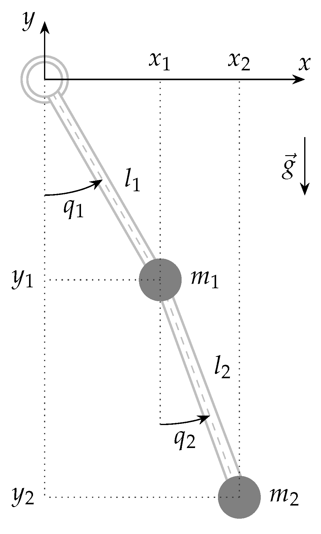
5. Linear Double Pendulum Model and Exact Solution

This section presents a case study for subsequent numerical experiments.

5.1. Lagrangian

Let us model the system depicted by Figure 1. It is a two-degree-of-freedom dynamical system composed of two masses ( m 1 , m 2 ) linked together by two massless thin rigid rods of respective fixed lengths ( l 1 , l 2 ) . Each joint articulates the system with one rotational degree of freedom. The masses’ coordinates are given by
( x 1 , y 1 ) = ( l 1 sin q 1 , l 1 cos q 1 ) ( x 2 , y 2 ) = ( l 1 sin q 1 + l 2 sin q 2 , l 1 cos q 1 l 2 cos q 2 ) ,
and their velocities are obtained by time differentiation considering that q i = q i ( t ) . The system kinetic energy is then given by
T = 1 2 m 1 x 1 ˙ 2 + y 1 ˙ 2 + 1 2 m 2 x 2 ˙ 2 + y 2 ˙ 2 ,
where an overdot indicates time differentiation. Potential energy is calculated as
V = m 1 g l 1 cos q 1 m 2 g l 1 cos q 1 + l 2 cos q 2 ,
and finally, the system Lagrangian L = T V can be explicated as
L = 1 2 ( m 1 + m 2 ) l 1 2 q 1 ˙ 2 + 1 2 m 2 l 2 2 q 2 ˙ 2 + m 2 l 1 l 2 q 1 ˙ q 2 ˙ cos ( q 1 q 2 ) + ( m 1 + m 2 ) g l 1 cos q 1 + m 2 g l 2 cos q 2 .
Small oscillations take place when q i ( t ) are small and around the stable equilibrium. This equilibrium corresponds to the system’s resting position when it is aligned with the vertical axis pointing downwards. Such motions can be described by linear equations. In this situation, the Lagrangian (44) takes a simpler form provided that the following approximations take place:
cos q 1 1 q 1 2 2 ; cos q 2 1 q 2 2 2 ; cos ( q 1 q 2 ) 1 ( q 1 q 2 ) 2 2 .
Using Equation (45), the linear form L L of Lagrangian (44) becomes
L L = 1 2 ( m 1 + m 2 ) l 1 l 1 q 1 ˙ 2 + 2 g g q 1 2 + 1 2 m 2 l 2 l 2 q 2 ˙ 2 + 2 l 1 q 1 ˙ q 2 ˙ + 2 g g q 2 2 ,
where the second term of the cos ( q 1 q 2 ) approximation in Equation (45) vanishes when multiplying the product q 1 ˙ q 2 ˙ . Generalized momenta are defined as
p i = L L q ˙ i .
According to the Lagrangian (46), we have
p 1 = ( m 1 + m 2 ) l 1 2 q 1 ˙ + m 2 l 1 l 2 q 2 ˙ , p 2 = m 2 l 2 l 1 q 1 ˙ + l 2 q 2 ˙ .
Motion equations are then obtained by applying Euler–Lagrange equations t L L q ˙ i L L q i = 0 :
( m 1 + m 2 ) l 1 2 q ¨ 1 + m 2 l 1 l 2 q ¨ 2 + ( m 1 + m 2 ) g l 1 q 1 = 0 , m 2 l 1 l 2 q ¨ 1 + m 2 l 2 2 q ¨ 2 + m 2 g l 2 q 2 = 0 .

5.2. Exact Solution

Equation (47) can also be established as a linear system of the form
M q ¨ + K q = 0 .
where
M = ( m 1 + m 2 ) l 1 2 m 2 l 1 l 2 m 2 l 1 l 2 m 2 l 2 2 ; q = q 1 q 2 ; K = ( m 1 + m 2 ) g l 1 0 0 m 2 g l 2 .
The general solution of Equation (48) is of the form
q ( t ) = Re x 1 x 2 · e i ω t ,
where x 1 and x 2 are eigenvectors and ω denotes the oscillation frequency. Two characteristic frequencies ( ω 1 , ω 2 ) are determined by the solution of the auxiliary equation det ( K ω 2 M ) = 0 :
( m 1 + m 2 ) g 2 ( m 1 + m 2 ) g ( l 1 + l 2 ) ω 2 + m 1 l 1 l 2 ω 4 = 0 .
Let us focus on the case where
l 1 = l 2 = l .
In this particular case, the oscillation frequencies are given by
ω 1 , 2 = ω 0 1 + μ r ± μ r ( 1 + μ r ) ,
with a mass ratio μ r = m 2 m 1 and frequency ω 0 = g l .
Eigenvectors x 1 and x 2 are then obtained by solving ( K ω i 2 M ) x i = 0 for i = 1 and i = 2 :
m 1 l ( 1 + μ r ) ( g ω i 2 l ) ω i 2 μ r l ω i 2 μ r l μ r ( g ω i 2 μ r l ) x i = 0 .
Solving the above system gives
x 1 = 1 1 + μ r μ r , x 2 = 1 1 + μ r μ r .
Finally, using Equation (50), the general solution of Equation (48) (or Equation (47)) can be established as
q ( t ) = c 1 x 1 cos ( ω 1 t + φ 1 ) + c 2 x 2 cos ( ω 2 t + φ 2 ) ,
where constants ( c 1 , c 2 , φ 1 , φ 2 ) are given by the chosen initial conditions on the positions and velocities.

6. Simulation Results

We will now assess the precision and convergence of our proposed integrator, previously described in Section 3. It will be compared with Newmark’s symplectic scheme, described in Section 2. Some results obtained with Runge–Kutta’s explicit fourth-order integrator, described in [3] and labeled as “RK4” throughout the rest of the document, are also given. Note that a thorough comparison with this classical integrator is beyond the scope of our contribution. The results are provided for reference since RK4 is among the most popular methods available. For benchmarking purposes, we applied these methods to the solution of the linear double pendulum (depicted by Figure 1), which has an exact solution described in the previous Section 5.
The results presented in this section are for a simulated motion of this linearized double pendulum. The computations were carried out using Wolfram’s Mathematica software (version 12.3) [33]. The figure plots were then created using exported data with the pgfplots package from . Table 1 specifies the constants and initial conditions used for all of our simulations. Using these values and following Equation (51) with null initial phases ( φ 1 , φ 2 ) , the exact solution that serves as the main reference in our comparisons is
q ex ( t ) = π 12 cos ω 1 t + cos ω 2 t 2 cos ω 1 t + cos ω 2 t ,
where ω 1 and ω 2 are given by Equation (49).
Frequency ω 0 is used to show the results in terms of an oscillation period t ¯ such that
t ¯ = 1 ω 0 .
Therefore, both the total simulation duration T and step size h are given in terms of t ¯ . It is to be noted that the presented results from Simpson’s scheme were obtained using the second variant (see Section 3.5), hence the absence of the middle value at each interpolation interval. However, both variants provided lead to the same result at each node.

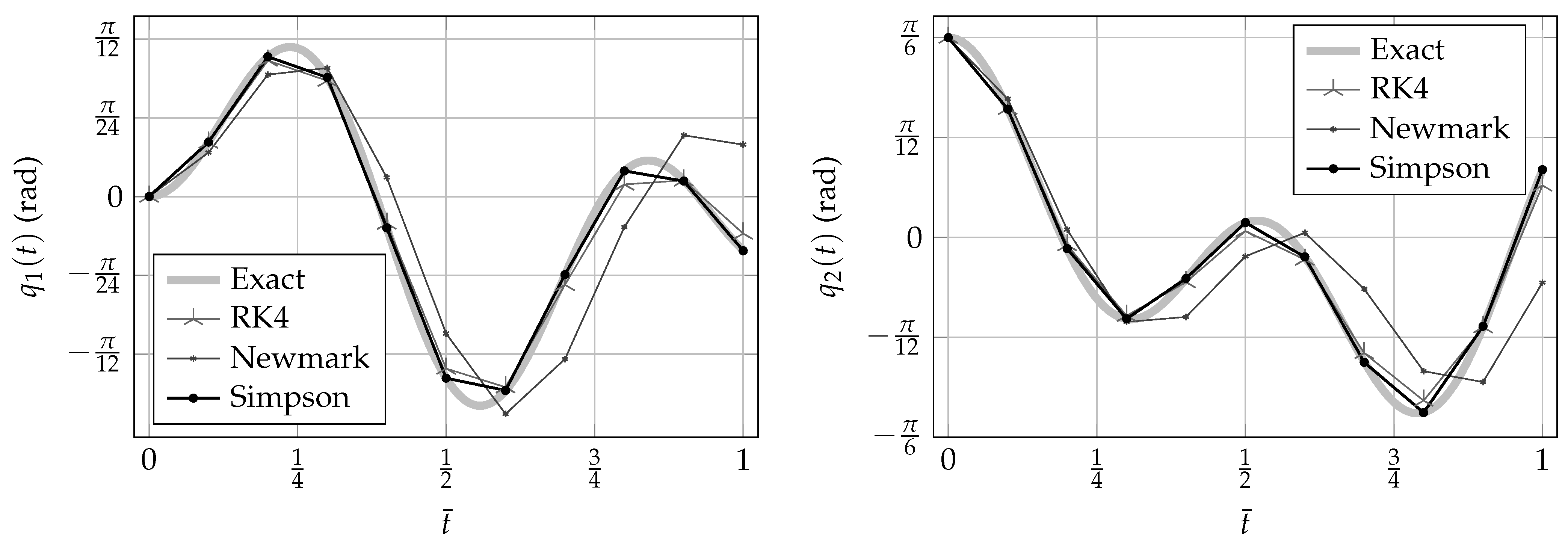
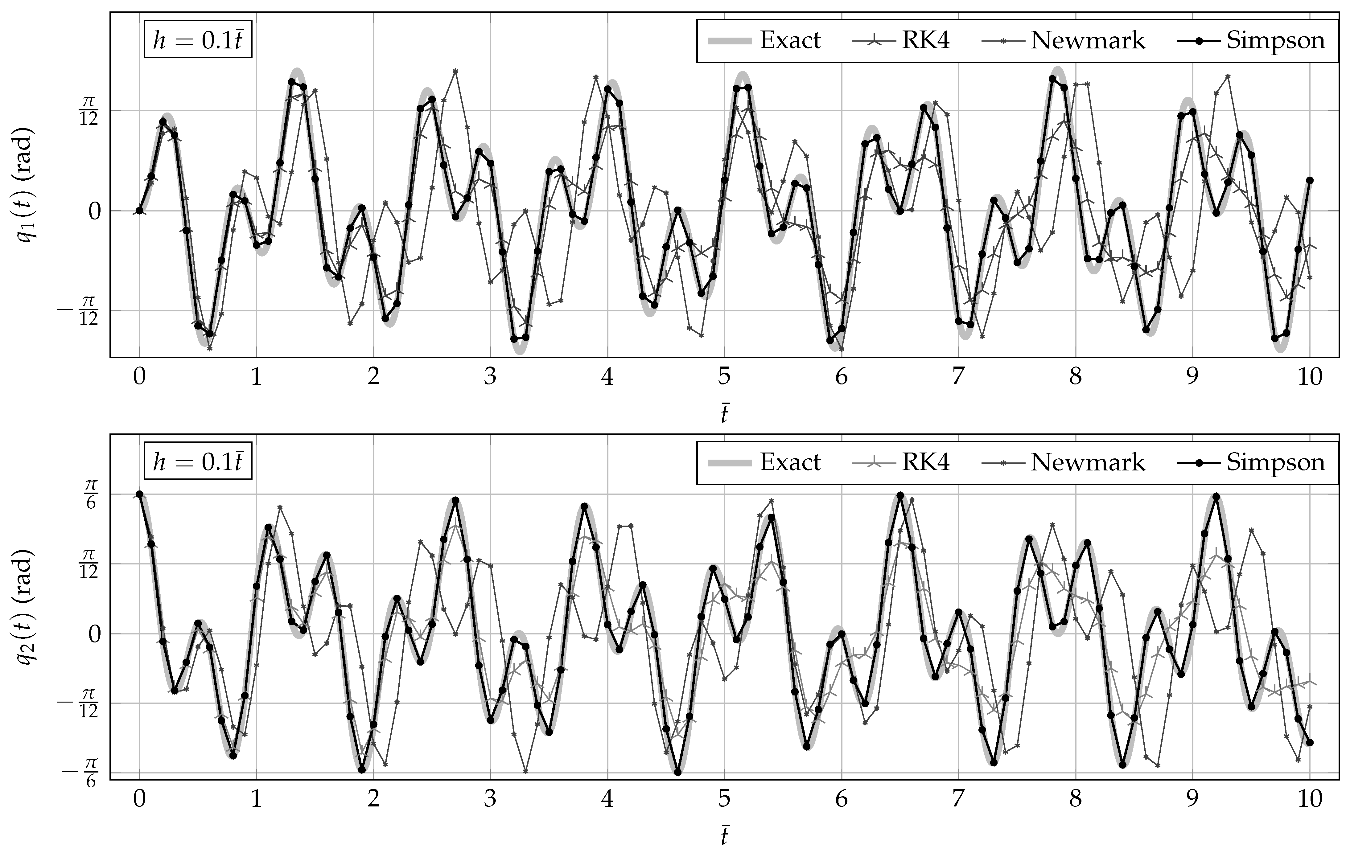
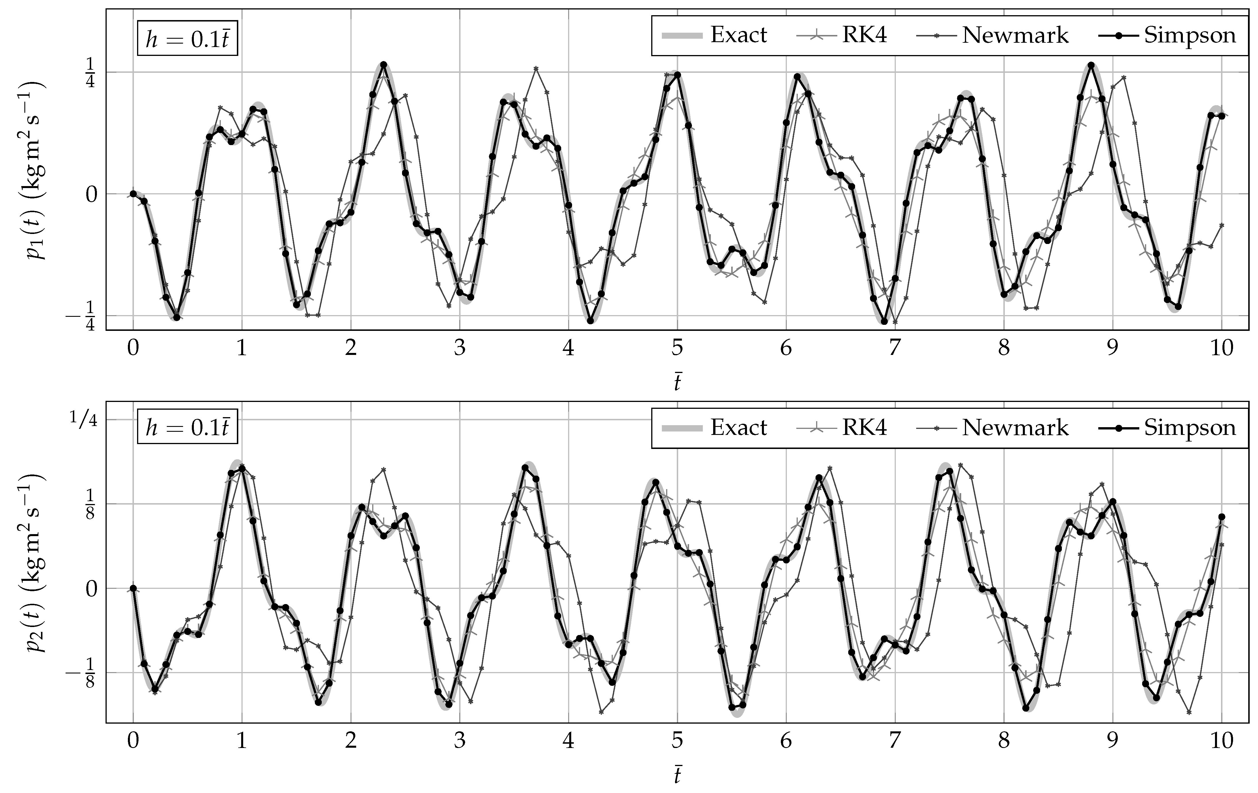
6.1. Configuration Parameters and Generalized Momenta

We begin by comparing the configuration parameter solutions q obtained with the proposed Simpson’s rule-based variational integrator, against those given by Newmark’s method. The proposed integrator uses quadratic finite elements for interpolation and Simpson’s rule (see Section 3). It is expected to be more precise than Newmark’s method, which uses a centered finite difference and the midpoint integration rule (see Section 2). Figure 2 shows the configuration parameters provided by each method, compared against the exact solution, during one period t ¯ . Simpson’s integrator is already more precise than Newmark’s scheme. Runge–Kutta’s solution is also close to the exact one, but not as much as Simpson’s solution.
Figure 2 and Figure 3 show that Simpson’s integrator is more precise than both Newmark’s and Runge–Kutta’s integrators on a short simulation ( T = 1 t ¯ ). However, Simpson’s solutions correctly follow the exact ones for longer simulations on both the configuration parameters and generalized momenta, as shown by Figure 4.
Newmark’s integrator precision can be increased by refining the step size. With h = 0.01 t ¯ , the solutions improve, but still deviate from the exact solution after a couple of periods. Simpson’s solutions correctly follow the exact solution for longer simulations.

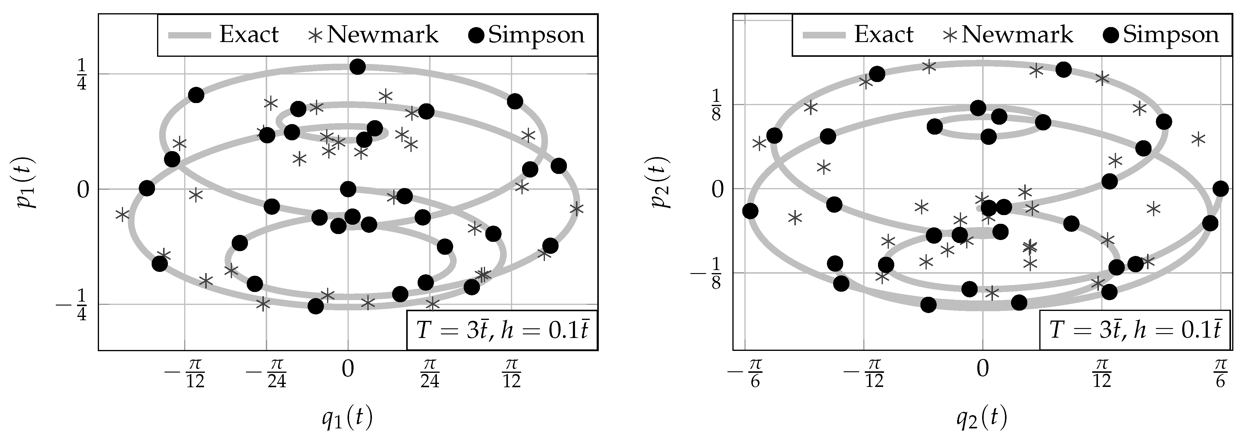
6.2. Phase Portraits

With a step size of h = 0.1 t ¯ , Newmark’s solutions’ deviations are particularly visible when tracing the motion phase portrait. Figure 5 shows the exact phase portraits topped by both Newmark’s and Simpson’s solutions. Notice how Simpson’s phase portrait clearly follows the exact one throughout the motion. The total simulation time was limited to T = 3 t ¯ for visualization purposes.

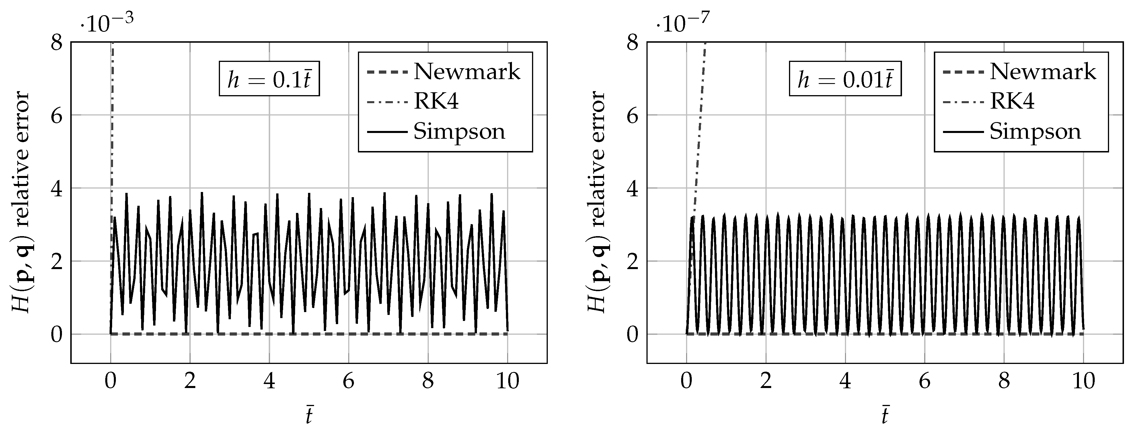
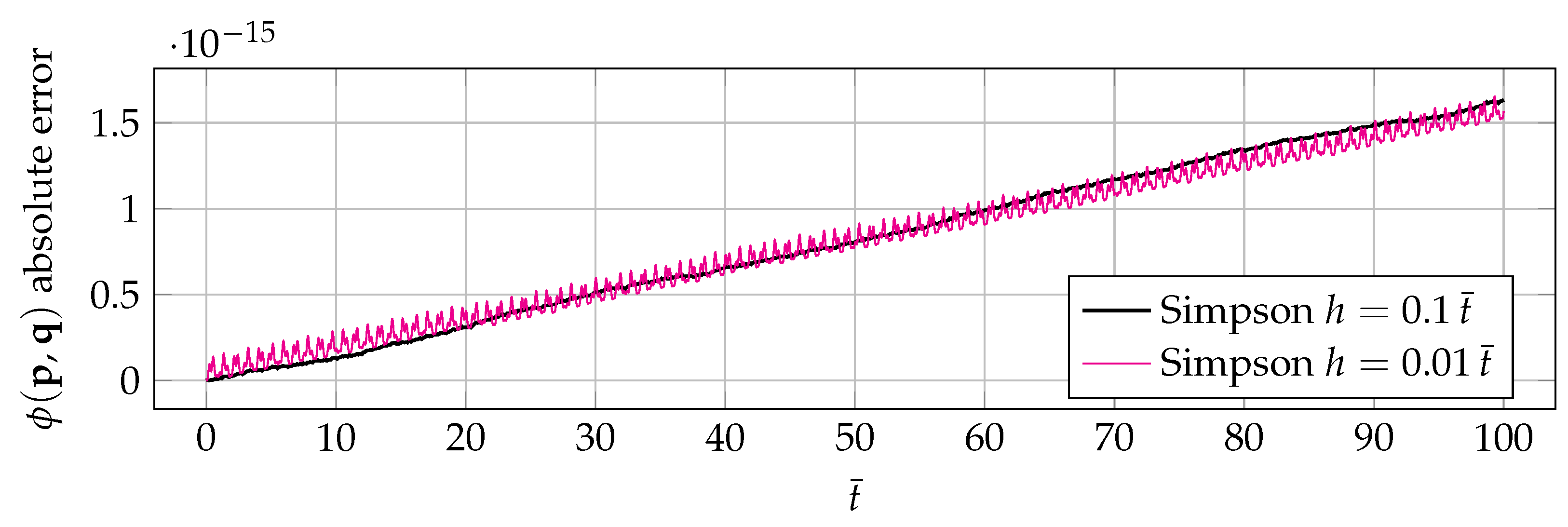
6.3. Energy Conservation
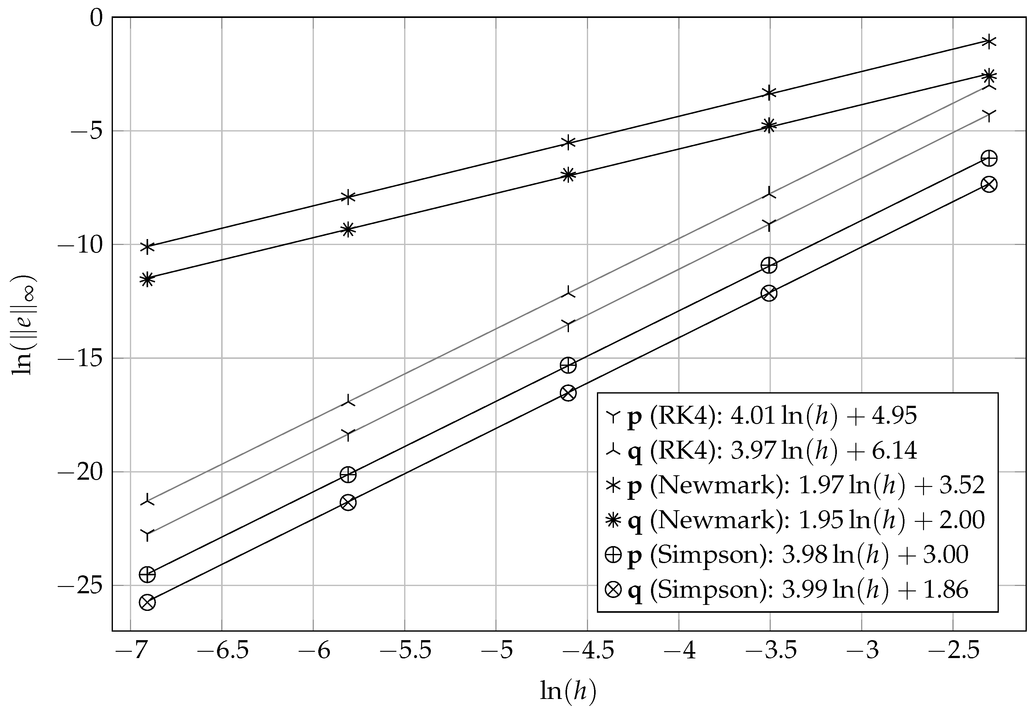
The following function gives the system energy:
H ( p , q ) = 1 2 p T M 1 p + 1 2 q T K q .
It has been previously observed (e.g., [19]) that Newmark’s integrator exactly preserves the system energy. This is not the case for our proposed integrator based on Simpson’s rule and is characteristic of most symplectic methods [19,32]. In the case of Simpson’s scheme, the second equation of System (25) introduces the small and vanishing quantity h 2 12 K q j + 1 q j h into the discrete momentum equation. Consequently, one could assume that the exact system energy may not be conserved, but a good energy behavior can be expected, as outlined in [32].
Figure 6 shows that Simpson’s solutions lead to a non-conserved energy H ( p , q ) . Nevertheless, the maximum relative error with respect to the initial value is extremely small even for h = 0.1 t ¯ , as the evaluated values are in the order of 10 3 . Notice that the energy error from Simpson’s solutions does not grow with time. Instead, it oscillates in a bounded fashion. Note that the error drops by four orders of magnitude when dividing the step size by ten (see Figure 6).
Proposition 7 shows that Simpson’s scheme preserves a quadratic form given by the function ϕ ( p , q ) of Equation (42). Matrices ξ s and ζ s (where subscript s stands for Simpson) are according to Proposition 7 as
ξ s = ( X s + Y s ) 1 = 2 h M + h 3 K L 1 1 ; ζ s = X s 1 + Y s 1 1 = 2 h M h 6 K 1 + 3 h K L 1 + 1 2 K 1 1 .
Figure 7 plots the absolute error on function ϕ ( p , q ) of Equation (42), by Simpson’s scheme. The absolute error with respect to the initial value is minimal, in the order of 10 15 , and may come from accumulated rounding errors. Note that this absolute error magnitude changes very little when refining the step size.

6.4. Convergence

The error e ( t ) = q ( t ) q ex ( t ) , and its convergence rate is measured following the prescriptions found in [16]. The schemes’ precision was evaluated using an error norm e = q q ex = sup n | q n q ex n | . Several simulations were performed for decreasing values of h between h = 0.1 t ¯ and h = 0.001 t ¯ . The e norm was calculated for each case. These errors are plotted in Figure 8, on the logarithmic scale.
Convergence rates are expressed as the power of the step size. These rates correspond to the slope of the error logarithm, as a function of the logarithm of h (see Figure 8). These trials confirmed previous analyses on Newmark’s method [17,19]: it is second-order convergent. Unsurprisingly, Runge–Kutta’s integrator is fourth-order convergent. The results also confirm the analysis performed in [26] on the convergence rate of Simpson’s scheme: it is fourth-order convergent. This rate is two degrees higher than the order of the chosen quadratic interpolation. This is known as superconvergence and is closely related to the mesh uniformity [16].
An important question is if convergence rates hold with growing simulation lengths T. Table 2 shows the convergence order evolution of Newmark’s and Simpson’s schemes with a growing simulation length, using a step size of h = 0.1 t ¯ . It can be observed that Newmark’s scheme’s convergence order decays to zero for a 1000-period simulation. RK4’s convergence rate also degrades as the simulation duration increases, although not as much as Newmark’s method. Simpson’s scheme preserves its convergence order for higher simulation periods. Error norms e are shown explicitly. Simpson’s scheme loses precision according to one order of magnitude, each time the simulation length is multiplied by ten. Table 2 exposes a normal numerical behavior of the analyzed schemes since errors accumulate over long simulations.

7. Concluding Remarks and Perspectives

In this contribution, Newmark’s method has been recalled. It is a widely used integrator in certain fields of the engineering sciences, and it is symplectic. This method has been used for benchmarking purposes in our work, where an alternative variational integrator based on Simpson’s integration rule has been proposed.
Simpson’s numerical scheme presented applies to the case of multiple-degrees of freedom systems with quadratic Lagrangians. It has been formulated linearly with partitioned matrices. The method proves to be symplectic, as demonstrated with a proof that applies to both Newmark’s and Simpson’s scheme. A sufficient stability condition on the step size was given, and it was also proven that the proposed method preserves a certain quadratic form at each time step. Simpson’s scheme is, therefore, conditionally stable.
Numerical trials on a linearized double pendulum have confirmed that the method is fourth-order accurate on both the states and generalized momenta. Numerical evaluations revealed that this convergence order is preserved for long simulations. The proposed method succeeds in predicting the evolution of dynamical systems characterized by quadratic Lagrangians.
An important extension of this work is the treatment of non-linear multi-degrees of freedom systems. In such a configuration, the middle value of the internal interpolation cannot be eliminated. This generalization should enable more applications of the proposed method, relating to Hamiltonian systems. Therefore, this is a natural objective for future developments and is currently under study. An important question relates to noise presence in matrices M and K. How would this affect the symplectic integrator? This question is relevant in the context of non-linear dynamical systems. It shall be the object of future developments as well.
A particular subject of interest relating to differential equations is the role of discrete symmetries. The analysis of discrete symmetries has many applications for finding solutions to differential equations. They can simplify a numerical scheme, as advocated in [34]. A description of finding discrete symmetries of differential equations has been given in [35]. A discrete symmetry analysis could lead to an improved symplectic integrator and is a future direction for our work.
An improved nonlinear Simpson’s variational integrator could find its application in simulating complex non-linear mechanisms. Some application examples could involve a system of synchronized pendulums [36]; the discrete optimal control of robotic systems [37]; the modal analysis of dynamical systems [38]; the motion analysis of multibody systems evolving in fluid environments [39]; or the motion prediction of sliding rods [24] and soft robots [25].

Author Contributions

Conceptualization, formal analysis, funding acquisition, methodology, project administration, resources, and visualization by J.A.R.-Q. and F.D. Software and validation by J.A.R.-Q. and J.G.C.-D. Data curation, investigation, and writing—review and editing by J.A.R.-Q., F.D. and J.G.C.-D. Writing—original draft, J.A.R.-Q. Supervision, F.D. All authors have read and agreed to the published version of the manuscript.

Funding

This research received no external funding.

Data Availability Statement

The data underlying this article will be shared upon reasonable request to the corresponding author.

Acknowledgments

This research was conducted while the corresponding author held a one-year visiting position at the Laboratoire des Sciences du Numérique de Nantes (LS2N) of the Institut Mines-Télécom (IMT) Atlantique of Nantes, France, under the authorization of CONAHCYT. The corresponding author acknowledges the support received from IMT Atlantique and CONAHCYT. The authors would like to thank the anonymous reviewers. Their valuable comments and suggestions led to considerable improvement of this article.

Conflicts of Interest

The authors declare no conflicts of interest.

References

  1. Goldstine, H.H. A History of Numerical Analysis from the 16th through the 19th Century; Studies in the History of Mathematics and Physical Sciences; Springer: New York, NY, USA, 1977. [Google Scholar] [CrossRef]
  2. Albinus, H.J. The mathematical tourist. Math. Intell. 2002, 24, 50–58. [Google Scholar] [CrossRef]
  3. Süli, E.; Mayers, D.F. An Introduction to Numerical Analysis; Cambridge University Press: Cambridge, UK, 2003. [Google Scholar]
  4. Herman, A.L.; Conway, B.A. Direct optimization using collocation based on high-order Gauss-Lobatto quadrature rules. J. Guid. Control. Dyn. 1996, 19, 592–599. [Google Scholar] [CrossRef]
  5. Kelly, M. An Introduction to Trajectory Optimization: How to Do Your Own Direct Collocation. SIAM Rev. 2017, 59, 849–904. [Google Scholar] [CrossRef]
  6. Blaszczyk, T.; Siedlecki, J.; Ciesielski, M. Numerical algorithms for approximation of fractional integral operators based on quadratic interpolation. Math. Methods Appl. Sci. 2018, 41, 3345–3355. [Google Scholar] [CrossRef]
  7. Sabir, A.; Ur Rehman, M. A numerical method based on quadrature rules for ψ-fractional differential equations. J. Comput. Appl. Math. 2023, 419, 114684. [Google Scholar] [CrossRef]
  8. Mostaghim, Z.S.; Moghaddam, B.P.; Haghgozar, H.S. Numerical simulation of fractional-order dynamical systems in noisy environments. Comput. Appl. Math. 2018, 37, 6433–6447. [Google Scholar] [CrossRef]
  9. Fakharany, M.; El-Borai, M.M.; Abu Ibrahim, M.A. Numerical analysis of finite difference schemes arising from time-memory partial integro-differential equations. Front. Appl. Math. Stat. 2022, 8, 1055071. [Google Scholar] [CrossRef]
  10. Arnold, V.I. Mathematical Methods of Classical Mechanics, 2nd ed.; Springer: New York, NY, USA, 1989. [Google Scholar]
  11. Feynman, R.P.; Hibbs, A.R. Quantum Mechanics and Path Integrals; International Series in Pure and Applied Physics; McGraw-Hill: New York, NY, USA, 1965. [Google Scholar]
  12. Souriau, J.M. Structure des Systèmes Dynamiques; Maîtrises de Mathématiques, Dunod: Paris, France, 1970. [Google Scholar]
  13. Nusser, A.; Branchini, E. On the least action principle in cosmology. Mon. Not. R. Astron. Soc. 2000, 313, 587–595. [Google Scholar] [CrossRef]
  14. Rojo, A.; Bloch, A. The Principle of Least Action: History and Physics; Cambridge University Press: Cambridge, UK, 2018. [Google Scholar]
  15. Courant, R. Variational methods for the solution of problems of equilibrium and vibrations. Bull. Am. Math. Soc. 1943, 49, 1–23. [Google Scholar] [CrossRef]
  16. Allaire, G.; Craig, A. Numerical Analysis and Optimization: An Introduction to Mathematical Modelling and Numerical Simulation; Numerical Mathematics and Scientific Computation; Oxford University Press: Oxford, UK, 2007. [Google Scholar]
  17. Newmark, N.M. A Method of Computation for Structural Dynamics. J. Eng. Mech. Div. 1959, 85, 67–94. [Google Scholar] [CrossRef]
  18. Sanz-Serna, J.M. Symplectic integrators for Hamiltonian problems: An overview. Acta Numer. 1992, 1, 243–286. [Google Scholar] [CrossRef]
  19. Kane, C.; Marsden, J.E.; Ortiz, M.; West, M. Variational integrators and the Newmark algorithm for conservative and dissipative mechanical systems. Int. J. Numer. Methods Eng. 2000, 49, 1295–1325. [Google Scholar] [CrossRef]
  20. Hairer, E.; Wanner, G.; Lubich, C. Geometric Numerical Integration; Springer Series in Computational Mathematics; Springer: Berlin/Heidelberg, Germany, 2006. [Google Scholar] [CrossRef]
  21. De Vogelaere, R. Methods of Integration which Preserve the Contact Transformation Property of the Hamilton Equations; Department of Mathematics, University of Notre Dame: Notre Dame, IN, USA, 1956. [Google Scholar] [CrossRef]
  22. Géradin, M.; Rixen, D.J. Mechanical Vibrations: Theory and Application to Structural Dynamics; John Wiley & Sons: Chichester, UK, 2015. [Google Scholar]
  23. Chopra, A.K. Dynamics of Structures: Theory and Applications to Earthquake Engineering, 5th ed.; Prentice-Hall International Series in Civil Engineering and Engineering Mechanics; Pearson Education Limited: Harlow, UK, 2020. [Google Scholar]
  24. Boyer, F.; Lebastard, V.; Candelier, F.; Renda, F. Extended Hamilton’s principle applied to geometrically exact Kirchhoff sliding rods. J. Sound Vib. 2022, 516, 116511. [Google Scholar] [CrossRef]
  25. Boyer, F.; Gotelli, A.; Tempel, P.; Lebastard, V.; Renda, F.; Briot, S. Implicit Time-Integration Simulation of Robots With Rigid Bodies and Cosserat Rods Based on a Newton–Euler Recursive Algorithm. IEEE Trans. Robot. 2024, 40, 677–696. [Google Scholar] [CrossRef]
  26. Dubois, F.; Rojas-Quintero, J.A. A Variational Symplectic Scheme Based on Simpson’s Quadrature. In Proceedings of the Geometric Science of Information, St. Malo, France, 30 August–1 September 2023; Nielsen, F., Barbaresco, F., Eds.; Springer: Cham, Switzerland, 2023; pp. 22–31. [Google Scholar] [CrossRef]
  27. Dubois, F.; Antonio Rojas-Quintero, J. Simpson’s Quadrature for a Nonlinear Variational Symplectic Scheme. In Proceedings of the International Conference on Finite Volumes for Complex Applications, Strasbourg, France, 30 October–3 November 2023; Franck, E., Fuhrmann, J., Michel-Dansac, V., Navoret, L., Eds.; Springer: Cham, Switzerland, 2023; Volume 2, pp. 83–92. [Google Scholar] [CrossRef]
  28. Raviart, P.A.; Thomas, J.M. Introduction à l’Analyse Numérique des Équations aux Dérivées Partielles; Collection Mathématiques Appliquées pour la Maîtrise; Masson: Paris, France, 1983. [Google Scholar]
  29. Gear, C. Simultaneous Numerical Solution of Differential-Algebraic Equations. IEEE Trans. Circuit Theory 1971, 18, 89–95. [Google Scholar] [CrossRef]
  30. Chyba, M.; Hairer, E.; Vilmart, G. The role of symplectic integrators in optimal control. Optim. Control. Appl. Methods 2009, 30, 367–382. [Google Scholar] [CrossRef]
  31. Razafindralandy, D.; Salnikov, V.; Hamdouni, A.; Deeb, A. Some robust integrators for large time dynamics. Adv. Model. Simul. Eng. Sci. 2019, 6, 5. [Google Scholar] [CrossRef]
  32. Zhong, G.; Marsden, J.E. Lie-Poisson Hamilton-Jacobi theory and Lie-Poisson integrators. Phys. Lett. A 1988, 133, 134–139. [Google Scholar] [CrossRef]
  33. Wolfram Research, Inc. Mathematica, version 12.3; Wolfram Research, Inc.: Champaign, IL, USA, 2021. [Google Scholar]
  34. Ibragimov, N.K. Elementary Lie Group Analysis and Ordinary Differential Equations; Wiley: Chichester, UK, 1999. [Google Scholar]
  35. Hydon, P.E. Symmetry Methods for Differential Equations: A Beginner’s Guide; Cambridge Texts in Applied Mathematics; Cambridge University Press: Cambridge, UK, 2000. [Google Scholar]
  36. Gladkov, S.O.; Bogdanova, S.B. About the possibility of synchronization in dynamical systems. J. Phys. Conf. Ser. 2020, 1479, 012011. [Google Scholar] [CrossRef]
  37. Rojas-Quintero, J.A.; Dubois, F.; Ramírez-de Ávila, H.C. Riemannian Formulation of Pontryagin’s Maximum Principle for the Optimal Control of Robotic Manipulators. Mathematics 2022, 10, 1117. [Google Scholar] [CrossRef]
  38. Shirafkan, N.; Gosselet, P.; Bamer, F.; Oueslati, A.; Markert, B.; de Saxcé, G. Constructing the Hamiltonian from the Behaviour of a Dynamical System by Proper Symplectic Decomposition. In Proceedings of the Geometric Science of Information, Paris, France, 21–23 July 2023; Nielsen, F., Barbaresco, F., Eds.; Springer: Cham, Switzerland, 2021; pp. 439–447. [Google Scholar] [CrossRef]
  39. Terze, Z.; Pandža, V.; Andrić, M.; Zlatar, D. Lie group dynamics of reduced multibody-fluid systems. Math. Mech. Complex Syst. 2021, 9, 167–177. [Google Scholar] [CrossRef]
Figure 1. Double pendulum system subject to the gravity action. The system is composed of two masses ( m 1 , m 2 ) linked together by two massless thin rigid rods of respective fixed lengths ( l 1 , l 2 ) . Each joint articulates the system with one rotational degree of freedom. Masses are located by the generalized coordinates q = ( q 1 , q 2 ) .
Axioms 13 00255 g001
Figure 2. Configuration parameters’, q , evolution for the linear double pendulum. Initial conditions are specified in Table 1. The step size is fixed as h = 0.1 t ¯ . Simpson’s integrator tracks the exact solution with more precision than Newmark’s method and Runge–Kutta’s integrator.
Axioms 13 00255 g002
Figure 3. Configuration parameters’, q , evolution for the linear double pendulum during ten periods. Initial conditions are specified in Table 1. The step size is fixed as h = 0.1 t ¯ . Simpson’s solutions correctly follow the exact solution for longer simulations.
Axioms 13 00255 g003
Figure 4. Generalized momenta’s, p , evolution for the linear double pendulum during ten periods. Initial conditions are specified in Table 1. The step size is fixed as h = 0.1 t ¯ . Simpson’s solutions correctly follow the exact solution for longer simulations.
Axioms 13 00255 g004
Figure 5. Phase portraits’ evolution for the linear double pendulum. Initial conditions are specified in Table 1. The step size is fixed as h = 0.1 t ¯ , and three periods are shown ( T = 3 t ¯ ). Simpson’s phase portrait clearly follows the exact one.
Axioms 13 00255 g005
Figure 6. As expected, the classical RK4 integrator does not preserve the system energy. Relative error grows with simulation length. Newmark’s integrator exactly preserves the system energy. Simpson’s integrator does not, but the relative error is extremely small. Notice that such an error does not grow with time, but remains bounded. The relative error drops by four orders of magnitude when dividing the step size by ten, showcasing the quality of the proposed integrator and its good energy behavior.
Axioms 13 00255 g006
Figure 7. Simpson’s scheme preserves the quadratic form ϕ ( p , q ) of Equation (42). The absolute errors are minimal and may come from accumulated rounding errors.
Axioms 13 00255 g007
Figure 8. Integrators’ convergence. The e norm was calculated for several simulations. Each simulation used a fixed step size, which was decreased from h = 0.1 t ¯ to h = 0.001 t ¯ . The convergence order corresponds to the slope of the error norm logarithm regression line. Runge–Kutta’s classical integrator convergence is in h 4 , as expected (fourth-order). Newmark’s integrator convergence is in the order of h 2 (second-order). Simpson’s integrator convergence is in the order of h 4 (fourth-order).
Axioms 13 00255 g008
Table 1. Constants and initial conditions used for numerical simulations.
ConstantsInitial Conditions
μ r = 1 q ( 0 ) = ( 0 , π 6 ) T rad
ω 0 = 2 π / s p ( 0 ) = ( 0 , 0 ) T k g m 2 / s
Table 2. Convergence order with respect to simulation length for motion simulations performed for a linearized double pendulum (see Figure 1). The initial conditions are specified in Table 1. Error norms e for momenta p and states q increase with simulation length T. Newmark’s scheme’s convergence decays to zero as T increases. RK4’s convergence rate also decays with an increasing simulation length. Simpson’s scheme preserves its convergence rate for higher simulation durations.
e Error Norm Values
Simulation Length T Number of Meshes 10 20 40 Convergence Order
t ¯ Newmark p 0.07510.02300.006061.81
RK4 p 0.01390.0008000.00005404.01
Simpson p 0.0006400.00004160.000002573.98
Newmark q 0.3420.09610.02511.88
RK4 q 0.04830.003400.0002003.91
Simpson q 0.002010.0001410.000008763.92
10  t ¯ Number of meshes100200400
Newmark p 0.2730.2060.7820.90
RK4 p 0.08220.009900.01371.29
Simpson p 0.007200.0004330.00002684.03
Newmark q 0.6940.6570.2440.75
RK4 q 0.2840.03290.01572.09
Simpson q 0.02350.001410.00009064.01
100  t ¯ Number of meshes100020004000
Newmark p 0.5210.4920.2230.61
RK4 p 0.1080.07860.006402.03
Simpson p 0.07050.004390.0002724.01
Newmark q 1.020.9640.6650.31
RK4 q 0.3280.26500.02161.96
Simpson q 0.2370.01470.0009144.01
1000  t ¯ Number of meshes10,00020,00040,000
Newmark p 0.5450.5510.5480.00
RK4 p 0.3260.1190.05951.23
Simpson p 0.1900.04380.002743.06
Newmark q 1.021.031.030.01
RK4 q 0.5810.3970.2000.77
Simpson q 0.6380.1470.009223.06
Disclaimer/Publisher’s Note: The statements, opinions and data contained in all publications are solely those of the individual author(s) and contributor(s) and not of MDPI and/or the editor(s). MDPI and/or the editor(s) disclaim responsibility for any injury to people or property resulting from any ideas, methods, instructions or products referred to in the content.

