A Method for Solving Ill-Conditioned Nonlinear Least Squares Problems and Its Application in Image Distortion Correction Using Self-Calibration

Abstract

In this study, the ill-conditioning of the iterative method for nonlinear models is discussed. Due to the effectiveness of ridge estimation for ill-conditioned problems and the lack of a combination of the H-K formula with the iterative method, the improvement of the LM algorithm is studied in this paper. Considering the LM algorithm for ill-conditioned nonlinear least squares, an improved LM algorithm based on the H-K formula is proposed for image distortion correction using self-calibration. Three finite difference methods are used to approximate the Jacobian matrix, and the H-K formula is used to calculate the damping factor in each iteration. The Brown model, quadratic polynomial model and Fourier model are applied to the self-calibration, and the improved LM algorithm is used to solve the model parameters. In the simulation experiment of space resection of a single image, we evaluate the performance of the LM algorithm based on the gain ratio (LM_h) and the improved LM algorithm based on the H-K formula (LM_HK), and the accuracy of different models and algorithms is compared. A ridge trace analysis is carried out on the damping factor to illustrate the effects of the improved algorithm in handling ill-conditioning. In the second experiment, the improved algorithm is applied to measure the diameter of a coin using a single camera. The experimental results show that the improved LM algorithm can reach the same or higher accuracy as the LM_h algorithm, and it can weaken the ill-conditioning to a certain extent and enhance the stability of the solution. Meanwhile, the applicability of the improved LM algorithm in self-calibration is verified.

1. Introduction

Self-calibration is a type of analytical calibration method that describes the system error of a camera by the distortion models in the adjustment model. The self-calibration method is convenient and flexible, and it is widely used in camera calibration. According to the coordinates of the reference points, the additional parameters in the distortion model are solved to compensate for the influence of system error on the results. In order to improve the accuracy of the self-calibration, the camera parameters and distortion parameters need to be solved accurately [1]. In the field of self-calibration, a lot of research about distortion models has been done. Based on many experiments and analyses, the Brown model was introduced into the analytical calibration method for distortion correction in 1971 [2]. Currently, the Brown model and its improved model are still commonly used in photogrammetry [3]. To address the problem of inconsistency between the optical center and the geometric center of the imaging system, self-calibration based on a simplified Brown model is proposed [4]. David et al. show that the complex distortion model can improve the accuracy of self-calibration by an experiment of three-dimensional reconstruction [5]. Based on the mathematical approximation theory, a distortion model based on the Fourier series was proposed for self-calibration purposes [6] and verified in an experiment of simulated distortion data fitting [7]. The Brown model and Fourier model are applicable in image processing, pattern classification and scene analysis in the field of computer vision. With the development of the self-calibration method, it is worth considering whether the distortion model has a strong correlation or overparameterization, which leads to ill-conditioning. Unreasonable distortion models and parameters are one of the important causes of ill-conditioning. In the self-calibration method, the quality of feature points is another important cause of ill-conditioning. It depends on many factors, including the number, accuracy and distribution of feature points [8]. Insufficient feature extraction will fail to fully reflect the role of each parameter, or unilaterally highlight the roles of some parameters. Furthermore, it is easy to cause ill-conditioning in the solution of parameters. Most of the above research avoids ill-conditioning from the aspect of model selection and feature extraction, but few research studies are carried out from the aspect of parameter iteration. In this work, the method for solving the self-calibration model is studied from the aspect of a numerical iterative method.

The solutions of ill-conditioned equations are very sensitive to small parameter value perturbations, showing poor numerical stability. For ill-conditioned equations, it is difficult to obtain accurate and reliable parameter estimates, which severely affects the accuracy and quality of data processing. For the solution of ill-conditioned problems, a variety of biased estimation methods and improved methods have been proposed to improve the quality of parameter estimates, such as regularization, truncated singular value decomposition and ridge estimation [9,10,11,12,13,14,15,16]. The key to solving ill-conditioned problems by the regularization method is the selection of the stabilization functional and regularization parameter. The stabilization functional is constructed based on prior information of the model parameters, which can effectively improve the structure of the model and make solving it feasible [17]. When prior information cannot be obtained, the stabilization functional is often expressed as a 2-norm constraint on model parameters [18] and then the ridge estimation of the parameters is derived. Ridge estimation is a special form of regularization that regards the identity matrix as a regularization matrix and then improves the reliability and stability of parameter estimation by reasonably selecting the regularization parameter. In ridge estimation, the regularization parameter is also called the ridge parameter. The common methods to determine the ridge parameters are the ridge trace method and Hoerl–Kennard (H-K) formula. After determining the appropriate ridge parameters, ridge estimation can effectively reduce the mean square error by properly modifying the ill-conditioned matrix [18]. The adjustment criterion of the ill-conditioned uncertainty model based on ridge estimation can effectively suppress the influence of ill-conditioning [19]. The common strategy for solving nonlinear parameters is to linearize the nonlinear model and solve it by an iterative method, and the Levenberg–Marquardt (LM) algorithm [20,21] is commonly used. An LM algorithm based on the gain ratio [22] can weaken the ill-conditioning by determining a damping factor, and it has been widely used in nonlinear optimization [23]. However, there are some problems in the existing research: on the one hand, the damping factor determined by this algorithm is usually large, which greatly changes the structure of the Jacobian matrix; on the other hand, although ridge estimation can effectively improve the stability of the solution, there are few research studies on the combination of ridge estimation and the LM algorithm. In response to the shortcomings of the above research work, the combination of the method for determining the ridge parameters and the LM algorithm is studied in this paper.

In this work, with the LM algorithm steps as the basic framework, an improved LM algorithm is proposed. Firstly, the ill-conditioning of the iterative method for nonlinear models is discussed. Then, according to the parameter estimation criterion of the LM algorithm, the H-K formula is combined with the LM algorithm to calculate the damping factor in each iteration. Finite difference methods are used to approximate the Jacobian matrix, and finally, we present the algorithm steps of the improved LM algorithm based on the H-K formula and finite difference. The Brown model, quadratic polynomial model and Fourier model are discussed. In the numerical experiments, the three distortion models are applied to self-calibration, and the improved LM algorithm is used to solve the model parameters. In the simulation experiment of space resection of a single image, the accuracy and performance of different models and algorithms on the solution of parameters are evaluated, and a ridge trace analysis is carried out on the damping factor to illustrate the effects of the improved algorithm in handling ill-conditioning. The applicability of the improved algorithm in practical problems is verified by the measurement of a coin diameter using a single camera. The experimental results show that the improved LM algorithm can reach the same or higher accuracy as the LM algorithm based on the gain ratio, and it can weaken the ill-conditioning to a certain extent and enhance the stability of the solution under the condition of changing the matrix structure as little as possible. The improved LM algorithm proposed in this paper provides a new method for solving self-calibration model parameters, and it also provides a new idea for solving ill-conditioned nonlinear least squares.

2. Iterative Method for Ill-Conditioned Nonlinear Least Squares Problems

2.1. Ill-Conditioned Problems in the Iterative Method

For a nonlinear model, the Taylor formula is usually used to transform it into a linear form, and then the iterative method is used to solve it. We consider a nonlinear model $\mathit{F}\left(\mathit{x}\right)={\left(F_1,F_2,\cdots ,F_m\right)}^{\mathrm{T}},\mathit{x}={\left(x_1,x_2,\cdots ,x_n\right)}^{\mathrm{T}}$, expand it by the Taylor formula and take only the first-order term:

$$\begin{array}{c}\left[\begin{array}{c}{F}_1\\ F_2\\ ⋮\\ F_m\end{array}\right]\approx \left[\begin{array}{c}{F}_1^0\\ F_2^0\\ ⋮\\ F_m^0\end{array}\right]+\left[\begin{array}{cccc}{\left.\frac{\partial F_1}{\partial x_1}\right|}_{x_1^0}& {\left.\frac{\partial F_1}{\partial x_2}\right|}_{x_2^0}& \cdots & {\left.\frac{\partial F_1}{\partial x_n}\right|}_{x_n^0}\\ {\left.\frac{\partial F_2}{\partial x_1}\right|}_{x_1^0}& {\left.\frac{\partial F_2}{\partial x_2}\right|}_{x_2^0}& \cdots & {\left.\frac{\partial F_2}{\partial x_n}\right|}_{x_n^0}\\ ⋮& ⋮& \ddots & ⋮\\ {\left.\frac{\partial F_m}{\partial x_1}\right|}_{x_1^0}& {\left.\frac{\partial F_m}{\partial x_2}\right|}_{x_2^0}& \cdots & {\left.\frac{\partial F_m}{\partial x_n}\right|}_{x_n^0}\end{array}\right]\left[\begin{array}{c}{x}_1-x_1^0\\ x_2-x_2^0\\ ⋮\\ x_n-x_n^0\end{array}\right]\hfill \\ \mathit{F}\left(\mathit{x}\right)\approx {\mathit{F}}^0+\mathit{B}\widehat{\mathit{x}}\hfill \end{array}$$

(1)

where $\mathit{B}$ is the Jacobian matrix consisting of the first-order partial derivatives of $\mathit{F}\left(\mathit{x}\right)$ at ${\mathit{x}}^0$. We rewrite it as an error equation, $\mathit{V}=\mathit{F}\left(\mathit{x}\right)-\mathit{L}\approx \mathit{B}\widehat{\mathit{x}}-\left(\mathit{L}-{\mathit{F}}^0\right)$. Under the condition of equal-precision independent observation, the iterative formula of the Gauss–Newton method can be obtained according to the least squares criterion:

$${\mathit{x}}_{k+1}={\mathit{x}}_k+{\left({\mathit{B}}_k^{\mathrm{T}}{\mathit{B}}_k\right)}^{-1}{\mathit{B}}_k^{\mathrm{T}}\left(\mathit{L}-{\mathit{F}}_k^0\right)$$

(2)

where $k$ is the number of iterations, $\mathit{B}=\left({\mathit{B}}_1,\cdots ,{\mathit{B}}_n\right)$ is a matrix of order $m\times n$ and its rank is $r$. In practical problems, usually $m>n$, and $r\left({\mathit{B}}^{\mathrm{T}}\mathit{B}\right)\le n<m$ can be obtained according to the properties of matrix rank. If $\mathit{B}$ is rank-deficient, so is ${\mathit{B}}^{\mathrm{T}}\mathit{B}$. If it is of full rank but strong multicollinearity exists in its columns:

$${\omega }_1{\mathit{B}}_1+{\omega }_2{\mathit{B}}_2+\cdots +{\omega }_n{\mathit{B}}_n\approx 0$$

(3)

where $\mathit{\omega }={\left({\omega }_1,{\omega }_2,\cdots ,{\omega }_n\right)}^{\mathrm{T}}$ is the set of eigenvectors corresponding to the eigenvalues of ${\mathit{B}}^{\mathrm{T}}\mathit{B}$. The Jacobian matrix is ill-conditioned at this moment. Rank deficiency or ill-conditioning of the matrix occurs easily when the Gauss–Newton method is used.

2.2. LM Method Based on Hoerl–Kennard Formula and Finite Differences

According to the analysis in the previous section, rank deficiency or ill-conditioning occurs easily when the Gauss–Newton method is used, resulting in no unique or stable solution in the normal equation. Therefore, to avoid the ill-posedness of the normal equation, it is necessary to impose new constraints on the parameters. L2 regularization, namely, ridge regression, is commonly used. When L2 regularization is introduced, the parameter estimation criterion and its estimation formula are

$$\begin{array}{ll}\hfill & \min \left({\mathit{V}}^{\mathrm{T}}\mathit{V}+\mu {\widehat{\mathit{x}}}^{\mathrm{T}}\widehat{\mathit{x}}\right)\hfill \\ \Rightarrow \hfill & {\mathit{x}}_{k+1}={\mathit{x}}_k+{\left({\mathit{B}}_k^{\mathrm{T}}{\mathit{B}}_k+{\mu }_k\mathit{I}\right)}^{-1}{\mathit{B}}_k^{\mathrm{T}}\left(\mathit{L}-{\mathit{F}}_k^0\right)\hfill \end{array}$$

(4)

The iterative formula for the LM method is presented as Formula (4). This is an improved algorithm based on the Gauss–Newton method, and it is also an iterative method without a specific line search for calculating the step size, which is determined by the damping factor $\mu$ [22]. The initial value of the damping factor can be set to $\mu =\tau \cdot \max \left\{B_{ii}\right\}$. $B_{ii}$ denotes the diagonal elements of ${\mathit{B}}^{\mathrm{T}}\mathit{B}$, and $\tau$ is usually a small value. If the selected initial values of the parameters are believed to be good approximations to the estimated values, it can be set to $\tau ={10}^{-6}$; otherwise, it can be set to $\tau ={10}^{-3}$ or $\tau =1$. Then, the damping factor is increased or decreased according to the gain ratio ($h$) in the iteration. The algorithm steps are as follows:

Step 1: Given the initial parameter value ${\mathit{x}}_k$, the Jacobian matrix and initial value of the damping factor are calculated, and the convergence criteria are set: the threshold ${\epsilon }_1$ of the gradient $\mathit{g}$, the threshold ${\epsilon }_2$ of the error difference and the maximum number of iterations $k_{\max }$, along with $k=0$ and $\upsilon =2$, are set.

Step 2: ${\mathit{B}}_k$ and ${\mathit{g}}_k={\mathit{B}}_k^{\mathrm{T}}\left(\mathit{L}-{\mathit{F}}_k^0\right)$ are calculated.

Step 3: The equation $\left({\mathit{B}}_k^{\mathrm{T}}{\mathit{B}}_k+{\mu }_k\mathit{I}\right){\widehat{\mathit{x}}}_k=-{\mathit{g}}_k$ is solved; then, the (k + 1)th iterative estimate is obtained: ${\mathit{x}}_{k+1}={\mathit{x}}_k+{\widehat{\mathit{x}}}_k$.

Step 4: If ${‖{\mathit{g}}_k‖}_2\le {\epsilon }_1$, ${‖{\mathit{V}}_{k+1}-{\mathit{V}}_k‖}_2\le {\epsilon }_2$, then ${\mathit{x}}_{k+1}$ is the optimal parameter estimate, and the iteration is terminated; otherwise, $h$ is calculated:

$$h=\frac{{‖{\mathit{V}}_k‖}_2^{ }-{‖{\mathit{V}}_{k+1}‖}_2^{ }}{\frac{1}{2}{\widehat{\mathit{x}}}_k^{\mathrm{T}}\left({\mu }_k{\widehat{\mathit{x}}}_k^{ }-{\mathit{g}}_k\right)}$$

Step 5: If $h>0$, then ${\mu }_{k+1}={\mu }_k\cdot \max \left\{\frac{1}{3},1-{\left(2h-1\right)}^3\right\}$ and $\upsilon =2$; otherwise, ${\mu }_{k+1}={\mu }_k\cdot \upsilon$ and $\upsilon =2\upsilon$. We set $k=k+1$ and return to Step 2.

The LM algorithm introduces the damping factor and identity matrix based on the Gauss–Newton method, which effectively resolves the rank deficiency of ${\mathit{B}}^{\mathrm{T}}\mathit{B}$ and avoids the ill-conditioning caused by multicollinearity. When the Jacobian matrix is ill-conditioned, there is at least one eigenvalue close to 0 in ${\mathit{B}}^{\mathrm{T}}\mathit{B}$, while the degree of the eigenvalue close to 0 in ${\mathit{B}}^{\mathrm{T}}\mathit{B}+\mu \mathit{I}$ will be improved, which will weaken the ill-conditioning. In the LM algorithm, the Jacobian matrix determines the descent direction of the function, and the damping factor affects both the direction and step size. Therefore, the key to solving the nonlinear model by the LM algorithm is to calculate the damping factor and the Jacobian matrix. Formula (4) shows that the calculation method of $\widehat{\mathit{x}}$ in the iterative formula can be regarded as a ridge estimation derived from the regularization principle. Therefore, different from the above method based on the gain ratio, the damping factor can be determined by the method of selecting the ridge parameter.

2.2.1. Methods for Selecting the Ridge Parameter

The damping factor is a number greater than 0, and different values lead to different ridge estimates. When $\mu \to \infty$, $\widehat{x}\to 0$, and the solution is not relevant. Therefore, the value should be chosen to be as small as possible to solve the ill-posed problem using the proximal well-posed problem. The main methods of selecting the ridge parameter are ridge trace and the Hoerl–Kennard formula.

(1)

Ridge trace: Each component ${\widehat{\mathit{x}}}_i\left(i=1,2,\cdots \right)$ of the correction value of $\mathit{x}$ is regarded as a function of the damping factor. When the damping factor changes between $\left[0,\infty \right)$, several curves can be drawn in the rectangular coordinate system $o-\mu \widehat{x}$, which are called ridge trace curves, as shown in Figure 1. With the increase in the ridge parameter, the model parameter estimates gradually stabilize and reach a stable state around $\mu \ast$. The ridge trace method selects the smallest $\mu \ast$ that makes the change stable. To determine the appropriate value according to the ridge trace curves, the following three criteria must be generally satisfied: first, the ridge estimates of model parameters in the equation are roughly stable; second, the ridge estimation can make the parameter values reasonable; and third, the sum of the squared residuals does not increase substantially. The main disadvantage of this method is the lack of a strict theoretical basis. Determining the value of the damping factor using ridge trace curves is subjective, but this subjectivity can also organically combine qualitative analysis with quantitative analysis. However, the numbers of iterations may be large. If the ridge parameter in each iteration is selected by the ridge trace curves, the workload may be large. Therefore, this method is mainly used for ridge trace analysis rather than directly determining the ridge parameter in the iteration.

(2)

Hoerl–Kennard (H-K) formula: The H-K formula is a common method for determining the ridge parameter according to the canonical form of the error equation. In order to analyze the problem, the canonical form of the error equation is introduced. Considering the symmetry of matrix ${\mathit{B}}^{\mathrm{T}}\mathit{B}$, the Formula (5) can be obtained according to matrix theory

$${\mathit{\Omega }}^{\mathrm{T}}{\mathit{B}}^{\mathrm{T}}\mathit{B}\mathit{\Omega }=\mathit{\Lambda }$$

(5)

where $\mathit{\Omega }$ is an orthogonal matrix; $\mathit{\Lambda }$ is diagonal matrix and the diagonal element is the eigenvalue of ${\mathit{B}}^{\mathrm{T}}\mathit{B}$. Formula (6) can be obtained by identity transformation of the original error equation

$$\mathit{V}=\mathit{B}\mathit{\Omega }{\mathit{\Omega }}^{\mathrm{T}}\widehat{\mathit{x}}-\left(\mathit{L}-{\mathit{F}}^0\right)$$

(6)

Denote $\mathit{C}=\mathit{B}\mathit{\Omega },\mathit{Y}={\mathit{\Omega }}^{\mathrm{T}}\widehat{\mathit{x}}$, then

$$\mathit{V}=\mathit{C}\mathit{Y}-\left(\mathit{L}-{\mathit{F}}^0\right)$$

(7)

Formula (7) is the canonical form of the error equation; $\mathit{Y}$ is the canonical parameter, and its estimation is

$$\begin{gathered} \widehat{\mathit{Y}}={\left({\mathit{C}}^{\mathrm{T}}\mathit{C}\right)}^{-1}{\mathit{C}}^{\mathrm{T}}\left(\mathit{L}-{\mathit{F}}^0\right) \\ ={\mathit{\Lambda }}^{-1}{\mathit{C}}^{\mathrm{T}}\left(\mathit{L}-{\mathit{F}}^0\right)\hspace{1em}\hspace{0.17em} \end{gathered}$$

(8)

According to $\widehat{\mathit{x}}=\mathit{\Omega }\mathit{Y}$, the parameter estimation of the original error equation can be obtained. In canonical form, the mean square error (MSE) of the canonical parameter is

$$\begin{gathered} MSE\left(\mathit{Y}\right)=E\left({‖\widehat{\mathit{Y}}-\mathit{Y}‖}^2\right) \\ \hspace{1em}\hspace{1em}\hspace{1em}\hspace{1em}\hspace{1em}\hspace{1em}\hspace{1em}\hspace{0.17em}=E\left({‖{\left({\mathit{C}}^{\mathrm{T}}\mathit{C}\right)}^{-1}{\mathit{C}}^{\mathrm{T}}\mathit{V}‖}^2\right) \\ \hspace{1em}\hspace{1em}\hspace{1em}\hspace{1em}\hspace{1em} =E\left({\mathit{V}}^{\mathrm{T}}\mathit{C}{\mathit{\Lambda }}^{-2}{\mathit{C}}^{\mathrm{T}}\mathit{V}\right) \end{gathered}$$

(9)

Hoerl and Kennard proposed the H-K formula [14] based on the canonical form of the error equation. $\left({\mathit{\omega }}_1,\cdots ,{\mathit{\omega }}_n\right)$ are assumed to be the eigenvectors corresponding to the eigenvalues $\left({\lambda }_1,\cdots ,{\lambda }_n\right)$ of ${\mathit{B}}^{\mathrm{T}}\mathit{B}$:

$$\begin{array}{cc}\mathit{\Omega }=\left({\mathit{\omega }}_1,\cdots ,{\mathit{\omega }}_n\right),& \mathit{\Lambda }=\mathrm{diag}\left({\lambda }_1,\cdots ,{\lambda }_n\right)\end{array}$$

(10)

Then $\mu$ is calculated by the H-K formula

$$\mu =\frac{{\widehat{\sigma }}^2}{\max {\widehat{e}}_i^2}$$

(11)

where ${\widehat{\sigma }}^2=\frac{{\mathit{V}}^{\mathrm{T}}\mathit{V}}{m-n}$ and $\widehat{\mathit{e}}={\mathit{\Lambda }}^{-1}\mathit{\Omega }{\mathit{B}}^T\left(\mathit{L}-\mathit{F}\right)={\left({\widehat{e}}_1,\cdots ,{\widehat{e}}_n\right)}^{\mathrm{T}}$. Then

$$\widehat{\mathit{x}}={\left({\mathit{B}}^{\mathrm{T}}\mathit{B}+\mu \mathit{I}\right)}^{-1}{\mathit{B}}^{\mathrm{T}}\left(\mathit{L}-{\mathit{F}}_{ }^0\right)$$

(12)

The mean square error of parameter estimation is

$$MSE\left(\widehat{\mathit{x}}\right)={\sigma }^2{\displaystyle \sum _{i=1}^r\frac{{\lambda }_i}{{\left({\lambda }_i+\mu \right)}^2}}+{\mu }^2{\displaystyle \sum _{i=1}^r\frac{{\mathit{x}}_i^2}{{\left({\lambda }_i+\mu \right)}^2}}$$

(13)

It can be seen that, when $\mu$ is large, although this estimation method can overcome the multicollinearity, it will also introduce more bias. The determination of $\mu$ according to the H-K formula is related to the eigenvalues. An ill-conditioned matrix contains very small eigenvalues, so a smaller value can be obtained according to the H-K formula, so that the parameter estimation can be stable as soon as possible with less bias.

2.2.2. Finite Difference Form of the Jacobian Matrix

The Jacobian matrix can be calculated according to the differentiation rule of functions of several variables, as expressed in Formula (1). However, in practical problems, due to the large number of observation equations and the associated large-scale matrices, this method may require a huge amount of calculation. In a common numerical method, the finite difference approximates the differential of the function by the corresponding function value after parameter discretization. This method of approximating the derivative by the difference quotient can effectively reduce the calculational burden. In this paper, the forward difference method (FDM), backwards difference method (BDM) and central difference method (CDM) are adopted to approximate the Jacobian matrix. According to the definition of forward difference, $\mathrm{\Delta }{F}_i=F_i\left(x_j+\delta \right)-F_i\left(x_j\right)$, and $\delta$ is the difference step. $F_i\left(x_j+\delta \right)$ is expanded by the Taylor formula, and only the first-order term is considered:

$$\begin{array}{c}{F}_i\left(x_j+\delta \right)\approx F_i\left(x_j\right)+\frac{\partial F_i}{\partial x_j}\left(x_j+\delta -x_j\right)\\ \frac{\partial F_i}{\partial x_j}\approx \frac{F_i\left(x_j+\delta \right)-F_i\left(x_j\right)}{\delta }\end{array}$$

(14)

Similarly, the backwards difference and central difference are

$$\begin{array}{l}\frac{\partial F_i}{\partial x_j}\approx \frac{F_i\left(x_j\right)-F_i\left(x_j-\delta \right)}{\delta }\\ \frac{\partial F_i}{\partial x_j}\approx \frac{F_i\left(x_j+\delta \right)-F_i\left(x_j-\delta \right)}{2\delta }\end{array}$$

(15)

Compared with the forward difference and backwards difference, the accuracy of approximating the Jacobian matrix by the central difference is higher, and the calculational burden is multiple times larger.

The steps of the improved LM algorithm based on the H-K formula and finite differences are as follows:

Step 1: Given an initial parameter value ${\mathit{x}}_k$, set convergence criteria: the threshold ${\epsilon }_1$ of gradient $\mathit{g}$, the threshold ${\epsilon }_2$ of the error difference and the maximum number of iterations $k_{\max }$, along with $k=0$, are set.

Step 2: Given the difference step, $\frac{\partial F_i}{\partial x_j}\left(i=1,\cdots ,m,j=1,\cdots ,n\right)$ is calculated by the finite difference method, the matrix ${\mathit{B}}_k$ is obtained, and ${\mathit{g}}_k={\mathit{B}}_k^{\mathrm{T}}\left(\mathit{L}-{\mathit{F}}_k^0\right)$ is calculated; then, the damping factor is determined by the H-K formula ${\mu }_k=\frac{{\widehat{\sigma }}^2}{\max {\widehat{e}}_i^2}$.

Step 3: The equation $\left({\mathit{B}}_k^{\mathrm{T}}{\mathit{B}}_k+{\mu }_k\mathit{I}\right){\widehat{\mathit{x}}}_k=-{\mathit{g}}_k$ is solved, and the (k + 1)th parameter estimate ${\mathit{x}}_{k+1}={\mathit{x}}_k+{\widehat{\mathit{x}}}_k$ is obtained.

Step 4: If ${‖{\mathit{g}}_k‖}_2\le {\epsilon }_1$, ${‖{\mathit{V}}_{k+1}-{\mathit{V}}_k‖}_2\le {\epsilon }_2$, then ${\mathit{x}}_{k+1}$ is the optimal parameter estimate, and the iteration is terminated; otherwise, we set $k=k+1$ and return to Step 2.

2.3. Distortion Models

In photogrammetry, since the beam of the imaging system within the field of view does not strictly meet the ideal center projection, the actual image points produce a position error, which is called distortion. Considering the distortion of image points, the actual image coordinates can be regarded as the sum of the ideal image coordinates and distortion, which is expressed by a collinearity equation with additional parameters:

$$\begin{array}{c}u=-f\frac{R_{11}\left(X - X_S\right) + R_{21}\left(Y - Y_S\right) + R_{31}\left(Z - Z_S\right)}{R_{13}\left(X - X_S\right) + R_{23}\left(Y - Y_S\right) + R_{33}\left(Z - Z_S\right)} + u_0 + \mathrm{\Delta }u\\ v=-f\frac{R_{12}\left(X - X_S\right) + R_{22}\left(Y - Y_S\right) + R_{32}\left(Z - Z_S\right)}{R_{13}\left(X - X_S\right) + R_{23}\left(Y - Y_S\right) + R_{33}\left(Z - Z_S\right)} + v_0 + \mathrm{\Delta }v\end{array}$$

(16)

where $\left(u,v\right)$ are the actual image coordinates, $\left(X,Y,Z\right)$ are the corresponding ground control point coordinates, $\left(u_0,v_0,f\right)$ are the elements of interior orientation, $\left(X_S,Y_S,Z_S\right)$ are the translation elements of exterior orientation, $R_{ij}\left(i,j=1,2,3\right)$ are the direction cosine composed of the angle elements of exterior orientation $\left({\phi }_1,{\phi }_2,{\phi }_3\right)$ and $\left(\mathrm{\Delta }u,\mathrm{\Delta }v\right)$ are the distortions, which are generally functions of the image coordinates. Formula (16) is also called a self-calibration model. Distortion models mainly include physical models and mathematical models. The Brown model, polynomial model and Fourier model are mainly described in this paper.

2.3.1. Brown Model

The Brown model is a commonly used physical model, which was originally designed for large-area film cameras. Various forms of distortion that occur in camera imaging are considered. In practical applications, the parameters of the Brown model need to be selected according to the camera imaging characteristics. With the application of a digital camera in aerial photography, the model has been simplified into radial distortion and decentering distortion. The Brown model is expressed as

$$\begin{array}{c}\mathrm{\Delta }{u}_{\mathrm{Radial}}=\overline{u}\left(K_1{s}^2+K_2{s}^4+K_3{s}^6\right)\\ \mathrm{\Delta }{v}_{\mathrm{Radial}}=\overline{v}\left(K_1{s}^2+K_2{s}^4+K_3{s}^6\right)\\ \\ \mathrm{\Delta }{u}_{\mathrm{Decentring}}=2P_1\overline{u}\overline{v}+P_2\left(r^2+{\overline{u}}^2\right)\\ \mathrm{\Delta }{v}_{\mathrm{Decentring}}=2P_2\overline{u}\overline{v}+P_1\left(r^2+{\overline{v}}^2\right)\end{array}$$

(17)

where $s=\sqrt{{\overline{u}}^2+{\overline{v}}^2}$, and $K_i\left(i=1,2,3\right)$ and $P_i\left(i=1,2\right)$ are radial distortion parameters and decentering distortion parameters. The distortion of the image edges can be described only by the radial distortion and decentering distortion when using a digital camera. In practical applications, radial distortion usually remains $K_1,K_2$.

2.3.2. Polynomial Model and Fourier Model

In addition to the physical model, the distortion model can also be established from the mathematical point of view (in this section, $a$ is used to represent the distortion coefficient of different mathematical models). The orthogonal polynomial in the mathematical model can effectively reduce the correlation between parameters and improve the stability of the solution. The polynomial model is a commonly used distortion correction model, which is expressed mathematically as

$$\begin{array}{c}\mathrm{\Delta }u={\displaystyle \sum _{i=0}^t{\displaystyle \sum _{j=0}^{t-i}{a}_{ij}{\overline{u}}^i{\overline{v}}^j}}\\ \mathrm{\Delta }v={\displaystyle \sum _{i=0}^t{\displaystyle \sum _{j=0}^{t-i}{a}_{ij}{\overline{u}}^i{\overline{v}}^j}}\end{array}$$

(18)

where $t$ is the order of the polynomial and $a_{ij}$ are the parameters to be determined. However, a higher-order polynomial is also prone to overparameterization, which will not only increase the calculational work required to obtain the numerical solution but also lead to the instability of the solution. Therefore, the order should not be too high in practical applications. The quadratic polynomial (QP) model is often selected as a distortion model. Considering the correlation of the coefficients in $u$ and $v$, the quadratic orthogonal polynomial model is

$$\begin{array}{l}\mathrm{\Delta }{u}_{\mathrm{QP}}=a_{10}\overline{u}+a_{01}\overline{v}-a_{20}{\overline{u}}^2+a_{11}\overline{u}\overline{v}+a_{02}{\overline{v}}^2\\ \mathrm{\Delta }{v}_{\mathrm{QP}}=-a_{01}\overline{v}+a_{10}\overline{u}+a_{11}\overline{u}\overline{v}-a_{02}{\overline{v}}^2+a_{20}{\overline{u}}^2\end{array}$$

(19)

According to the Weierstrass second approximation theory, a binary Fourier series orthogonal polynomial model represented by the image coordinates can be obtained [6]:

$$\begin{array}{l}\mathrm{\Delta }u=a_1{\mathrm{COS}}_{1,0}+a_2{\mathrm{COS}}_{0,1}+a_3{\mathrm{COS}}_{1,-1}+a_4{\mathrm{COS}}_{1,1}+a_5{\mathrm{SIN}}_{1,0}+a_6{\mathrm{SIN}}_{0,1}+a_7{\mathrm{SIN}}_{1,-1}+a_8{\mathrm{SIN}}_{1,1}\\ \mathrm{\Delta }v=a_9{\mathrm{COS}}_{1,0}+a_{10}{\mathrm{COS}}_{0,1}+a_{11}{\mathrm{COS}}_{1,-1}+a_{12}{\mathrm{COS}}_{1,1}+a_{13}{\mathrm{SIN}}_{1,0}+a_{14}{\mathrm{SIN}}_{0,1}+a_{15}{\mathrm{SIN}}_{1,-1}+a_{16}{\mathrm{SIN}}_{1,1}\end{array}$$

(20)

where $a_i$ are the parameters to be determined and ${\mathrm{COS}}_{i,j}=\cos \left(i\overline{u}+j\overline{v}\right),{\mathrm{SIN}}_{i,j}=\sin \left(i\overline{u}+j\overline{v}\right)$, $\overline{u}=\frac{\left(u-\mathrm{width}/2\right)}{\mathrm{width}}\pi ,\overline{v}=\frac{\left(v-\mathrm{height}/2\right)}{\mathrm{height}}\pi$ (width and height are the image width and height).

3. Numerical Experiments and Analysis

The first experiment involves a simulation experiment of the space resection of a single image based on the collinearity equation with additional parameters, and the second involves measuring the diameters of coins using a single camera. The improved LM algorithm is used in the numerical experiments, and the convergence conditions are set as follows:

$$\left.\begin{array}{l}{‖{\mathit{g}}_k‖}_2\le {10}^{-5}\hfill \\ {‖{\mathit{V}}_{k+1}-{\mathit{V}}_k‖}_2\le {10}^{-5}\hfill \\ k_{\max }=50\hfill \end{array}\right\}$$

(21)

The Jacobian matrix in each iteration is approximated by the finite difference methods introduced in Section 2. The H-K formula is used to calculate the damping factor, which is compared with the method according to the gain ratio. The experimental environment is MATLAB R2021a running on a 1.80 GHz PC with Windows 7.

3.1. Space Resection of a Single Image Based on the Collinearity Equation with Additional Parameters

In this experiment, the image points in a single aerial image are simulated for space resection. It is assumed that the local coordinate system is a North-East-Down (NED) coordinate system, the flight altitude is 50 m, the design focal length of the camera is 9 mm, the pixel size is $2.4 \mathsf{\mu }\mathrm{m}/\mathrm{px}$ and the image width and height are 5472 pixels and 3648 pixels. At the moment of exposure, the focal length is 8.9 mm, the coordinates of the principal points are $u_0=2737.2 \mathrm{px}, v_0=1827.4 \mathrm{px}$ and the elements of exterior orientation are $X_{\mathrm{S}}=5 \mathrm{m}, Y_{\mathrm{S}}=-10 \mathrm{m}, Z_{\mathrm{S}}=-51 \mathrm{m}, {\phi }_1=0°, {\phi }_2=1°, {\phi }_3=2°$. This experiment is carried out according to the following steps:

Step 1: Simulate the data. The values of $X$ and $Y$ of the ground points are centered on the plane coordinates of the camera station, which are uniformly distributed in the range of $\left[X_S-10,X_S+10\right]$ and $\left[Y_S-10,Y_S+10\right]$. And the values of $Z$ are in the range of [−1, 1] since the origin of the NED coordinate system is set on the ground. A total of 120 image coordinates, and the corresponding ground point coordinates, are simulated, and Gaussian noises are added to the image coordinates as observations.

Step 2: Select the distortion models. The Brown model, quadratic polynomial (QP) model and Fourier model are regarded as distortion models, which are added to the collinearity equation to form the self-calibration models.

Step 3: Initialization. The initial values of the angle elements of the exterior orientation are set to ${\phi }_1={\phi }_2={\phi }_3=0°$, the initial value of $Z_{\mathrm{S}}$ is $Z_{\mathrm{S}}^0=-50 \mathrm{m}$ and the initial values of $X_{\mathrm{S}}$ and $Y_{\mathrm{S}}$ are calculated according to the following formula

$$X_{\mathrm{S}}^0=\frac{{\displaystyle \sum _{i=1}^m{X}_i}}{m},Y_{\mathrm{S}}^0=\frac{{\displaystyle \sum _{i=1}^m{Y}_i}}{m}$$

where $m$ is the number of ground points. The initial values of the elements of the interior orientation are $u_0^0=\mathrm{width}/2,v_0^0=\mathrm{height}/2,f^0=9\mathrm{mm}$, and the initial values of the additional parameters are set to 0. The normalized image coordinates are substituted into the self-calibration models composed of the three distortion models.

Step 4: Solve the parameters. The LM algorithm based on the forward difference, backwards difference and central difference methods with the gain ratio and the H-K formula (LM_FDM+h, LM_BDM+h, LM_CDM+h, LM_FDM+HK, LM_BDM+HK and LM_CDM+HK) are used to solve the parameters. The elements of the interior orientation, and additional parameters, are determined while solving for the elements of the exterior orientation.

The experiment evaluates the performance of the algorithms from the following aspects: the accuracy is compared using the sum of squared residuals (SSR), the maximum residuals of the image points, the reprojection errors (REs) and the true errors of the parameters; the efficiency is compared using the number of iterations and the running time; the influence on the ill-conditioning is compared using the condition number; the stability of the solution is analyzed using the ridge trace curve.

Table 1. SSR and maximum residuals of each algorithm.

	Models	Brown		QP		Fourier
Algorithms		SSR	Maximum	SSR	Maximum	SSR	Maximum
LMFDM+h		$1.631\times {10}^{-4}$	$3.137\times {10}^{-4}$	$1.114\times {10}^{-4}$	$2.990\times {10}^{-4}$	$6.245\times {10}^{-6}$	$3.511\times {10}^{-4}$
LMBDM+h		$1.632\times {10}^{-4}$	$3.137\times {10}^{-4}$	$1.114\times {10}^{-4}$	$2.990\times {10}^{-4}$	$6.245\times {10}^{-6}$	$3.511\times {10}^{-4}$
LMCDM+h		$1.631\times {10}^{-4}$	$3.137\times {10}^{-4}$	$1.114\times {10}^{-4}$	$2.990\times {10}^{-4}$	$6.245\times {10}^{-6}$	$3.511\times {10}^{-4}$
LMFDM+HK		$3.197\times {10}^{-6}$	$3.423\times {10}^{-4}$	$3.145\times {10}^{-6}$	$3.391\times {10}^{-4}$	$2.856\times {10}^{-6}$	$2.959\times {10}^{-4}$
LMBDM+HK		$3.197\times {10}^{-6}$	$3.423\times {10}^{-4}$	$3.145\times {10}^{-6}$	$3.391\times {10}^{-4}$	$2.856\times {10}^{-6}$	$2.959\times {10}^{-4}$
LMCDM+HK		$3.196\times {10}^{-6}$	$3.423\times {10}^{-4}$	$3.144\times {10}^{-6}$	$3.391\times {10}^{-4}$	$2.856\times {10}^{-6}$	$2.958\times {10}^{-4}$

presents the SSR and the maximum residuals of each algorithm at the optimal solution. It can be seen from Table 1 that, for the same algorithm, the fitting accuracy of different models for image coordinate observations is high, and the SSR of the Fourier model is generally the smallest, reaching an accuracy of ${10}^{-6}$. Because the three difference methods are consistent in the approximation of the Jacobian matrix, the difference between the results obtained by the three difference methods is small. In contrast, the performance of the LM algorithm based on CDM is better. For the maximum residuals obtained by the LM algorithm based on the gain ratio (LM_h) and the improved LM algorithm based on the H-K formula (LM_HK), there is no significant law, which means that the LM_HK algorithm has a poor fitting effect on image points with a large error. However, the SSR corresponding to the LM_HK algorithm is generally smaller, reaching an accuracy of ${10}^{-6}$, indicating that the LM_HK algorithm has a higher fitting accuracy for the observations. According to the introduction of the H-K formula in Section 2, the H-K formula can determine a small damping factor and less bias is introduced, so that the solution of the parameters can reach a higher accuracy. This is proved by the comparison results of the LM_h algorithm and LM_HK algorithm. Through the above analysis, another discovery obtained from the table is explained: for the same model, the LM_CDM+HK algorithm can reach the same or higher accuracy as other algorithms.

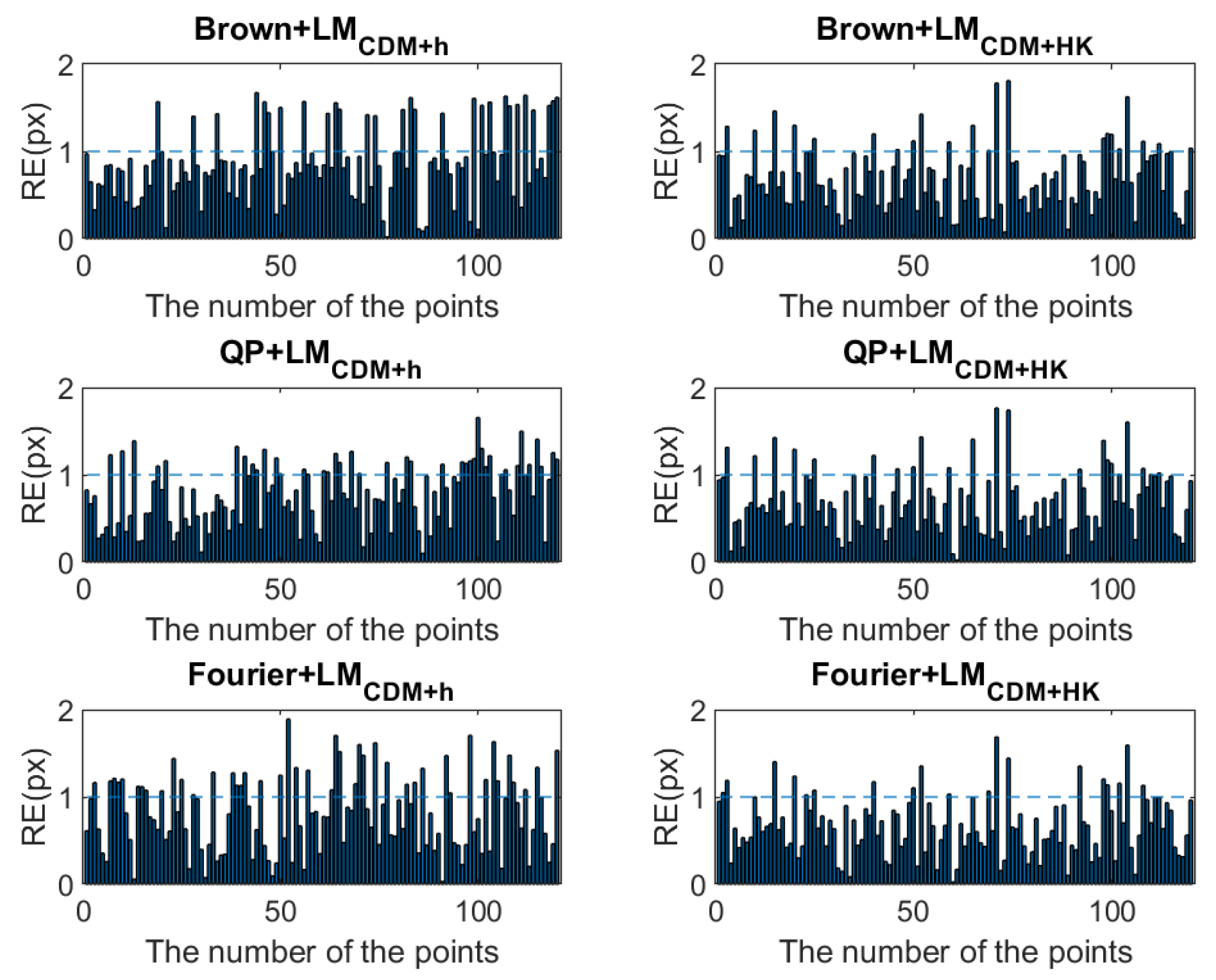
The LM algorithm based on CDM shows a better performance in Table 1. Therefore, in order to show the accuracy of the improved LM algorithm more clearly and intuitively, Figure 2 and

Table 2. The RMSE of reprojection errors (px).

	Models	Brown	QP	Fourier
Algorithms
LMCDM+h		0.970	0.861	0.929
LMCDM+HK		0.937	0.861	0.749

present the distribution and the root mean square error (RMSE) of reprojection errors (REs) obtained by the LM_CDM+h and LM_CDM+HK corresponding to each model. In Figure 2, the dotted line indicates the position where the RE is 1 pixel. It can be seen from Figure 2 that the maximum of the REs for all methods is less than 2 pixels. For the same model, the number of image points with an RE greater than 1 pixel in the results of the LM_CDM+HK algorithm is generally less than that of the LM_CDM+h algorithm, and a consistent conclusion can be obtained from Table 2: the RMSE corresponding to the LM_CDM+HK algorithm is the same as or smaller than that of the LM_CDM+h algorithm, which indicates that the LM_CDM+HK algorithm can reach the same or higher accuracy as the LM_CDM+h algorithm. For the same algorithm, the RMSE of the Brown model is the closest to 1 pixel, which is the worst accuracy of all the methods. The Brown model considers radial distortion and decentering distortion without considering other forms of distortion. The QP model and Fourier model, established from the perspective of function approximation, can accurately fit the unknown distortion in the image. The accuracy of the Fourier model solved by the LM_CDM+HK algorithm is less than 0.8 pixels, which is the highest accuracy of all methods.

Table 3. The true errors of parameters.

	Methods	LMCDM+h			LMCDM+HK
Errors		Brown	QP	Fourier	Brown	QP	Fourier
$\mathrm{\Delta }{X}_{\mathrm{S}}\left(\mathrm{m}\right)$		0.065	0.064	0.064	0.002	−0.010	−0.051
$\mathrm{\Delta }{Y}_{\mathrm{S}}\left(\mathrm{m}\right)$		0.766	0.755	0.745	0.017	−0.015	−0.008
$\mathrm{\Delta }{Z}_{\mathrm{S}}\left(\mathrm{m}\right)$		0.721	0.776	0.998	−0.573	0.572	−0.206
$\mathrm{\Delta }{\varphi }_1\left(\mathrm{rad}\right)$		$-1.824\times {10}^{-3}$	$-1.730\times {10}^{-3}$	$-2.106\times {10}^{-3}$	$-4.841\times {10}^{-4}$	$-1.392\times {10}^{-4}$	$-1.746\times {10}^{-3}$
$\mathrm{\Delta }{\varphi }_2\left(\mathrm{rad}\right)$		$1.661\times {10}^{-2}$	$1.610\times {10}^{-2}$	$8.391\times {10}^{-3}$	$1.067\times {10}^{-3}$	$4.340\times {10}^{-4}$	$7.422\times {10}^{-3}$
$\mathrm{\Delta }{\varphi }_3\left(\mathrm{rad}\right)$		$1.506\times {10}^{-4}$	$5.104\times {10}^{-4}$	$-2.008\times {10}^{-2}$	$-1.005\times {10}^{-5}$	$-9.283\times {10}^{-6}$	$-7.342\times {10}^{-3}$
$\mathrm{\Delta }f\left(\mathrm{px}\right)$		41.665	41.665	41.666	41.588	41.652	41.696
$\mathrm{\Delta }{u}_0\left(\mathrm{px}\right)$		−1.200	−1.199	−1.199	−1.803	−1.248	−1.206
$\mathrm{\Delta }{v}_0\left(\mathrm{px}\right)$		−3.399	−3.399	−3.399	−3.376	−3.358	−3.434

presents the true errors of the parameters. It can be seen from Table 3 that the parameter estimates of LM_CDM+h and LM_CDM+HK have an equivalent accuracy. From the true error of the exterior orientation elements, it can be found that, compared with the LM_CDM+h, the true error obtained by the LM_CDM+HK is generally smaller and the result is closer to the true value.

Figure 3 shows the iterative changes in the SSR for different models solved by LM_CDM+h and LM_CDM+HK. In order to clearly show the difference, the first iteration has been removed.

Table 4. The number of iterations k and the running time (s).

	Models	Brown		QP		Fourier
Algorithms		k	Time	k	Time	k	Time
LMFDM+h		14	3.681	12	1.647	8	2.459
LMBDM+h		14	3.666	12	1.632	8	2.508
LMCDM+h		14	7.224	12	3.204	8	4.963
LMFDM+HK		5	1.313	5	0.728	5	1.609
LMBDM+HK		5	1.348	5	0.739	5	1.580
LMCDM+HK		5	2.601	5	1.411	5	3.302

presents the number of iterations and the running time of each algorithm and model. According to Table 4, the number of iterations and the running time of the LM_HK algorithm are generally less than those of the LM_h algorithm, indicating that a high fitting accuracy can be obtained by the improved algorithm, with a higher iterative efficiency. According to the running time, compared with the LM_CDM+h algorithm, the efficiency of the LM_CDM+HK algorithm is improved by 64%, 55% and 33% corresponding to the three models. The algorithms using CDM to approximate the Jacobian matrix require more time, which is consistent with the principle of central difference. Compared with FDM and BDM, CDM needs to calculate one more approximate partial derivative of each variable in the iteration within the difference step range, and the calculational burden is the largest. As shown in Figure 3, the LM_CDM+h algorithm makes the SSR of the Brown model reach a stable state after five iterations, which indicates that the descending speed is slower. However, the LM_CDM+HK algorithm makes the SSR of all models stable after three iterations.

To further analyze the performance of the improved LM algorithm based on the H-K formula, a ridge trace analysis of the different methods is carried out. Figure 4 shows the ridge trace curves of $\widehat{\mathit{x}}$ changing with the damping factor at the optimal solution.

Table 5. The condition number and damping factor at the optimal solution.

	Models	Brown		QP		Fourier
		C0	$\mathit{\mu }$	C0	$\mathit{\mu }$	C0	$\mathit{\mu }$
Algorithms		C		C		C
LMCDM+h		$7.263\times {10}^{16}$	4.028	$2.705\times {10}^{17}$	3.373	$2.113\times {10}^{15}$	$3.586\times {10}^{-3}$
		26.823		32.576		$1.233\times {10}^5$
LMCDM+HK		$1.179\times {10}^{13}$	$5.698\times {10}^{-9}$	$3.684\times {10}^{17}$	$6.407\times {10}^{-8}$	$2.777\times {10}^{15}$	$2.752\times {10}^{-9}$
		$1.918\times {10}^{10}$		$1.707\times {10}^9$		$1.633\times {10}^{11}$

shows the condition number (C/C₀) of the normal matrix with or without the damping factor. It can be seen from Table 5 that both the LM_CDM+h algorithm and the LM_CDM+HK algorithm can reduce the condition number of the matrix and weaken the ill-conditioning, and the effect of the LM_CDM+h algorithm is more significant. Especially for the Brown model and the QP model, the condition number is reduced to 26.823 and 32.576, which can be considered to mean that the matrix is well-posed. However, it can be seen from Figure 4 that the order of magnitude of the damping factor for the Brown model, QP model and Fourier model should be ${10}^{-9}$, ${10}^{-14}$ and ${10}^{-11}$. According to the selection principle of the damping factor and Table 5, the actual value determined by the LM_CDM+h algorithm is generally too large, while the values of damping factor determined by the LM_CDM+HK algorithm are relatively consistent with the trend of the ridge trace curves, which is closer to the result of the ridge trace analysis. Therefore, it is found that the LM_CDM+h algorithm weakens the ill-conditioning of the normal matrix more significantly, since this algorithm changes the structure of the normal matrix by selecting a larger damping factor. Upon the premise of changing the structure of the normal matrix as little as possible, the LM_CDM+HK algorithm can weaken the ill-conditioning to a certain extent and make the solution stable by selecting a smaller damping factor.

3.2. Measurement of a Coin Diameter Using a Single Camera

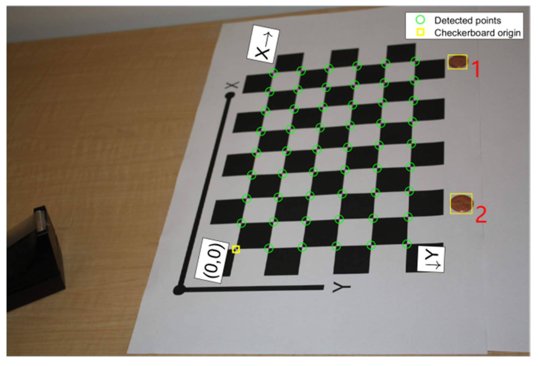
Experiment 3.1 shows that the LM algorithm based on CDM presents a better performance in solving the self-calibration model. Therefore, LM_CDM+h and LM_CDM+HK are used to measure the diameters of coins using a single camera in this experiment. Nine images of a calibration pattern are taken from different angles to calibrate the camera by Zhang’s calibration method. Taking the calibration result as the initial value and using the detected point of the last image, LM_CDM+h and LM_CDM+HK are combined with the Brown model, QP model and Fourier model to estimate the model parameters and then measure the diameters of the coins. The detected points and the coins are shown in Figure 5. The SSR and the maximum residuals in pixels of each algorithm and model are shown in

Table 6. SSR and maximum residuals (px).

	Models	Brown		QP		Fourier
Algorithms		SSR	Maximum	SSR	Maximum	SSR	Maximum
LMCDM+h		$8.512\times {10}^{-3}$	$2.738\times {10}^{-2}$	$1.208\times {10}^{-5}$	$9.448\times {10}^{-3}$	$1.816\times {10}^{-4}$	$3.617\times {10}^{-3}$
LMCDM+HK		$8.950\times {10}^{-3}$	$2.858\times {10}^{-2}$	$1.007\times {10}^{-5}$	$8.995\times {10}^{-3}$	$9.463\times {10}^{-5}$	$3.137\times {10}^{-3}$

.

It can be seen from Table 6 that the accuracy of all the models and algorithms is high, since good initial values are obtained. The SSR and maximum residuals of the LM_CDM+h algorithm and LM_CDM+HK algorithm are consistent, which indicates that the fitting accuracy is equivalent. The orders of magnitude of SSR and the maximum for the Brown model are ${10}^{-3}$ and ${10}^{-2}$. For the same algorithm, the accuracy of the Brown model is lower, while the accuracy of the QP model and Fourier model are higher, which indicates that the image has other forms of distortion except radial distortion and decentering distortion, and the mathematical model can compensate for these distortions more effectively.

Table 7. The number of iterations k and the running time (s).

	Models	Brown		QP		Fourier
Algorithms		k	Time	k	Time	k	Time
LMCDM+h		8	1.569	6	2.213	6	2.350
LMCDM+HK		7	1.378	4	1.587	4	1.622

presents the number of iterations and running time. It can be seen from Table 7 that the LM_CDM+HK algorithm has a higher iteration efficiency than LM_CDM+h. This is consistent with the conclusion in Section 3.1. According to the running time, the efficiency of the LM_CDM+h algorithm is improved by 12%, 28% and 30% corresponding to the three models. For the same algorithm, the QP model and Fourier model need fewer iterations, while the Brown model requires more iterations. However, the running time of the Brown model is the least, since the model has the least number of distortion parameters.

To measure the coins, the top-left and top-right corners of the bounding box are converted into world coordinates. Then the Euclidean distance between them is calculated in millimeters. The actual diameter is 19.05 mm. The diameters of the coins calculated by different methods are shown in

Table 8. The diameter of coins calculated by different methods (mm).

	Models	Brown		QP		Fourier
Algorithms		Diameter1	Diameter2	Diameter1	Diameter2	Diameter1	Diameter2
LMCDM+h		19.054	18.886	19.053	18.886	19.053	18.886
LMCDM+HK		19.053	18.886	19.053	18.887	19.053	18.887

. It can be seen from Table 8 that the numerical results calculated by the different methods are consistent. The measurements of the first coin and the second coin are accurate to within 0.004 mm and 0.164 mm. All the methods have a sufficiently high accuracy.

4. Discussion

In this work, we study the combination of the H-K formula and the LM algorithm, and an analysis of the LM algorithm and its improvement are carried out in the numerical experiment. Consistent with the previous study [20,21,22,23], it is found that the LM algorithm based on the gain ratio (LM_h) is effective in handling nonlinear least squares problems, and it can weaken the ill-conditioning of the Jacobian matrix by determining the damping factor. However, from the perspective of ridge estimation, the damping factor determined by this algorithm is generally too large, and it greatly changes the structure of the matrix. In the existing literature about the methods for solving ill-conditioning [9,10,11,12,13,14,15,16,17,18,19], there is no research on the combination of the H-K formula and the LM algorithm. Therefore, an improved LM algorithm based on the H-K formula (LM_HK) is proposed and used to solve the self-calibration model composed of the Brown model, QP model and Fourier model.

From the numerical experiment and analysis, it is found that, compared with the LM_h algorithm, the LM_HK algorithm can reach the same or higher accuracy, and it makes the SSR stable after fewer calculations (three iterations) in the simulation experiment, indicating that a high fitting accuracy can be reached by the improved algorithm with a higher iterative efficiency. In the ridge trace analysis, it is found that the damping factor determined by the improved LM algorithms is smaller, and it is consistent with the trend of the ridge trace curves, which means that this algorithm can weaken the ill-conditioning to a certain extent and make the solution stable by selecting a smaller damping factor and changing the structure of the Jacobian matrix as little as possible.

From the aspect of the distortion model, we consider the fitting effects of the Brown model, QP model and Fourier model on image distortion. In this paper, the study of the Brown model is different from the previous study [2,4]. In the simulation experiment, the specific distortion form is uncertain. Under this condition, the fitting effect of the Brown model on distortion is studied. It is found that if there are unknown distortions in the image, the mathematical model, such as the QP model and Fourier model, can effectively compensate for these distortions. For the same algorithm, the fitting accuracy of the Fourier models for image point observations is higher, which is consistent with the previous study [7].

Although the study reveals the above discoveries, there are also limitations in this paper. In this paper, the LM algorithm is improved from the perspective of ridge estimation. However, in addition to the ridge trace method and H-K formula, the method for determining the ridge parameters also includes the minimum mean square error and cross validation, which are not considered. Therefore, an important future direction for improving the LM algorithm is a combination of the calculation of the damping factor and other methods for determining the ridge parameter.

5. Conclusions

Ill-conditioning generally exists in nonlinear least squares problems. An LM algorithm based on the gain ratio is the commonly used method, and it is discussed in this paper. This algorithm linearizes the nonlinear model and weakens the ill-conditioning of the Jacobian matrix by determining a damping factor. However, the damping factor determined by this algorithm is usually large, which greatly changes the structure of the matrix. Since the H-K formula can weaken the ill-conditioning by determining a smaller damping factor, an improved LM algorithm based on the H-K formula is proposed for solving nonlinear least squares problems. From the perspective of the ridge estimation of nonlinear parameters, the damping factor is calculated by the H-K formula. For the ill-conditioned problem in image distortion, the Brown model, quadratic polynomial model and Fourier model are discussed for the space resection of a single image. The improved LM algorithm based on the H-K formula is used to solve the self-calibration model, and it is applied to measure the diameter of coins using a single camera. The applicability of the improved LM algorithm in self-calibration is verified. Through numerical experiments, it is found that the improved LM algorithm can stabilize the parameter values under the condition of changing the matrix structure as little as possible, and it can reach the same or a higher accuracy than the LM algorithm based on the gain ratio. The improved LM algorithm based on the H-K formula provides a new method for solving the self-calibration model, and it also provides a new idea for solving ill-conditioned nonlinear least squares.

References

1. Huang, W.; Jiang, S.; Liu, X.Z.; Jiang, W. GNSS Constrained Self-Calibration for Long Corridor UAV Image. Geomat. Inf. Sci. Wuhan Univ. 2024, 49, 197–207. [Google Scholar] [CrossRef]
2. Brown, D.C. Close-range camera calibration. Photogramm. Eng. 1971, 37, 855–866. [Google Scholar] [CrossRef]
3. Sun, P. Research on Key Techniques of Large Scale Dynamic Photogrammetry; Beijing University of Posts and Telecommunications: Beijing, China, 2019. [Google Scholar]
4. Gao, Z.Y.; Gu, Y.Y.; Liu, Y.H.; Xu, Z.B.; Wu, Q.W. Self-calibration based on Simplified Brown Nonlinear Camera Model and Modified BFGS Algorithm. Opt. Precison Eng. 2017, 25, 2532–2540. [Google Scholar] [CrossRef]
5. David, G.; Helene, B. Comparison of pre- and self-calibrated camera calibration models for UAS-derived nadir imagery for a SfM application. Prog. Phys. Geogr. Earth Environ. 2018, 43, 215–235. [Google Scholar] [CrossRef]
6. Tang, R.; Fritsch, D.; Cramer, M. New Rigorous and Flexible Fourier Self-calibration Models for Airborne Camera Calibration. ISPRS J. Photogramm. Remote Sens. 2012, 71, 76–85. [Google Scholar] [CrossRef]
7. Sun, J.M.; Yu, J.P.; Li, J.M.; Man, Y.Y.; Shen, G. Performance Analysis of a Generic Photogrammetric Distortion Model. Spacecr. Recovery Remote Sens. 2020, 41, 110–117. [Google Scholar]
8. Bian, Y.; Wang, M.; Chu, Y.; Liu, Z.; Chen, J.; Xia, Z.; Fang, S. A Cost Function for the Uncertainty of Matching Point Distribution on Image Registration. Int. J. Geo-Inf. 2021, 10, 438. [Google Scholar] [CrossRef]
9. Tikhonov, A.N.; Arsenin, V.Y. Solutions of Ill-Posed Problems; John Wiley & Sons: New York, NY, USA, 1977. [Google Scholar] [CrossRef]
10. Hansen, P.C. The Truncated SVD as a Method for Regularization. BIT Numer. Math. 1987, 27, 534–553. [Google Scholar] [CrossRef]
11. Park, Y.; Reichel, L.; Rodriguez, G. Parameter determination for Tikhonov regularization problems in general form. J. Comput. Appl. Math 2018, 343, 12–25. [Google Scholar] [CrossRef]
12. Aravkin, A.Y.; Drusvyatskiy, D.; van Leeuwen, T. Efficient quadratic penalization through the partial minimization technique. IEEE Trans. Autom. Control. 2018, 63, 2131–2138. [Google Scholar] [CrossRef]
13. Guo, H.; Liu, G.; Wang, L. An Improved Tikhonov-Regularized Variable Projection Algorithm for Separable Nonlinear Least Squares. Axioms 2021, 10, 196. [Google Scholar] [CrossRef]
14. Hoerl, A.E.; Kennard, R.W. Ridge Regression: Applications to Nonorthogonal Problems. Technometrics 1970, 12, 69–82. [Google Scholar] [CrossRef]
15. Li, B.F.; Shen, Y.Z.; Feng, Y.M. Fast GNSS Ambiguity Resolution as an Ill-posed Problem. J. Geod. 2010, 84, 683–698. [Google Scholar] [CrossRef]
16. Lin, D.F.; Yao, Y.B.; Zheng, D.Y.; Li, C.K. Determination of Truncation Parameter based on the Differences of TSVD Parameter Estimates for Ill-posed Problems in Geodesy. Acta Geod. Cartogr. Sin. 2022, 51, 1787–1796. [Google Scholar]
17. Xu, X.Y.; Li, J.C.; Wang, Z.T.; Zou, X.C. The Simulation Research on the Tikhonov Regularization Applied in Gravity Field Determination of GOCE Satellite Mission. Acta Geod. Cartogr. Sin. 2010, 39, 465–470. [Google Scholar] [CrossRef]
18. Lin, D.F.; Zhu, J.J.; Song, Y.C. Construction Method of Regularization by Singular Value Decomposition of Design Matrix. Acta Geod. Cartogr. Sin. 2016, 45, 883–889. [Google Scholar]
19. Lu, T.D.; Wu, G.M.; Zhou, S.J. Ridge estimation algorithm to ill-posed uncertainty adjustment model. Acta Geod. Cartogr. Sin. 2019, 48, 403–411. [Google Scholar] [CrossRef]
20. Levenberg, K.Q. A method for the solution of certain nonlinear problems in least squares. Q. J. Appl. Math. 1944, 2, 164–168. [Google Scholar] [CrossRef]
21. Marquardt, D.W. An algorithm for the least-squares estimation of nonlinear parameters. J. Soc. Ind. Appl. Math. 1963, 11, 431–441. [Google Scholar] [CrossRef]
22. Madsen, K.; Nielsen, H.B.; Tingleff, O. Methods for Non-Linear Least Squares Problems, 2nd ed.; Society for Industrial & Applied Mathematics; Informatics and Mathematical Modelling, Technical University of Denmark: Kongens Lyngby, Denmark, 2004. [Google Scholar] [CrossRef]
23. Yang, G.C.; Wang, Q.; Yu, B.G.; Liu, P.; Li, S. High-precision indoor positioning based on robust LM visual inertial odometer and pseudosatellite. Acta Geod. Cartogr. Sin. 2022, 51, 18–30. [Google Scholar] [CrossRef]
Figure 1. Diagram of ridge trace curves.
Axioms 13 00209 g001
Figure 2. The distribution of reprojection errors.
Axioms 13 00209 g002
Figure 3. Iterative changes of SSR in different methods.
Axioms 13 00209 g003
Figure 4. Ridge trace curves of x ^ at the optimal solution.
Axioms 13 00209 g004
Figure 5. The detected points and the coins.
Axioms 13 00209 g005