Abstract
In this paper, we present a survey about the latest results in global stability concerning the discrete-time evolutionary Ricker competition model with n species, in both, autonomous and periodic models. The main purpose is to convey some arguments and new ideas concerning the techniques for showing global asymptotic stability of fixed points or periodic cycles in these kind of discrete-time models. In order to achieve this, some open problems and conjectures related to the evolutionary Ricker competition model are presented, which may be a starting point to study global stability, not only in other competition models, but in predator–prey models and Leslie–Gower-type models as well.
Keywords:
discrete dynamical systems; periodic evolutionary; Ricker competition model; local stability; global stability; mixed monotone maps MSC:
39A23; 39A30; 39A60; 37N25
1. Introduction
Using the idea of Darwinian evolution [], Jim Cushing together with some coworkers established the foundation of discrete phenotype evolutionary models in a series of papers [,,,,,,]. These models are based on evolutionary game theory, which is ruled by three axioms: variation in trait values, fitness differences, and inheritance.
Clearly, evolutionary game models differ from classical games. While classical games prioritize strategies that optimize players’ payoffs, evolutionary games prioritize strategies that endure over time. Through births and deaths, players come and go. However, their strategies pass on from generation to generation [].
In 2019, Ackleh et al. [] studied the local properties of a discrete-time predator–prey model. The authors established conditions for the existence and stability of the equilibrium points, and conditions for the persistence of the prey and predator populations in both non-evolutionary and evolutionary models. It is shown that the evolution of toxicant resistance allows both predator and prey to persist when, without evolution, both would go extinct.
In [], Elaydi et al. studied the effect of evolution in the autonomous Ricker competition model of two species. The authors studied the local stability of the fixed points and the effect of the evolution in the new model. The theoretical results indicated that evolution can promote and/or suppress the stability of the coexistence equilibrium depending on the environment. In the case of destabilization, complex dynamics occur and may lead to either a period-doubling bifurcation, as in the non-evolutionary Ricker equation, or to a Neimark–Sacker bifurcation. This phenomenon does not happen in the non-evolutionary model.
In [], K. Mokni et al. studied the asymptotic stability and presented a bifurcation analysis on a discrete evolutionary Ricker-type population model with immigration. In [], the authors studied a new approach to a special class of discrete-time evolutionary models and established a solid mathematical theory to analyze them. The authors also proposed a new evolutionary competition model for both single and multiple species using the strategy of evolutionary game theory.
Finally, in [], M. Ch-Chaoui and K. Mokni presented a derivation of a discrete-time evolutionary Beverton–Holt model. The authors discussed the existence of the positive fixed point and explored its asymptotic stability. They also showed that, under certain parameter conditions, the Neimark–Sacker bifurcation is present, which is a phenomenon that does not occur in the non-evolutionary model.
The above-mentioned studies are essentially focused on local stability and bifurcation for autonomous models and mostly for single species.
Dealing with global stability in discrete models is a real challenge even for simple models. In the case of evolutionary models, Elaydi et al., in [], were able to show global stability in a Ricker-type model, in both autonomous and periodic cases, by using the idea of mixed monotone maps, which were firstly studied by Kulenovic and Merino in [] and later popularized by H. Smith in [,].
The study of global stability presented in [] for the evolutionary Ricker-type model is far from complete since there are a large number of cases, depending on the parameters, where the authors were not able to show global stability.
Hence, the main goal of this paper is to convey some open problems and conjectures concerning the evolutionary Ricker competition model for n species (see Section 4) and promote discussion among researchers in order to develop new techniques for showing global asymptotic stability for fixed points or periodic cycles. In Section 2, we present the state of the art concerning the single-species evolutionary Ricker model. The main findings in both autonomous and periodic evolutionary Ricker-type models for one species are described. In Section 3, we explore the latest developments in the multi-species Ricker competition model. In particular, we present some results concerning the global stability in the model with n species with a single trait.
2. Single-Species Evolutionary Ricker Model
In a recent paper [], Elaydi et al. studied the global dynamics of the following evolutionary Ricker model of a single species x (with a single mean trait u and individual trait v):
where is the sequence of growth rates (which are functions of the trait v), is the competition coefficient (which depends on both the individual’s trait v and the trait u), is the speed of evolution (which is proportional to the constant variance of the individual trait v), and the coefficient is the sensitivity of the competition.
Notice that the first equation in (1) is the inherent fertility equation, while the second equation is the trait equation, more widely known in the literature as the canonical equation for evolution [], i.e., Lande’s equation [,] or Fisher’s equation [].
The details of the derivation of Model (1) when , for all , i.e., the autonomous model, may be found in Cushing [] and in Elaydi et al. [].
The global dynamics of the non-trivial fixed point (in the autonomous case) and of the non-trivial periodic cycle (in the non-autonomous periodic case) are accomplished by the idea of mixed monotone mappings introduced by Hal Smith in []. The following result is the main theorem in [] concerning the global dynamics of the autonomous single-species Ricker model (1):
Theorem 1
(Global asymptotic stability). Let for all such that , , and . Then, the interior equilibrium point of Model (1) is globally asymptotically stable if it is locally asymptotically stable, where .
Remark 1.
The conditions of local stability required in Theorem 1 are
and
with , and as stated in Theorem 2.1 in [].
Figure 1 illustrates a region given by the two above conditions, in the parameter space.
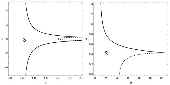
Figure 1.
Representation of the local stability region S of the interior fixed point of Model (1) in the parameter space bifurcation diagram. In S, the conditions of local stability given in Remark 1 are satisfied for . In the left figure, , while in the right figure, . When the parameters cross the curves (solid and dashed), a bifurcation occurs. The period-doubling bifurcation occurs when the parameters cross the dashed curve, whereas the Neimark–Sacker bifurcation appears when the parameters cross the solid curve. The fixed point loses stability and a new phenomenon is born.
Concerning the non-autonomous periodic case, i.e., when for all and some integer , Elaydi et al. [] showed that the origin is a saddle fixed point of periodic System (1) when and there exits a periodic cycle of the form
that is globally asymptotically stable when and .
Furthermore, by using a new definition of an associated map, Elaydi et al. were able to show that non-autonomous p-periodic System (1) is mixed monotone. Thus, from a perturbation result, the following theorem was proved:
Theorem 2
(Global asymptotic stability of the 2-periodic system). Let for all such that , , and . Then, for sufficiently small and letting , there is a 2-periodic cycle that is globally asymptotically stable in the interior of the first quadrant if and in the interior of the fourth quadrant if .
Remark 2.
A generalization of the previous result is stated in Theorem 3.9 in [] for general period p.
3. Multi-Species Ricker Competition Model
The Ricker competition model of n species is given by
where , for , represents the population size of the species at time unit t. The parameters , for , are the inherent growth rates at low densities, and the coefficients are the competition intensity coefficients that measure the effects of intraspecific competition and interspecific competition. More precisely, are the intraspecific competition parameters, while , for , are the interspecific competition parameters. Notice that these parameters are assumed to be positive.
When , for all and , Model (2) is autonomous, whereas when for some and integer , Model (2) is periodic.
The local properties and the bifurcation scenario of the fixed points of the mapping representing Model (2) may be found in [] when and in [] when . An illustration of the stability regions is provided in Figure 2 for and in Figure 3 for .
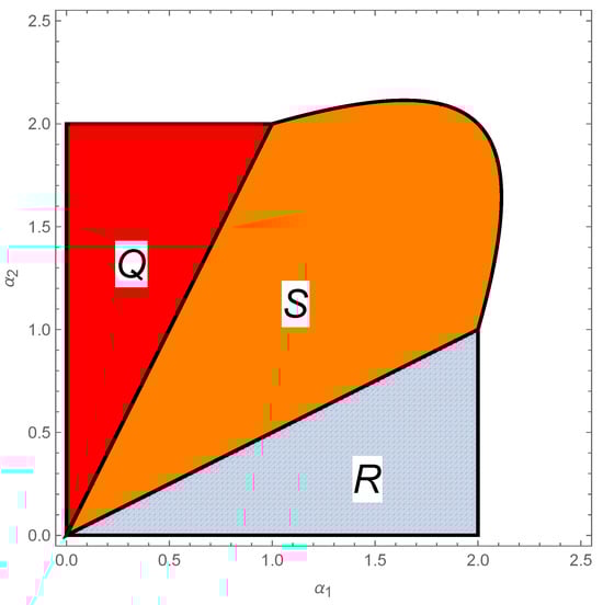
Figure 2.
Representation of the stability regions Q, S, and R of the equilibrium points in the two-species Ricker competition model (2) when and in the parameter space . In region R, the fixed point on the axis is locally asymptotically stable, with a period-doubling bifurcation at and , with as a bifurcation parameter. In region Q, the equilibrium point on the axis is locally asymptotically stable, with a period-doubling bifurcation at and , with as a bifurcation parameter. In region S, the interior fixed point is locally asymptotically stable. On the curve (a hyperbola), a period-doubling bifurcation occurs with respect to the parameters and .
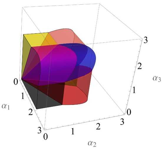
Figure 3.
Stability regions of the seven non-trivial fixed points of the 3D autonomous Ricker competition model (2) in the parameter space , when for and for . Details about these regions may be found in [].
The global stability of the non-trivial fixed points of Model (2) is a real challenge even in the autonomous case and this subject is far from being concluded. There are some studies for some particular situations.
When the autonomous model is considered, studies of the global asymptotic stability of the planar Ricker competition model can be found in [,,,], for the three-dimensional model, in [], and for the higher dimension, in []. We should mention that the global stability in the higher dimension is accomplished when Model (2) is monotone.
In the context of periodic situations, there is a scarcity of studies. As far as we know, the only one present in the literature for the periodic planar Ricker Model is [] when the model is monotone.
In a similar way, following Cushing’s methodology used in the single-species case, we can establish the following evolutionary Ricker competition model for n species with a single mean trait and individual trait :
The parameters are as before, such that , , , and for all .
Notice that the inherent fertility equations are
while Lande’s equations or Fisher’s equations are
Now, firstly considering the autonomous system, i.e., when for all and all and setting and , System (3) may be represented by the map given by
The mapping F possesses a large number of fixed points, namely, the origin O; fixed points of the form
where , for is the canonical basis of (a vector with one in the ith position and zeros everywhere else), and is a non-trivial fixed point in the respective axis; fixed points of the form
where (resp., ) is a vector with in the ith position, in the jth position, and zeros everywhere else (resp., a vector with in the ith position, in the jth position, and zeros everywhere else) such that is a fixed point in the plane , etc.; and a fixed point of the form
where is a fixed point in .
Please be aware that, due to the biological context, our focus lies solely on examining non-negative fixed points.
The study of the local properties of these fixed points may be conducted via the characteristic polynomial of the Jacobian matrix evaluated at the fixed point of the mapping F []. A set of local stability conditions in each case may be obtained via the Jury conditions [,].
Let the auxiliary map given by
It is a straightforward computation to show that the map f satisfies the three conditions of mixed monotonicity [] when , , and for all . Furthermore, the mappings
and
are topologically conjugates by using the homeomorphism and , for all .
Hence, we have the following result:
Theorem 3.
The interior fixed point of autonomous Model (3) is globally asymptotically stable if it is locally asymptotically stable and , , and for all .
Proof.
The proof is a generalization of the proof presented in [] for and will be omitted here. □
Remark 3.
We should mention that the real challenge in the proof of Theorem 3 is to find a set of local stability conditions for the interior fixed point. For certain parameter models, such as ours, this task may be impossible for all the parameters.
In [], the author presents a survey of local stability conditions, for a dimensional autonomous mapping, via the characteristic polynomial of the Jacobian matrix evaluated at the fixed point. These conditions are obtained using the Jury test [,].
As noticed by Luís in [], as the dimension increases, the conditions guaranteeing local stability become increasingly complex, making it potentially impossible to manipulate algebraically due to the number of parameters involved.
However, the scenario changes significantly in the absence of parameters, as in this situation, the coefficients of the characteristic polynomial are simply numerical values. In this scenario, it is a straightforward task to verify the necessary conditions.
Regarding the periodic scenario, where the dynamics of System (3) are governed by the composition of the following mappings:
where, for each , we have for all , the authors showed that the composition of two mixed monotone evolutionary Ricker maps is a mixed monotone evolutionary Ricker map when . Later, this idea was generalized for the composition of p mixed monotone evolutionary Ricker maps by using mathematical induction.
Due to the mixed monotonocity of the composition mapping, we can write an extension of Theorem 3.16 presented in [] as follows:
Theorem 4.
Let , for all and assume , for all such that , . Also assume that the interior fixed point of each individual mapping is locally asymptotically stable and set . Then, for sufficiently small and letting , such that , for all , there is a periodic cycle of (3) that is globally asymptotically stable in the interior of if , for all j and in the interior of if , for all j.
4. Open Problems and Conjectures
In this section, we present some open problems and conjectures concerning the global stability of the evolutionary Ricker competition model.
4.1. Single Species
In Theorems 1 and 2, the global stability is proven under the hypothesis that the speed of evolution satisfies the relation . We conjecture that the results remain valid when .
Conjecture 1.
Theorems 1 and 2 are valid when .
Theorem 2 is a result of global stability in perturbation theory. We believe that, in this case, local stability implies the global stability. Hence, we propose the following conjecture for any period p of the system and an expanded range of values for the speed of evolution:
Conjecture 2.
Let for all such that , , and . Then, there exists a globally asymptotically stable p-periodic cycle of System (3) if it is locally asymptotically stable.
In the non-evolutionary case, the non-trivial periodic cycle (and the fixed point when ) of the Ricker equation can be globally asymptotically stable when . See, for instance, Sacker [] and Liz []. Hence, we propose the following problem:
Problem 1.
Investigate whether Theorems 1 and 2 are extendable when the growth rates satisfy for some (but not necessarily all) .
In [], the authors showed that the evolutionary autonomous Model (1) does not exhibit saddle node bifurcation, but a period-doubling bifurcation may occur, as may a Neimark–Sacker bifurcation. The period-doubling bifurcation takes place when
and the Neimark–Sacker bifurcation takes place when
The period-doubling bifurcation occurs when the parameters cross the dashed curve in Figure 1, whereas the Neimark–Sacker bifurcation appears when the parameters cross the solid curve in Figure 1. So, the following problem will present an interesting and challenging task:
Problem 2.
Investigate the bifurcation scenario of periodic evolutionary Model (1).
Remark 4.
For a general framework in non-autonomous bifurcation theory in difference equations, we refer to the book [] and the paper [], and for bifurcations in a periodic discrete-time environment, we refer to the paper [].
The derivation of Model (1) may be achieved using multiple traits. So, we propose the following problem:
Problem 3.
Investigate the local and global stability of the autonomous and the periodic evolutionary Ricker model with multiple traits.
4.2. Multiple Species
Because of the intricacy of the computations required, using the same techniques to analyze the local and global dynamics of Model (2) in higher dimensions is not feasible. However, based on several simulations, we can observe global stability in both cases: autonomous and periodic. Hence, this presents a challenging problem that needs to be addressed. Thus, we propose the following problem:
Problem 4.
Study the global dynamics of Model (2) for general values of n, in both cases, autonomous and periodic, for a suitable region of the parameters .
As is the case with the single species, we believe that Theorem 3 is valid when . Hence, we propose the following conjecture:
Conjecture 3.
Theorem 3 is valid when .
The following problem is a natural observation from several simulations:
Problem 5.
Investigate whether Theorem 3 and Theorem 4 are extendable when the growth rates satisfy for some (but not necessarily all) .
As is the case with single species, we believe that local stability implies global stability in Theorem 4:
Conjecture 4.
Let , for all and assume , for all such that , . Then, there is a periodic cycle of (3) that is globally asymptotically stable in the interior of if , for all j and in the interior of if , for all j, if it is locally asymptotically stable.
5. Conclusions
Based on previous work on the global asymptotic stability of an evolutionary model of the Ricker type [], this paper presents some open problems and conjectures regarding the global dynamics and bifurcation of the evolutionary Ricker competition model in both autonomous and periodic cases. The aim is to stimulate discussion and generate new ideas regarding techniques for demonstrating the global asymptotic stability of fixed points or periodic cycles in these types of discrete-time models, as the work presented in [] remains incomplete.
We believe that solving these problems and conjectures will not only enable us to complete the study of the evolutionary Ricker competition model but also serve as a starting point for studying global stability in other competition models, predator–prey models, and Leslie–Gower-type models as well.
Funding
This research received no external funding.
Data Availability Statement
No new data were created or analyzed in this study. Data sharing is not applicable to this article.
Conflicts of Interest
The author declare no conflicts of interest.
References
- Darwin, C. The Origin of Species; Avenel Books: London, UK, 1859. [Google Scholar]
- Ackleh, A.S.; Cushing, J.M.; Salceanu, P.L. On the dynamics of ecolutionary competition models. Nat. Resurce Model. 2015, 28, 380–397. [Google Scholar] [CrossRef]
- Cushing, J.M. An Evolutionary Beverton-Holt Model. In Springer Proceedings in Mathematics & Statistics, Proceedings of the Theory and Applications of Difference Equations and Discrete Dynamical Systems: ICDEA, Muscat, Oman, 26–30 May 2013; AlSharawi, Z., Cushing, J., Eds.; Springer: Berlin/Heidelberg, Germany, 2014. [Google Scholar]
- Cushing, J.M. Difference Equations as models of evolutionary population dynamics. J. Biol. Dyn. 2019, 13, 103–127. [Google Scholar] [CrossRef] [PubMed]
- Cushing, J.M. A Darwinian Ricker equation. In Springer Proceedings in Mathematics & Statistics, Proceedings of the Progress on Difference Equations and Discrete Dynamical Systems: 25th ICDEA, London, UK, 24–28 June 2019; Baigent, S., Bhoner, M., Eds.; Switzerland AG: Zurich, Switzerland, 2020; pp. 231–243. [Google Scholar]
- Cushing, J.M.; Stefanko, K. A Darwinian dynamic model for the evolution of post-reproduction survival. J. Biol. Syst. 2021, 29, 433–450. [Google Scholar] [CrossRef]
- Cushing, J.M. The evolutionary dynamics of a population model with a strong Allee effect. Math. Biosci. Eng. 2015, 12, 643–660. [Google Scholar] [CrossRef]
- Rael, R.C.; Vincent, T.L.; Cushing, J.M. Competitive outcomes changed by evolution. J. Biol. Dyn. 2011, 5, 227–252. [Google Scholar] [CrossRef]
- Vincent, T.; Brown, J. Evolutionary Game Theory, Natural Selection, and Darwinian Dynamics; Cambridge University Press: Cambridge, UK, 2005. [Google Scholar]
- Ackleh, A.S.; Hossain, M.I.; Veprauskas, A.; Zhang, A. Persistence and stability analysis of discrete-time predator–prey models: A study of population and evolutionary dynamics. J. Differ. Equ. Appl. 2019, 25, 1568–1603. [Google Scholar] [CrossRef]
- Elaydi, S.; Kang, Y.; Luís, R. The effects of evolution on the stability of competing species. J. Biol. Dyn. 2022, 16, 816–839. [Google Scholar] [CrossRef] [PubMed]
- Mokni, K.; Ch-Chaoui, M. Asymptotic Stability, Bifurcation Analysis and Chaos Control in a Discrete Evolutionary Ricker Population Model with Immigration. In Springer Proceedings in Mathematics & Statistics, Proceedings of the Advances in Discrete Dynamical Systems, Difference Equuation and Applications: 26th ICDEA, Sarajevo, Bosnia and Herzegovina, 26–30 July 2021; Elaydi, S., Kulenović, M.R.S., Kalabušić, R., Eds.; Springer International Publishing: Cham, Switzerland, 2023; pp. 363–403. [Google Scholar]
- Mokni, K.; Elaydi, S.; CH-Chaoui, M.; Eladdadi, A. Discrete evolutionary population models: A new approach. J. Biol. Dyn. 2020, 14, 454–478. [Google Scholar] [CrossRef] [PubMed]
- Ch-Chaoui, M.; Mokni, K. A discrete evolutionary Beverton–Holt population model. Int. J. Dyn. Control. 2023, 11, 1060–1075. [Google Scholar] [CrossRef]
- Elaydi, S.; Kang, Y.; Luís, R. Global asymptotic stability of evolutionary periodic Ricker competition models. J. Differ. Equ. Appl. 2023, 1–26. [Google Scholar] [CrossRef]
- Kulenovic, M.; Merino, O. A global attractivity result for maps with invariant boxes. Discret. Contin. Dyn. Syst.-B 2006, 6, 97–110. [Google Scholar] [CrossRef]
- Smith, H.L. The Discrete Dynamics of Monotonically Decomposable Maps. J. Math. Biol. 2006, 53, 747–758. [Google Scholar] [CrossRef] [PubMed]
- Smith, H.L. Global stability for mixed monotone systems. J. Differ. Equ. Appl. 2008, 14, 1159–1164. [Google Scholar] [CrossRef]
- Dercole, F.; Rinaldi, S. Analysis of Evolutionary Processes: The Adaptive Dynamics Approach and Its Applications; Princeton Series in Theoretical and Computational Biology; Princeton University Press: Princeton, NY, USA, 2008. [Google Scholar]
- Lande, R. Natural selection and random genetic drift in phenotypic evolution. Evolution 1976, 30, 314–334. [Google Scholar] [CrossRef] [PubMed]
- Lande, R. A Quantitative Genetic Theory of Life History Evolution. Ecology 1982, 63, 607–615. [Google Scholar] [CrossRef]
- Abrams. Modelling the adaptive dynamics of traits involved in inter- and intraspecific interactions: An assessment of three methods. Ecol. Lett. 2001, 4, 166–175. [Google Scholar] [CrossRef]
- Luís, R.; Elaydi, S.; Oliveira, H. Stability of a Ricker-type competition model and the competitive exclusion principle. J. Biol. Dyn. 2011, 5, 636–660. [Google Scholar] [CrossRef]
- Luís, R.; Rodrigues, E. Local Stability in 3D Discrete Dynamical Systems: Application to a Ricker Competition Model. Discret. Dyn. Nat. Soc. 2017, 2017, 16. [Google Scholar] [CrossRef]
- Baigent, S.; Hou, Z.; Elaydi, S.; Balreira, E.C.; Luís, R. A global picture for the planar Ricker map: Convergence to fixed points and identification of the stable/unstable manifolds. J. Differ. Equ. Appl. 2023, 29, 575–591. [Google Scholar] [CrossRef]
- Balreira, E.C.; Elaydi, S.; Luís, R. Local stability implies global stability for the planar Ricker competition model. Discret. Contin. Dyn. Syst.-Ser. B 2014, 19, 323–351. [Google Scholar] [CrossRef]
- Ryals, B.; Sacker, R.J. Global stability in the 2D Ricker equation. J. Differ. Equ. Appl. 2015, 21, 1068–1081. [Google Scholar] [CrossRef]
- Ryals, B.; Sacker, R.J. Global Stability in the 2D Ricker Equation-Revisited. Discret. Contin. Dyn. Syst.-Ser. B 2017, 22, 585–604. [Google Scholar] [CrossRef][Green Version]
- Gyllenberg, M.; Jiang, J.; Niu, L. A note on global stability of three-dimensional Ricker models. J. Differ. Equ. Appl. 2019, 25, 142–150. [Google Scholar] [CrossRef]
- Balreira, E.C.; Elaydi, S.; Luís, R. Global stability of higher dimensional monotone maps. J. Differ. Equ. Appl. 2017, 23, 2037–2071. [Google Scholar] [CrossRef]
- Balreira, E.C.; Luís, R. Geometry and Global Stability of 2D Periodic Monotone Maps. J. Dyn. Differ. Equations 2021, 35, 2185–2198. [Google Scholar] [CrossRef]
- Luís, R. Linear Stability Conditions for a First Order n-Dimensional Mapping. Qual. Theory Dyn. Syst. 2021, 20, 20. [Google Scholar] [CrossRef]
- Jury, E. A Simplified Stability Criterion for Linear Discrete Systems. Proc. IRE 1962, 50, 1493–1500. [Google Scholar] [CrossRef]
- Jury, E. On the roots of a real polynomial inside the unit circle and a stability criterion for linear discrete systems. Ifac Proc. Vol. 1963, 1, 142–153. [Google Scholar] [CrossRef]
- Sacker, R. A note on periodic Ricker map. J. Differ. Equ. Appl. 2007, 13, 89–92. [Google Scholar] [CrossRef]
- Liz, E. On the global stability of periodic Ricker maps. Electron. J. Qual. Theory Differ. Equ. 2016, 2016, 1–8. [Google Scholar] [CrossRef]
- Anagnostopoulou, V.; Pötzsche, C.; Rasmussen, M. Nonautonomous Bifurcation Theory: Concepts and Tools; Frontiers in Applied Dynamical Systems: Reviews and Tutorials; Springer: Berlin/Heidelberg, Germany, 2023. [Google Scholar] [CrossRef]
- Pötzsche, C. Bifurcations in nonautonomous dynamical systems: Results and tools in discrete time. In Proceedings of the International Workshop Future Directions in Difference Equations, Vigo, Spain, 13–17 June 2011; pp. 163–212. [Google Scholar]
- Pötzsche, C. Bifurcations in a periodic discrete-time environment. Nonlinear Anal. Real World Appl. 2013, 14, 53–82. [Google Scholar] [CrossRef]
Disclaimer/Publisher’s Note: The statements, opinions and data contained in all publications are solely those of the individual author(s) and contributor(s) and not of MDPI and/or the editor(s). MDPI and/or the editor(s) disclaim responsibility for any injury to people or property resulting from any ideas, methods, instructions or products referred to in the content. |
© 2024 by the author. Licensee MDPI, Basel, Switzerland. This article is an open access article distributed under the terms and conditions of the Creative Commons Attribution (CC BY) license (https://creativecommons.org/licenses/by/4.0/).