Operator Smith Algorithm for Coupled Stein Equations from Jump Control Systems

Abstract

Consider a class of coupled Stein equations arising from jump control systems. An operator Smith algorithm is proposed for calculating the solution of the system. Convergence of the algorithm is established under certain conditions. For large-scale systems, the operator Smith algorithm is extended to a low-rank structured format, and the error of the algorithm is analyzed. Numerical experiments demonstrate that the operator Smith iteration outperforms existing linearly convergent iterative methods in terms of computation time and accuracy. The low-rank structured iterative format is highly effective in approximating the solutions of large-scale structured problems.

1. Introduction

Consider the discrete-time jump control systems given by

$$x_{j+1}=A\left(t_i\right)x_j+B\left(t_i\right)u_j,y_j=C\left(t_i\right)x_j,i,j=1,\dots ,m,$$

where $A\left(t_i\right)\in {\mathbb{R}}^{N\times N}$, $B\left(t_i\right)\in {\mathbb{R}}^{N\times l_b}$, and $C\left(t_i\right)\in {\mathbb{R}}^{l_c\times N}$ with $l_b,l_c\ll N$. Here, N represents the scale of the jump control system. Efficient control in the analysis and design of jump systems involves associating the observability Gramian $W_{oi}={\sum }_{k=0}^{\infty }{\left(A{\left(t_i\right)}^{\top }\right)}^{k}C{\left(t_i\right)}^{\top }C\left(t_i\right)A{\left(t_i\right)}^k$ and controllability Gramian $W_{ci}={\sum }_{k=0}^{\infty }A{\left(t_i\right)}^{k}B\left(t_i\right)B{\left(t_i\right)}^{\top }{\left(A{\left(t_i\right)}^{\top }\right)}^k$ [1], which are solutions of the corresponding coupled discrete-time Stein equations (CDSEs):

$$\mathcal{S}{c}_i\left(X\right)=X_i-Q_i-A_i^{\top }{E}_i\left(X\right)A_i=0.$$

(1)

Here, for $i=1,\dots ,m$, $A_i\in {\mathbb{R}}^{N\times N}$ is the input matrix, $Q_i\in {\mathbb{R}}^{N\times N}$ is symmetric and positive semi-definite, and $E_i\left(X\right)={\sum }_{j=1}^m{p}_{ij}{X}_j\in {\mathbb{R}}^{N\times N}$ with probability values $p_{ij}$ satisfying ${\sum }_{j=1}^m{p}_{ij}=1$. Numerous methods, ranging from classical to state-of-the-art, have been developed over the past decades to address the single Stein equation (i.e., $m=1$ in (1)), particularly for special matrix structures. For example, Betser et al. investigated solutions tailored to cases where coefficient matrices are in companion forms [2]. Hueso et al. devised a systolic algorithm for the triangular Stein equation [3]. Li et al. introduced an iterative method for handling large-scale (the term “large-scale” refers to the scale N of the corresponding equations being large) Stein and Lyapunov equations with low-ranked structures [4]. Fan et al. discussed generalized Lyapunov and Stein equations, deriving connections from rational Riccati equations [5]. Yu et al. scrutinized large-scale Stein equations featuring high-ranked structures [6].

For CDSEs (1), the parallel iteration [7], essentially a stationary iteration for linear systems, is a commonly used method to compute the desired solution. This approach has been extended to an implicit sequential format [8], leveraging the latest information from obtained solutions to accelerate the iteration of the left part. The gradient-based iterative algorithm, introduced for solving CDSEs, explicitly determines the optimal step size to achieve the maximum convergence rate [9]. By utilizing positive operator theory, two iterative algorithms were established for solving CDSEs [10], later extended to Itô stochastic systems. The continuous-time Lyapunov equations can be transformed into CDSEs via the Cayley transformation [11], although determining the optimal Cayley parameter remains a challenge. For other related iterative methods of continuous-time Lyapunov equations, consult [12,13,14,15,16] and the corresponding references.

CDSEs also arise from solving sub-problems of coupled discrete-time Riccati equations from optimized control systems. The difference method [17] and CM method [18] were proposed to tackle the sub-problems of CDSEs. Ivanov [19] developed two Stein iterations that also exploit the latest information of previously derived solutions for acceleration. Notably, the iteration schemes provided in [8] are almost identical to these two Stein iterations [19], essentially corresponding to the Gauss–Jacobi and the Gauss–Seidel iterations applied to coupled matrix equations. Successive over-relaxation (SOR) iterations and their variants for CDSEs were explored in [20,21], though determining the optimal SOR parameter remains challenging. One limitation of the aforementioned methods is that they are linearly convergent, and the potential structures (such as the low rank and sparseness) of the matrices are not fully exploited. To enhance the convergence rate of iterative methods, the Smith method was employed to solve the single Stein equation [22] and extended to structured large-scale problems [4,11]. This method offers the advantage of being parameter-free and converging quadratically to the desired symmetric solution. A similar idea was extended to address some stochastic matrix equations in [5]. In this paper, we adapt the Smith method to an operator version to compute the solution of CDSEs and subsequently construct the corresponding low-ranked format for large-scale problems. The main contributions encompass the following significant aspects:

• We introduce the operator defined as

  $${\left(\mathcal{F}\right)}_i\left(X\right)=A_i^{\top }{E}_i\left(A^{\top }E\left(\dots A^{\top }E\left(X\right)A\right)\dots A\right)A_i.$$

  (2)
  This operator formulation enables us to adapt the Smith iteration [4,11,22] to an operator version, denoted as the operator Smith algorithm (OSA). By doing so, the iteration maintains quadratic convergence for computing the symmetric solution of CDSEs (1). Our numerical experiments demonstrate that the OSA outperforms existing linearly convergent iterations in terms of both the CPU time and accuracy.
• To address large-scale problems, we structure the OSA in a low-ranked format with twice truncation and compression (TC). One TC applies to the factor in the constructed operator (2), while the other TC applies to the factor in the approximated solution. This approach effectively reduces the column dimensions of the low-rank factors in symmetric solutions.
• We redesign the residual computation to suit large-scale computations. We incorporate practical examples from industries [23] to validate the feasibility and effectiveness of the presented low-ranked OSA. This not only demonstrates its practical utility but also lays the groundwork for exploring various large-scale structured problems.

This paper is structured as follows. Section 2 outlines the iterative scheme of the OSA for CDSEs (1), along with a convergence analysis. Comparative results on small-scale problems highlight the superior performance of the OSA compared to other linearly convergent iterations. Section 3 delves into the development of the low-ranked OSA, providing details on truncation and compression techniques, residual computations, as well as complexity and error analysis. In Section 4, we present numerical experiments from industrial applications to illustrate the effectiveness of the introduced low-ranked OSA in real-world scenarios.

Throughout this paper, $I_m$ (or simply I) is the $m\times m$ identity matrix. For a matrix $A\in {\mathbb{R}}^{N\times N}$, $\rho \left(A\right)$ is the spectral radius of A. Unless stated otherwise, the norm $\parallel ·\parallel$ is the ∞-norm of a matrix. For matrices A and $B\in {\mathbb{R}}^{N\times N}$, the direct sum $A\oplus B$ means the block diagonal matrix $\left[\begin{array}{cc}A& 0\\ 0& B\end{array}\right]$. For symmetric matrices A and $B\in {\mathbb{R}}^{N\times N}$, we say $A>B$ ($A\ge B$) if $A-B$ is a positive definite (semi-definite) matrix.

2. Operator Smith Iteration for CDSEs

2.1. Iteration Scheme

The operator Smith algorithm (OSA) represents a generalization of the Smith iteration applied to a single matrix equation [4].

For each $i=1,\dots ,m$, the operator $\mathcal{F}$ in (2) at k-th iteration is defined as

$${\left(\mathcal{F}\right)}_{i,k}(·)=A_i^{\top }{E}_i\left(\stackrel{2^k-1}{\overbrace{A^{\top }E(\dots A^{\top }E}}(·)\stackrel{2^k-1}{\overbrace{A)\dots A}}\right)A_i:=A_i^{\top }{E}_i\left({\left(A^{\top }E\right)}^{2^k-1}(·)A^{2^k-1}\right)A_i.$$

(3)

With the initial $X_{i,0}=Q_i$, the OSA for CDSEs (1) is given by

$$X_{i,k+1}=X_{i,k}+{\left(\mathcal{F}\right)}_{i,k}\left(X_{·,k}\right),k=0,1,2,\dots ,$$

(4)

where $X_{·,k}$ represents the k-th iteration satisfying $E_i\left(X_{·,k}\right)={\sum }_{s=1}^m{p}_{i,s}{X}_{s,k}$.

Remark 1.

By the definition of the operator ${\left(\mathcal{F}\right)}_{i,k}$, it is not difficult to see that ${\left(\mathcal{F}\right)}_{i,k+1}$ doubles the former operator ${\left(\mathcal{F}\right)}_{i,k}$ for $k=1,2,\dots$. Specifically, the operator ${\left(\mathcal{F}\right)}_{i,k+1}$ acting on a matrix is equivalent to applying the former operator ${\left(\mathcal{F}\right)}_{i,k}$ twice on that matrix. To illustrate, let us consider $m=2$ as an example. For $Q=(Q_1,Q_2)$, the operator ${\left(\mathcal{F}\right)}_{i,0}$ on Q (i.e., $k=0$ in (3)) is

$${\left(\mathcal{F}\right)}_{i,0}\left(Q\right)=A_i^{\top }{E}_i\left(Q\right)A_i=A_i^{\top }(p_{i1}{Q}_1+p_{i2}{Q}_2)A_i.$$

Similarly, the operator ${\left(\mathcal{F}\right)}_{i,1}$ on Q (i.e., $k=1$ in (3)) takes the form

$$\begin{array}{cc}{\left(\mathcal{F}\right)}_{i,1}\left(Q\right)\hfill & =A_i^{\top }{E}_i\left(A^{\top }E\left(Q\right)A\right)A_i\hfill \\ & =A_i^{\top }(p_{i1}{A}_1^{\top }{E}_1\left(Q\right)A_1+p_{i2}{A}_2^{\top }{E}_2\left(Q\right)A_2)A_i\hfill \\ & =A_i^{\top }(p_{i1}{A}_1^{\top }(p_{11}{Q}_1+p_{12}{Q}_2)A_1+p_{i2}{A}_2^{\top }(p_{21}{Q}_1+p_{22}{Q}_2)A_2)A_i.\hfill \end{array}.$$

Thus, the effect of ${\left(\mathcal{F}\right)}_{i,1}\left(Q\right)$ is equivalent to ${\left(\mathcal{F}\right)}_{i,0}\left({\left(\mathcal{F}\right)}_{·,0}\left(Q\right)\right)$, demonstrating that ${\left(\mathcal{F}\right)}_{i,1}$ effectively doubles ${\left(\mathcal{F}\right)}_{i,0}$. This doubling property extends the concept of Smith iteration for a single equation [4,11]. In this sense, (4) is referred to as the OSA.

The following proposition indicates the concrete form of $X_{i,k},(i=1,\dots ,m)$ in the OSA (4):

Proposition 1.

Let $E_i\left(Q\right)={\sum }_{s=1}^m{p}_{i,s}{Q}_s$. The k-th iteration $X_{i,k}$ generated by (4) admits a representation

$$X_{i,k}=Q_i+A_i^{\top }{E}_i\left(\sum _{j=0}^{2^k-2}{\left(A^{\top }E\right)}^j\left(Q\right)A^j\right)A_i$$

(5)

for $i=1,\dots ,m$.

Proof. 

We prove (5) by induction. It is obvious from the OSA that $X_{i,1}=X_{i,0}+{\mathcal{F}}_{i,0}\left(Q\right)=Q_i+A_i^{\top }{E}_i\left(Q\right)A_i$. Then, (5) holds for $k=1$.

Assume that (5) holds for $k=l$. Then, one has

$$\begin{array}{ccc}{X}_{i,l+1}\hfill & =\hfill & X_{i,l}+{\mathcal{F}}_{i,l}\left(X_{·,l}\right)\hfill \\ & =\hfill & X_{i,l}+A_i^{\top }{E}_i\left({\left(A^{\top }E\right)}^{2^l-1}\left(X_{·,l}\right)A^{2^l-1}\right)A_i\hfill \\ & =\hfill & X_{i,l}+A_i^{\top }{E}_i\left\{{\left(A^{\top }E\right)}^{2^l-1}\right[\sum _{s=1}^m{p}_{·,s}(Q_s\hfill \\ & & +A_s^{\top }{E}_s{\left(\sum _{j=0}^{2^l-2}(A^{\top }E\right)}^j\left(Q\right)A^j\left)A_s\right)\left]A^{2^l-1}\right\}{A}_i\hfill \\ & =\hfill & X_{i,l}+A_i^{\top }{E}_i\left\{{\left(A^{\top }E\right)}^{2^l-1}{\left[Q+\sum _{j=0}^{2^l-2}(A^{\top }E\right)}^{j+1}\left(Q\right)A^{j+1}\right]A^{2^l-1}\}{A}_i\hfill \\ & =\hfill & X_{i,l}+A_i^{\top }{E}_i{\left(\sum _{j=2^l-1}^{2^{l+1}-2}(A^{\top }E\right)}^j\left(Q\right)A^j)A_i\hfill \\ & =\hfill & Q_i+A_i^{\top }{E}_i{\left(\sum _{j=0}^{2^{l+1}-2}(A^{\top }E\right)}^j\left(Q\right)A^j)A_i,\hfill \end{array}$$

indicating (5) is true for $k=l+1$. □

To obtain the convergence of the OSA, we further assume that all $A_i$ for $i=1,\dots ,m$ are d-stable, i.e.,

$$\rho \left(A_i\right)<1.$$

The following theorem concludes the convergence of the OSA:

Theorem 1.

Let $\rho :={max}_{i=1}^m\rho \left(A_i\right)$ and $p:={max}_{i,j=1}^m{p}_{ij}$ such that $2p{\rho }^2<1$. Then, the sequence $\left\{X_{i,k}\right\}$ generated by (4) is convergent to the solution

$$X_{i,\infty }=Q_i+A_i^{\top }{E}_i\left(\sum _{j=0}^{\infty }{\left(A^{\top }E\right)}^j\left(Q\right)A^j\right)A_i$$

(6)

of the CDSEs when $A_i$ is d-stable. Moreover, one has

$$\parallel X_{i,k}-X_{i,\infty }\parallel \le \frac{{\left(2p{\rho }^2\right)}^{2^k}}{1-2p{\rho }^2}\parallel Q\parallel ,$$

where $\parallel Q\parallel :={max}_{i=1}^m\parallel Q_i\parallel$ for $i=1,\dots ,m$.

Proof. 

It follows from Proposition 1 that the solution of CDSEs has the form of (6) when the assumption holds. Subtracting (5) from (6) and taking the norm, one then has

$$\begin{array}{ccc}\hfill \parallel X_{i,k}-X_{i,\infty }\parallel & =& \parallel A_i^{\top }{E}_i{\left(\sum _{j=2^k-1}^{\infty }(A^{\top }E\right)}^j\left(Q\right)A^j)A_i\parallel \hfill \\ & \le & {\left(2p{\rho }^2\right)}^{2^k}\parallel Q\parallel (1+2p{\rho }^2+{\left(2p{\rho }^2\right)}^2\dots )\hfill \\ & =& \frac{{\left(2p{\rho }^2\right)}^{2^k}}{1-2p{\rho }^2}\parallel Q\parallel .\hfill \end{array}$$

 □

Remark 2.

It is evident from Theorem 1 that the OSA admits the quadratic convergence rate when $2p{\rho }^2<1$. This highlights its superiority over the prevailing linearly convergent iterations [8,19,21,24] both on accuracy and CPU time, as elaborated in the next subsection.

2.2. Examples

In this subsection, we present several examples that highlight the superior performance of the OSA compared to linearly convergent iterations [8,19,21,24]. Notably, the iteration method outlined in [8] is identical to the one in [19]. Additionally, other linearly convergent iterations exhibit similar numerical behaviors. Therefore, for accuracy and CPU time comparisons, we select the iteration method from [8,19], referred to as “FIX” in this subsection. It is important to note that the discrete-time Lyapunov equation in “FIX” was solved using the built-in function “dlyap” in Matlab 2019a [25].

Example 1.

This example is from a slight modification of the all-pass SISO system [26], where the controllability and observability Gramians are quasi-inverse to each other, i.e., $W_{ci}{W}_{oi}={\sigma }_{i}I$ for some ${\sigma }_i>0$. This property indicates that the system has a single Hankel singular value of multiplicity equal to the system’s order. The derived system matrices are as follows:

$$A_1=0.4\left[{(I+G_1)}^{-1}{\overline{A}}_1\right],A_2=0.5\left[{(I+G_2)}^{-1}{\overline{A}}_2\right],Q_1=L_1^Q{\left(L_1^Q\right)}^{\top },Q_2=L_2^Q{\left(L_2^Q\right)}^{\top },$$

where $G_1$ and $G_2$ are matrices with zero elements except for the last row of $0.1g_1$ and $0.3g_2$, respectively (both $g_1$ and $g_2$ are random row vectors with elements from the interval (0, 1)); ${\overline{A}}_1$ and ${\overline{A}}_2$ are both tri-diagonal matrix $\mathrm{tridiag}(-1, 0, 1)$ but with ${\overline{A}}_1(1, 1)=-0.5$ and ${\overline{A}}_2(1,1)=-0.8$, respectively; ${\left(L_1^Q\right)}^{\top }=[1,0,\dots ,0,1]$; and ${\left(L_2^Q\right)}^{\top }=[0,1,0,\dots ,0,1,0]$. We consider $m=2$ and select the probability matrix $\Pi =\left(\begin{array}{cc}0.26& 0.74\\ 0.53& 0.47\end{array}\right)$.

We evaluate the OSA and FIX for dimensions $N=400$ and $N=800$ and present their numerical behaviors in Table 1. Here, $\delta t_k$ and $t_k$ record the CPU time of the current iteration and accumulated iterations, respectively. The Rel_Res column exhibits the relative residual of CDSEs in each iteration. From Table 1, it is evident that the OSA achieves equation residuals of $O\left({10}^{-16}\right)$ within five iterations for different dimensions. The CPU time required for the OSA is significantly less than that required for FIX. Conversely, FIX maintains equation residuals at the level of $O\left({10}^{-13}\right)$ even after 11 iterations. The symbol “∗” in the table indicates that, despite resuming the iteration, it can not further reduce the equation residuals to terminate the FIX.

Table 1. History of CPU time and residual for OSA and FIX in Example 1.

	It.	$\mathit{\delta }{\mathit{t}}_{\mathit{k}}$	${\mathit{t}}_{\mathit{k}}$	Rel_Res	$\mathit{\delta }{\mathit{t}}_{\mathit{k}}$	${\mathit{t}}_{\mathit{k}}$	Rel_Res
			$\mathit{N}=\mathbf{400}$			$\mathit{N}=\mathbf{800}$
	1	$0.045$	$0.045$	$1.38\times {10}^{-1}$	$0.156$	$0.156$	$2.50\times {10}^{-1}$
	2	$0.070$	$0.115$	$1.04\times {10}^{-2}$	$0.275$	$0.431$	$2.00\times {10}^{-2}$
OSA	3	$0.139$	$0.254$	$8.59\times {10}^{-5}$	$0.434$	$0.865$	$1.88\times {10}^{-4}$
	4	$0.173$	$0.427$	$6.15\times {10}^{-9}$	$0.705$	$1.571$	$1.59\times {10}^{-8}$
	5	$0.284$	$0.711$	$2.66\times {10}^{-16}$	$1.244$	$2.814$	$2.47\times {10}^{-16}$
	1	$0.495$	$0.495$	$4.10\times {10}^{-1}$	$2.276$	$2.276$	$7.77\times {10}^{-1}$
	2	$0.483$	$0.979$	$1.26\times {10}^{-1}$	$2.021$	$4.297$	$2.51\times {10}^{-1}$
	3	$0.471$	$1.450$	$4.68\times {10}^{-3}$	$2.049$	$6.346$	$9.85\times {10}^{-3}$
	4	$0.452$	$1.902$	$1.65\times {10}^{-4}$	$2.078$	$8.424$	$3.66\times {10}^{-4}$
	5	$0.479$	$2.381$	$6.00\times {10}^{-6}$	$2.051$	$10.503$	$1.40\times {10}^{-5}$
FIX	6	$0.606$	$2.986$	$2.27\times {10}^{-7}$	$2.051$	$12.553$	$5.58\times {10}^{-7}$
	7	$0.630$	$3.617$	$8.87\times {10}^{-9}$	$2.031$	$14.584$	$2.42\times {10}^{-8}$
	8	$0.450$	$4.067$	$4.02\times {10}^{-10}$	$2.055$	$16.639$	$1.21\times {10}^{-9}$
	9	$0.462$	$4.529$	$1.90\times {10}^{-11}$	$2.053$	$18.693$	$6.05\times {10}^{-11}$
	10	$0.470$	$4.998$	$9.11\times {10}^{-13}$	$2.046$	$20.738$	$3.05\times {10}^{-12}$
	11	$0.474$	$5.472$	$1.19\times {10}^{-13} *$	$2.076$	$22.814$	$2.05\times {10}^{-13} *$

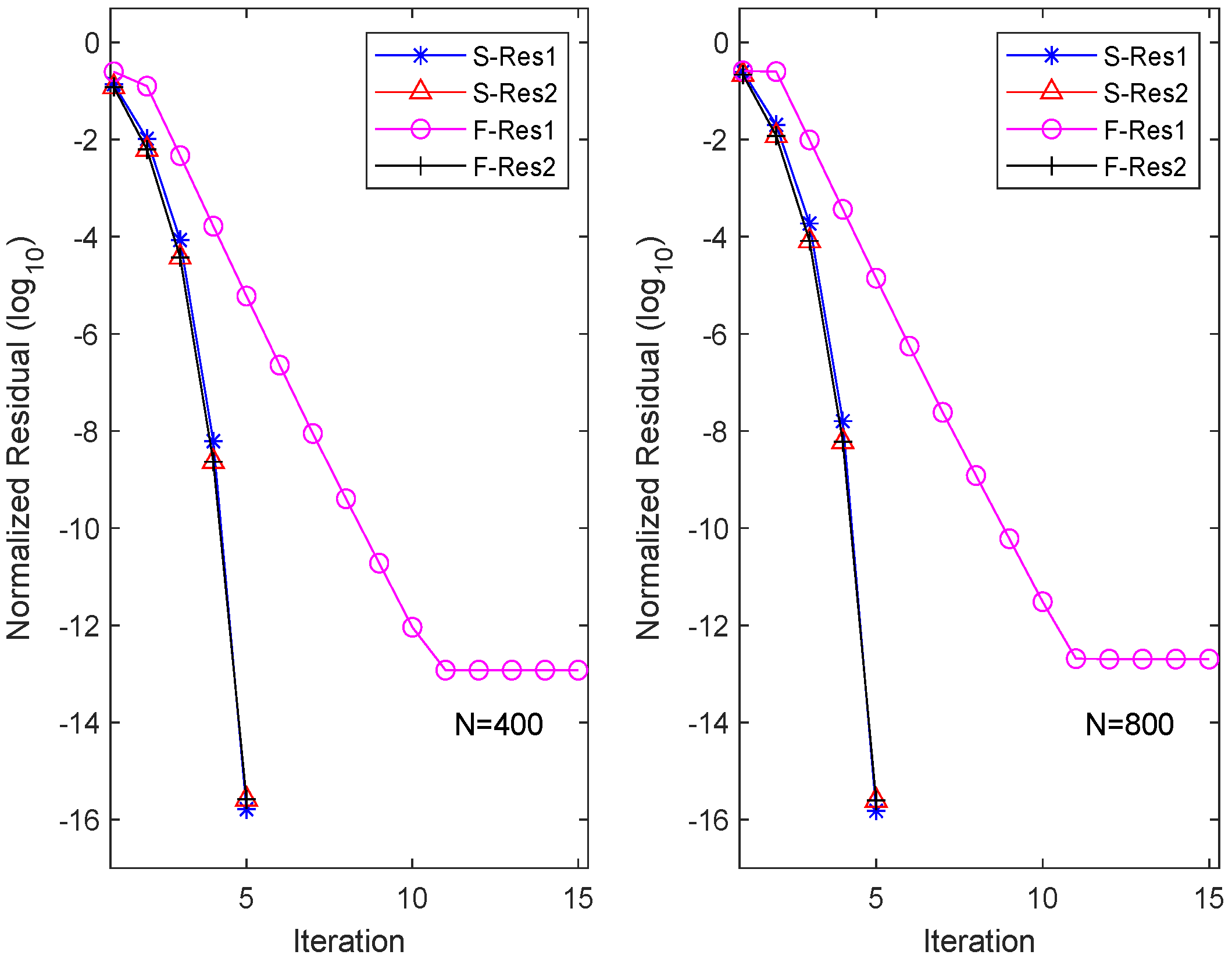
To visualize the residuals of each equation (here, $m=2$) for different iteration methods, we plot the history of the equation residuals in Figure 1. Here, “S-Resi” and “F-Resi” ($i=1,2$) represent the residuals of equations obtained by the OSA and FIX, respectively. The figure illustrates that the OSA has quadratic convergence. Interestingly, although FIX converges rapidly for solving the second equation, it maintains linear convergence for solving the first equation, resulting in an overall linear convergence for FIX.

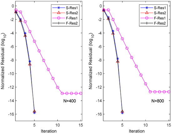
Figure 1. Residual history in each equation for OSA and FIX.

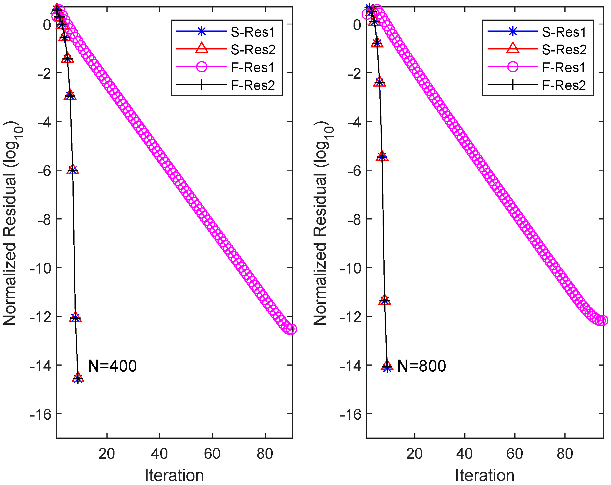
We further consider modified system matrices

$$A_1=0.48\left[{(I+G_1)}^{-1}{\overline{A}}_1\right],A_2=0.98\left[{(I+G_2)}^{-1}{\overline{A}}_2\right],$$

where $G_1$ and $G_2$ are matrices with zero elements except for the last row of $0.6g_1$ and $0.8g_2$, respectively. In this case, the spectral radii of matrices $A_1$ and $A_2$ are 0.96 and 0.95, respectively. We rerun the OSA and FIX algorithm, and the obtained results are recorded in Figure 2. From the plot, it can be observed that for $N=400$, the OSA requires nine iterations to achieve equation residuals at the $O\left({10}^{-15}\right)$ level, with a total time of 10.17 s. Conversely, FIX, after consuming 51.31 s over 90 iterations, only achieves equation residuals at the scale of $O\left({10}^{-13}\right)$. Further numerical experiments demonstrate that even by increasing the number of iterations, FIX fails to further reduce the residual level. Similar numerical results are obtained for the scale of $N=800$.

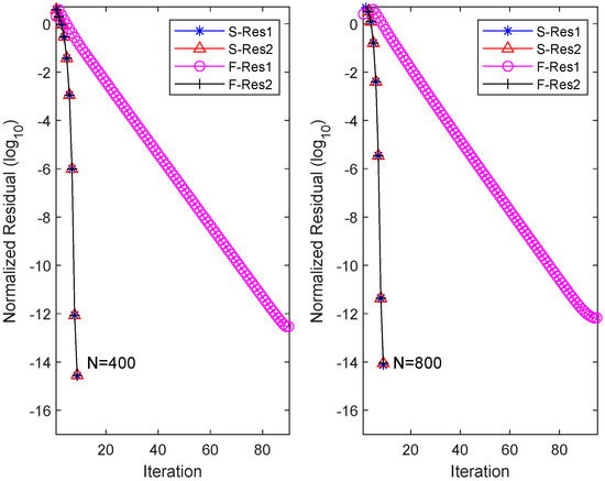
Figure 2. Residual history in each equation for OSA and FIX when $\rho \left(A_1\right)=0.96$ and $\rho \left(A_2\right)=0.95$.

Example 2.

Consider a slight modification of a chemical reaction by a convection reaction partial differential equation on the unit square [27], given by

$$\frac{\partial x}{\partial t}=\frac{{\partial }^{2}x}{\partial y^2}+\frac{{\partial }^{2}x}{\partial z^2}+20\frac{\partial x}{\partial z}-180x+f(y,z)x\left(t\right),$$

where x is a function of time (t), vertical position (v), and horizontal position (z). The boundaries of interest in this problem lie on a square with opposite corners at (0, 0) and (1, 1). The function $x(t,v,z)$ is zero on these boundaries. This PDE is discretized using centered difference approximations on a grid of $n_v\times n_z$ points. The dimension N of A is the product of the state space dimension $n_v{n}_z$, resulting in a sparsity pattern of A as

$$\begin{array}{c}\stackrel{7}{\overbrace{ }}\\ A=\left(\begin{array}{ccccccccc}-734& 171& 0& \cdots & 0& 196& & & \\ -9& -734& \ddots & \ddots & & \ddots & \ddots & & \\ 0& \ddots & \ddots & \ddots & \ddots & & \ddots & \ddots & \\ ⋮& \ddots & \ddots & \ddots & \ddots & \ddots & & \ddots & 196\\ 0& & \ddots & \ddots & \ddots & \ddots & \ddots & & 0\\ 196& \ddots & & \ddots & \ddots & \ddots & \ddots & \ddots & ⋮\\ & \ddots & \ddots & & \ddots & \ddots & \ddots & \ddots & 0\\ & & \ddots & \ddots & & \ddots & \ddots & \ddots & 171\\ & & & 196& 0& \cdots & 0& -9& -734\end{array}\right).\end{array}$$

Here we take

$$A_1={10}^{-3}\times {\xi }_{1}A,A_2={10}^{-3}\times {\xi }_{2}A,Q_1=L_1^Q{\left(L_1^Q\right)}^{\top },Q_2=L_2^Q{\left(L_2^Q\right)}^{\top },$$

where

$$\begin{array}{cc}{\left(L_1^Q\right)}^{\top }=[\stackrel{7}{\overbrace{1,\dots ,1}},0,\dots ,0,\stackrel{7}{\overbrace{1,\dots ,1}}],& {\left(L_2^Q\right)}^{\top }=[\stackrel{7}{\overbrace{0,\dots ,0}},\stackrel{7}{\overbrace{1,\dots ,1}},0,\dots ,0,\stackrel{7}{\overbrace{1,\dots ,1}},\stackrel{7}{\overbrace{0,\dots ,0}}].\end{array}$$

The parameter $m=2$ and the probability matrix $\Pi =\left(\begin{array}{cc}0.244& 0.756\\ 0.342& 0.658\end{array}\right)$.

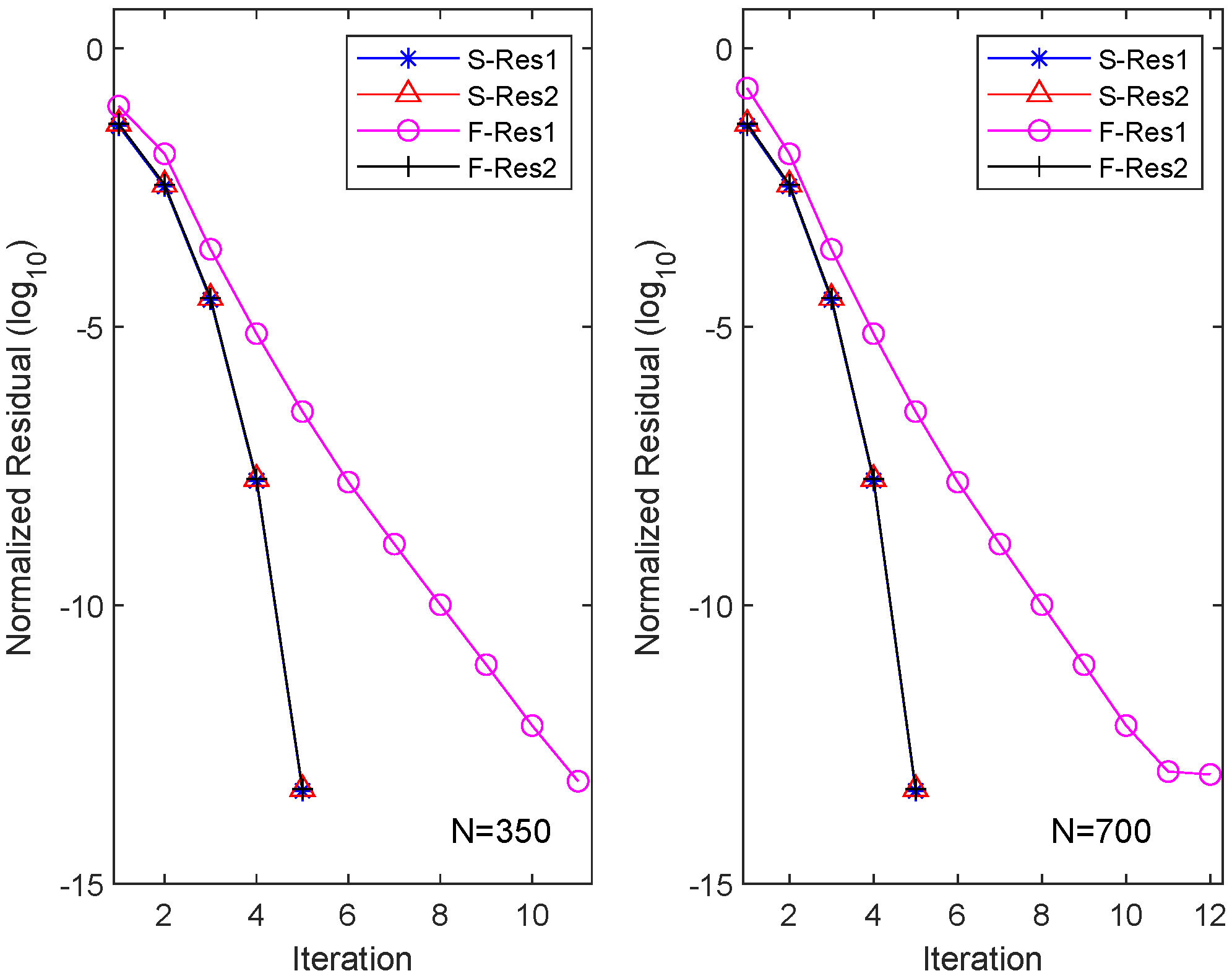
Similarly, we applied the OSA and FIX iterations to CDSEs with dimensions $N=350$ and $N=700$, and the results are presented in Table 2. It is evident that the OSA can achieve equation residuals of $O\left({10}^{-14}\right)$ within five iterations, with the required CPU time approximately one-ninth of that needed for the FIX iterations. However, FIX only attains equation residuals of $O\left({10}^{-13}\right)$ after 10 iterations. We also depict the residuals of the two different iteration methods for their respective m equations (here $m=2$) in Figure 3. The figure illustrates that the OSA exhibits quadratic convergence, while FIX demonstrates only linear convergence.

Table 2. History of CPU time and residual for OSA and FIX in Example 2.

	It.	$\mathit{\delta }{\mathit{t}}_{\mathit{k}}$	${\mathit{t}}_{\mathit{k}}$	Rel_Res	$\mathit{\delta }{\mathit{t}}_{\mathit{k}}$	${\mathit{t}}_{\mathit{k}}$	Rel_Res
			$\mathit{N}=\mathbf{350}$			$\mathit{N}=\mathbf{700}$
	1	$0.001$	$0.001$	$4.37\times {10}^{-2}$	$0.003$	$0.003$	$4.37\times {10}^{-2}$
	2	$0.005$	$0.06$	$3.54\times {10}^{-3}$	$0.003$	$0.006$	$3.54\times {10}^{-3}$
OSA	3	$0.009$	$0.015$	$3.27\times {10}^{-5}$	$0.015$	$0.865$	$3.27\times {10}^{-5}$
	4	$0.032$	$0.047$	$1.85\times {10}^{-8}$	$0.036$	$0.051$	$1.85\times {10}^{-8}$
	5	$0.235$	$0.281$	$5.01\times {10}^{-14}$	$0.331$	$0.382$	$5.01\times {10}^{-14}$
	1	$0.291$	$0.291$	$1.91\times {10}^{-1}$	$1.252$	$1.252$	$1.91\times {10}^{-1}$
	2	$0.231$	$0.523$	$1.27\times {10}^{-2}$	$1.246$	$2.499$	$1.27\times {10}^{-2}$
	3	$0.234$	$0.757$	$2.45\times {10}^{-4}$	$1.294$	$3.793$	$2.45\times {10}^{-4}$
	4	$0.240$	$0.997$	$7.50\times {10}^{-6}$	$1.231$	$5.024$	$7.50\times {10}^{-6}$
	5	$0.227$	$1.224$	$2.99\times {10}^{-7}$	$1.242$	$6.266$	$2.99\times {10}^{-7}$
FIX	6	$0.254$	$1.478$	$1.62\times {10}^{-8}$	$1.215$	$7.482$	$1.62\times {10}^{-8}$
	7	$0.240$	$1.718$	$1.25\times {10}^{-9}$	$1.302$	$8.784$	$1.25\times {10}^{-9}$
	8	$0.228$	$1.946$	$1.02\times {10}^{-10}$	$1.255$	$10.039$	$1.02\times {10}^{-10}$
	9	$0.231$	$2.177$	$8.55\times {10}^{-12}$	$1.243$	$11.281$	$8.55\times {10}^{-12}$
	10	$0.244$	$2.421$	$6.89\times {10}^{-13}$	$1.231$	$12.513$	$6.90\times {10}^{-13}$

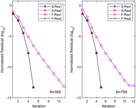
Figure 3. Residual history in each equation for OSA and FIX in Example 2.

3. Structured Algorithm for Large-Scale Problems

In numerous practical scenarios [23], matrix $A_i$ is often sparse, and $Q_i$ is typically of a low-ranked structure. Therefore, in this section, we adapt the OSA to a low-ranked format, well-suited for large-scale computations.

3.1. Structured Iteration Scheme

Given the initial matrices $X_{i,0}=Q_i=L_i^Q{\left(L_i^Q\right)}^{\top }$ for $i=1,\dots ,m$, we show that the iteration (4) can be organized as the following format:

$$\begin{array}{c}{X}_{i,k}=L_{i,k}^Q{K}_{i,k}^Q{\left(L_{i,k}^Q\right)}^{\top },{\mathcal{F}}_{i,k}\left(X_{·,k}\right)=L_{i,k}^{F_{2^k}}{K}_{i,k}^{F_{2^k}}{\left(L_{i,k}^{F_{2^k}}\right)}^{\top },k=0,1,2,\dots ,\hfill \end{array}$$

(7)

where $L_{i,k}^{F_{2^k}}$, $K_{i,k}^{F_{2^k}}$, $L_{i,k}^Q$, and $K_{i,k}^Q$ are of forms in the following proposition.

Proposition 2.

Let $L_i^Q\in {\mathbb{R}}^{N\times l_i}$ in $X_{i,0}$ be the initial factor with $l_i\ll N$. The sequences ${\mathcal{F}}_{i,k}\left(X_{·,k}\right)$ and $X_{i,k}$ generated by (4) are factorized as in (7), where

$$\begin{array}{ccc}& L_{i,k}^{F_{2^k}}=A_i^{\top }[L_{1,k}^{F_{2^k-1}},\dots ,L_{m,k}^{F_{2^k-1}}],K_{i,k}^{F_{2^k}}=p_{i,1}{K}_{1,k}^{F_{2^k-1}}\oplus \dots \oplus p_{i,m}{K}_{m,k}^{F_{2^k-1}},& \hfill \end{array}$$

(8)

$$\begin{array}{cc}& L_{i,k}^Q=[L_{i,k-1}^Q,L_{i,k-1}^{F_{2^k-1}}],K_{i,k}^Q=K_{i,k-1}^Q\oplus K_{i,k-1}^{F_{2^k-1}}\end{array}$$

(9)

and

$$L_{i,k}^{F_1}=A_i^{\top }[L_{1,k}^Q,\dots ,L_{m,k}^Q],K_{i,k}^{F_1}=p_{i,1}{K}_{1,k}^Q\oplus \dots \oplus p_{i,m}{K}_{m,k}^Q,K_{i,0}^Q=I,L_{i,0}^Q=L_i^Q.$$

Proof. 

Given the initial matrix $X_{i,0}=Q_i=L_i^Q{\left(L_i^Q\right)}^{\top }=L_{i,0}^Q{K}_{i,0}^Q{\left(L_{i,0}^Q\right)}^{\top }$, it then follows from (3) that

$${\mathcal{F}}_{i,0}\left(X_{·,0}\right)=A_i^{\top }{E}_i\left(X_{·,0}\right)A_i=A_i^{\top }\left(\sum _{s=1}^m{p}_{i,s}{Q}_s\right)A_i=L_{i,0}^{F_1}{K}_{i,0}^{F_1}{\left(L_{i,0}^{F_1}\right)}^{\top }.$$

So (7) holds for $k=0$. Assume (7) is true for $k=l$. It follows from the iteration scheme (4) that

$$X_{i,l+1}=L_{i,l}^Q{K}_{i,l}^Q{\left(L_{i,l}^Q\right)}^{\top }+L_{i,l}^{F_{2^l}}{K}_{i,l}^{F_{2^l}}{\left(L_{i,l}^{F_{2^l}}\right)}^{\top }=L_{i,l+1}^Q{K}_{i,l+1}^Q{\left(L_{i,l+1}^Q\right)}^{\top }.$$

Recalling (3) again, it follows

$$\begin{array}{ccc}\hfill {\mathcal{F}}_{i,l+1}\left(X_{·,l+1}\right)& =& A_i^{\top }{E}_i\left({\left(A^{\top }E\right)}^{2^{l+1}-1}\left(X_{·,l+1}\right)A^{2^{l+1}-1}\right)A_i\hfill \\ & =& A_i^{\top }{E}_i\left({\left(A^{\top }E\right)}^{2^{l+1}-2}·A^{\top }E\left(X_{·,l+1}\right)A·A^{2^{l+1}-2}\right)A_i\hfill \\ & =& A_i^{\top }{E}_i\left({\left(A^{\top }E\right)}^{2^{l+1}-2}\right(\sum _{s=1}^m{p}_{·,s}{A}_s^{\top }[L_{1,l+1}^Q,\dots ,L_{m,l+1}^Q][p_{s,1}{K}_{1,l+1}^Q\oplus \dots \hfill \\ & & \oplus p_{s,m}{K}_{1,l+1}^Q]{[L_{1,l+1}^Q,\dots ,L_{m,l+1}^Q]}^{\top }{A}_s\left)A^{2^{l+1}-2}\right)A_i\hfill \\ & =& A_i^{\top }{E}_i\left({\left(A^{\top }E\right)}^{2^{l+1}-2}\left(\sum _{s=1}^m{p}_{·,s}{L}_{s,l+1}^{F_1}{K}_{s,l+1}^{F_1}{\left(L_{s,l+1}^{F_1}\right)}^{\top }\right)A^{2^{l+1}-2}\right)A_i\hfill \\ & =& A_i^{\top }{E}_i\left({\left(A^{\top }E\right)}^{2^{l+1}-3}\right(\sum _{s=1}^m{p}_{·,s}{A}_s^{\top }[L_{1,l+1}^{F_1},\dots ,L_{m,l+1}^{F_1}][p_{s,1}{K}_{1,l+1}^{F_1}\oplus \dots \hfill \\ & & \oplus p_{s,m}{K}_{1,l+1}^{F_1}]{[L_{1,l+1}^{F_1},\dots ,L_{m,l+1}^{F_1}]}^{\top }{A}_s\left)A^{2^{l+1}-3}\right)A_i\hfill \\ & =& A_i^{\top }{E}_i\left({\left(A^{\top }E\right)}^{2^{l+1}-3}\left(\sum _{s=1}^m{p}_{·,s}{L}_{s,l+1}^{F_2}{K}_{s,l+1}^{F_2}{\left(L_{s,l+1}^{F_2}\right)}^{\top }\right)A^{2^{l+1}-3}\right)A_i\hfill \\ & =& \dots \hfill \\ & =& A_i^{\top }{E}_i\left(\sum _{s=1}^m{p}_{·,s}{L}_{s,l+1}^{F_{2^{l+1}-1}}{K}_{s,l+1}^{F_{2^{l+1}-1}}{\left(L_{s,l+1}^{F_{2^{l+1}-1}}\right)}^{\top }\right)A_i\hfill \\ & =& L_{i,l+1}^{F_{2^{l+1}}}{K}_{i,l+1}^{F_{2^{l+1}}}{\left(L_{i,l+1}^{F_{2^{l+1}}}\right)}^{\top }.\hfill \end{array}$$

Then (7) holds true for $k=l+1$. The proof is complete. □

3.2. Truncation and Compression

It is evident that the columns of $L_{i,k}^{F_{2^k}}$ at the k-th iteration will scale approximately as $O\left(m^{2^{k-1}}{l}_i\right)$, where $l_i$ is the initial column number of the factor $L_i^Q$. Consequently, we implement the truncation and compression (TC) to reduce the column number of low-rank factors [11,28]. Notably, our algorithm employs the TC technique twice within one iteration: once for $L_{i,k}^{F_{2^k}}$ and once for $L_{i,k}^Q$.

For simplicity in notation, we omit the subscript i for low-rank factors. Recalling (8) and (9), we perform TC on $L_k^{F_{2^k}}$ and $L_k^Q$ using QR decompositions with column pivoting. Then, one has

$$\begin{array}{cc}\hfill & L_k^{F_{2^k}}{P}^{F_{2^k}}=\left[Q^{F_{2^k}}{\tilde{Q}}^{F_{2^k}}\right]\left[\begin{array}{cc}{U}_1^{F_{2^k}}& U_2^{F_{2^k}}\\ 0& {\tilde{U}}^{F_{2^k}}\end{array}\right],\parallel {\tilde{U}}^{F_{2^k}}\parallel <u_0^f\tau ,\\ \hfill & L_k^Q{P}_k^Q=\left[Q_k^Q{\tilde{Q}}_k^Q\right]\left[\begin{array}{cc}{U}_{k,1}^Q& U_{k,2}^Q\\ 0& {\tilde{U}}_k^Q\end{array}\right],\parallel {\tilde{U}}_k^Q\parallel <u_0^q\tau ,\end{array}$$

(10)

where $P^{F_{2^k}}$ and $P_k^Q$ are permutation matrices ensuring that the diagonal elements of the decomposed block triangular matrices decrease in absolute value. Additionally, $u_0^f$ and $u_0^q$ represent constants, and $\tau$ is some small tolerance controlling TC. Let $m^{f_{2^k}}$ and $m_k^q$ denote the respective column numbers of $L_k^{F_{2^k}}$ and $L_k^Q$, bounded above by a given $m_{max}$. Then, their ranks satisfy

$$r^{f_{2^k}}:=\mathrm{rank}\left(L_k^{F_{2^k}}\right)\le m^{f_{2^k}}\le m_{max}\mathrm{and}{r}_k^q:=\mathrm{rank}\left(L_k^Q\right)\le m_k^q\le m_{max}$$

with $m_{max}\ll N$. The truncated factors are still denoted as

$$\begin{array}{cc}& L_k^{F_{2^k}}{P}^{F_{2^k}}=Q^{F_{2^k}}\left[U_1^{F_{2^k}}{U}_2^{F_{2^k}}\right]:=Q^{F_{2^k}}{U}^{F_{2^k}},\end{array}$$

(11)

$$\begin{array}{cc}& L_k^Q{P}_k^Q=Q_k^Q\left[U_{k,1}^Q{U}_{k,2}^Q\right]:=Q_k^Q{U}_k^Q,\end{array}$$

(12)

respectively. The compressed kernels are denoted as

$$\begin{array}{cc}& K_k^{F_{2^k}}:=U^{F_{2^k}}{P}^{F_{2^k}}{K}_k^{F_{2^k}}{\left(U^{F_{2^k}}{P}^{F_{2^k}}\right)}^{\top },\end{array}$$

(13)

$$\begin{array}{cc}& K_k^Q:=U_k^Q{P}_k^Q{K}_k^Q{\left(U_k^Q{P}_k^Q\right)}^{\top },\end{array}$$

(14)

where $K_k^{F_{2^k}}$ and $K_k^Q$ represent the abbreviated kernels in (8) and (9) without subscript i, respectively.

3.3. Computation of Residuals

Given the initial matrix $X_{i,0}=Q_i=L_i^Q{\left(L_i^Q\right)}^{\top }$, for $i=1,\dots ,m$ the initial residual of the CDSEs is

$$\mathcal{S}{c}_0\left(X_{·,0}\right)=X_{i,0}-A_i^{\top }{E}_i\left(X_{·,0}\right)A_i-Q_i=L_{i,0}^R{K}_{i,0}^R{\left(L_{i,0}^R\right)}^{\top },$$

(15)

where $L_{i,0}^R=A_i^{\top }[L_{1,0}^Q,\dots ,L_{m,0}^Q]$, $K_{i,0}^R=p_{i,1}I\oplus ,\dots ,\oplus p_{i,m}I$.

When the k-th iteration $X_{i,k}=L_{i,k}^Q{K}_{i,k}^Q{\left(L_{i,k}^Q\right)}^{\top }$ is available, the residual of CDSEs has the decomposition

$$\mathcal{S}{c}_k\left(X_{·,k}\right)=X_{i,k}-A_i^{\top }{E}_i\left(X_{·,k}\right)A_i-Q_i=L_{i,k}^R{K}_{i,k}^R{\left(L_{i,k}^R\right)}^{\top }$$

(16)

with

$$L_{i,k}^R=[L_{i,0}^Q,L_{i,k}^Q,L_{i,k}^{F_{2^k}}],K_{i,k}^R=-I\oplus K_{i,k}^Q\oplus -K_{i,k}^{F_{2^k}}.$$

Similarly, we also impose the truncation and compression on $L_{i,k}^R,k\ge 0$, i.e, implementing the QR decomposition with pivoting:

$$\begin{array}{cc}\hfill & L_{i,k}^R{P}_{i,k}^R=\left[Q_{i,k}^R{\tilde{Q}}_{i,k}^R\right]\left[\begin{array}{cc}{U}_{i,k,1}^R& U_{i,k,2}^R\\ 0& {\tilde{U}}_{i,k}^R\end{array}\right],\parallel {\tilde{U}}_{i,k}^R\parallel <u_0^r\tau ,\end{array}$$

(17)

where $P_{i,k}^R$ is a pivoting matrix and $u_0^r$ is some constant. Let $U_{i,k}^R=[U_{i,k,1}^R,U_{i,k,2}^R]$. The corresponding kernel of residual is also denoted as

$$\begin{array}{c}\hfill K_{i,k}^R:=U_{i,k}^R{P}_{i,k}^R{K}_{i,k}^R{\left(U_{i,k}^R{P}_{i,k}^R\right)}^{\top },\end{array}$$

(18)

and the terminating condition of the whole algorithm is chosen to be

$$\mathrm{Rel}\_\mathrm{Res}=\underset{i}{max}\frac{\parallel K_{i,k}^R\parallel }{\parallel K_{i,0}^R\parallel }\le ϵ$$

(19)

with $ϵ$ being the tolerance.

3.4. Large-Scale Algorithm and Complexity

The OSA with a low-rank structure equipped with TC is summarized in the following OSA_lr Algorithm 1.

To show the computational complexity of the algorithm OSA_lr, we assume that all matrices $A_i$ for $i=1,\dots ,m$ are sufficiently sparse. This allows us to consider the cost of both the product $A_{i}B$ and solving the equation $A_{i}X=B$, which are both within the range of $cN$ floating-point operations (flops), where B is an $N\times m_b$ matrix with $m_b\ll N$ and c is a constant. Additionally, the number of truncated columns of $L_{i,k}^{F_{2^{k-1}}}$ and $L_{i,k}^Q$ for all $i=1,\dots ,m$ are denoted as $m_k^f$ and $m_k^q$, respectively. The flops and memory of the k-th iteration are summarized in Table 3 below.

Algorithm 1: Algorithm OSA_lr. Solve large-scale CDSEs with low-ranked $Q_i$

Inputs: Sparse matrices $A_i$, low-rank factors $L_i^Q$ for $i=1,\dots ,m$, probability matrix $\Pi \in {\mathbb{R}}^{m\times m}$, truncation tolerance $\tau$, upper bound $m_{max}$ and the iteration tolerance $ϵ$. Outputs: Low-ranked matrix $L_i^X$ and the kernel matrix $K_i^X$ with the solution $X_i\approx L_i^X{K}_i^X{\left(L_i^X\right)}^{\top }$. 1. Set $L_{i,0}^Q=L_i^Q$ and $K_{i,0}^Q=I_i$ for $i=1,\dots ,m$. 2. For $k=1,\dots ,$ until convergence, do 3.  Compute $K_{i,k}^{F_{2^k}}$ and $L_{i,k}^{F_{2^k}}$ as in (8). 4.  Truncate and compress $L_{i,k}^{F_{2^k}}$ as in (10) with accuracy $u_0^f\tau$. 5.  Construct compressed low-ranked factor $L_{i,k}^{F_{2^k}}$ and kernel $K_{i,k}^{F_{2^k}}$ as in (11) and (13). 6.  Compute $K_{i,k}^Q$ and $L_{i,k}^Q$ as in (9). 7.  Truncate and compress $L_{i,k}^q$ as in (10) with accuracy $u_0^q\tau$. 8.  Construct compressed low-ranked factor $L_{i,k}^Q$ and kernel $K_{i,k}^Q$ as in (12) and (14). 9.  Evaluate the relative residual Rel_Res in (19). 11. If Rel_Res $<ϵ$, break, End. 12. $k:=k+1$; 14. End (For) 18. Output $K_i^X:=K_{i,k}^Q$, $L_i^X:=L_{i,k}^Q$.

Table 3. Complexity and memory at k-th iteration in algorithm OSA_lr.

Items	Flops	Memory
$L_{i,k}^{F_{2^{k-1}}}$	$c{m}_{k-1}^q{2}^{k-1}(m^{2^{k-1}}+m)N$	$m^{2^{k-1}}{m}_{k-1}^{q}N$
$K_{i,k}^{F_{2^{k-1}}}$	$m{\left(m_{k-1}^q\right)}^2(1+m^{2k})(k+1)/2$	${\left(m^{2^{k-1}}{m}_{k-1}^q\right)}^2$
$L_{i,k}^{F_{2^{k-1}}}$ QR *	$2{\left(m^{2^{k-1}}{m}_{k-1}^q\right)}^2(N-m^{2^{k-1}}{m}_{k-1}^q/3)$	${\left(m_k^f\right)}^2$
Compressed $K_{i,k}^{F_{2^{k-1}}}$	$4m_k^f{\left(m^{2^{k-1}}{m}_{k-1}^q\right)}^2$	${\left(m_k^f\right)}^2$
$L_{i,k}^Q$	—	$(m_{k-1}^q+m_k^f)N$
$K_{i,k}^Q$	—	${(m_{k-1}^q+m_k^f)}^2$
$L_{i,k}^Q$ QR *	$2{\left(m_k^f{m}_{k-1}^q\right)}^2(N-m_k^f{m}_{k-1}^q/3)$	${\left(m_k^q\right)}^2$
Compressed $K_{i,k}^Q$	$4m_k^q{(m_k^f+m_{k-1}^q)}^2$	${\left(m_k^q\right)}^2$

* Householder QR decomposition is used [29].

3.5. Error Analysis

In this subsection, we will conduct the error analysis of OSA_lr. For $i=1,\dots ,m$, let

$$\delta A_i=A_i-{\widehat{A}}_i,\delta X_{i,k}=X_{i,k}-{\widehat{X}}_{i,k}$$

(20)

be the errors yielded by roundoff or iteration. Here, $A_i$ and $X_{i,k}$ are true matrices, while ${\widehat{A}}_i$ and ${\widehat{X}}_{i,k}$ are the practical iteration matrices. The following lemma indicates the error propagation of the operator.

Lemma 1.

Given errors $\delta X_{i,k}$ and $\delta A_i$ as in (20), the error of the operator is

$$\parallel \delta {\mathcal{F}}_{i,l}\left(X_k\right)\parallel \le {\left(mp\right)}^{2^l}({\alpha }^{2^{l+1}}\delta X_k+2^{l+1}{q}_k{\alpha }^{2^{l+1}-1}\delta A)forl\le k,$$

where $\alpha ={max}_i\{\parallel A_i\parallel \}$, $q_k={max}_i\{\parallel X_{i,k}\parallel \}$, $\delta A={max}_i\{\parallel \delta A_i\parallel \}$, $\delta X_k={max}_i\{\parallel \delta X_{i,k}\parallel \}$, and $p={max}_{i,j}\left\{p_{i,j}\right\}$.

Proof. 

By merely retaining one order error of $\delta A_i$ and $\delta X_{i,k}$, it follows from the definition of ${\mathcal{F}}_{i,l}\left(X_k\right)$ in (3) that the practical operator is

$$\begin{array}{ccc}\hfill {\widehat{\mathcal{F}}}_{i,l}\left(X_k\right)& =& {(A_i+\delta A_i)}^{\top }\stackrel{2^l-1}{\overbrace{\{\sum ^m{p}_{·,·}{(A_j+\delta A_j)}^{\top }\cdots \{\sum ^m{p}_{·,·}{(A_s+\delta A_s)}^{\top }}}\left[\sum ^m{p}_{·,·}(X_{·,k}+\delta X_{·,k})\right]·\hfill \\ & & \stackrel{2^l-1}{\overbrace{(A_s+\delta A_s)\}\cdots (A_j+\delta A_j)\}}}(A_i+\delta A_i)\hfill \\ & \le & {(A_i+\delta A_i)}^{\top }\stackrel{2^l-2}{\overbrace{\{\sum ^m{p}_{·,·}{(A_j+\delta A_j)}^{\top }\cdots \{\sum ^m{p}_{·,·}{(A_t+\delta A_t)}^{\top }}}[{\mathcal{F}}_{i,0}\left(X_k\right)+{\left(mp\right)}^2(A_s^{\top }\delta X_{·,k}{A}_s\hfill \\ & & +{\left(\delta A_s\right)}^{\top }{X}_{·,k}{A}_s+A_s^{\top }{X}_{·,k}\delta A_s\left)\right]\stackrel{2^l-2}{\overbrace{(A_t+\delta A_t)\}\cdots (A_j+\delta A_j)\}}}(A_i+\delta A_i)\hfill \\ & \le & {(A_i+\delta A_i)}^{\top }\stackrel{2^l-3}{\overbrace{\{\sum ^m{p}_{·,·}{(A_j+\delta A_j)}^{\top }\cdots \{\sum ^m{p}_{·,·}{(A_u+\delta A_u)}^{\top }}}[{\mathcal{F}}_{i,1}\left(X_k\right)+{\left(mp\right)}^3({\left(A_s{A}_t\right)}^{\top }\delta X_{·,k}{A}_s{A}_t\hfill \\ & & +{\left(\delta A_s{A}_t\right)}^{\top }{X}_{·,k}{A}_s{A}_t+{\left(A_s{A}_t\right)}^{\top }{X}_{·,k}\delta A_s{A}_t+{\left(A_s\delta A_t\right)}^{\top }{X}_{·,k}{A}_s{A}_t\hfill \end{array}$$

(21)

$$\begin{array}{ccc}& & +{\left(\delta A_s{A}_t\right)}^{\top }{X}_{·,k}{A}_s{A}_t\left)\right]\stackrel{2^l-3}{\overbrace{(A_u+\delta A_u)\}\cdots (A_j+\delta A_j)\}}}(A_i+\delta A_i)\hfill \\ & \le & \cdots \hfill \end{array}$$

(22)

Note that error items in $\left[·\right]$ in (21) and (22) have corresponding upper bounds ${\left(mp\right)}^2({\alpha }^2\delta X_k+2q_k\alpha \delta A)$ and ${\left(mp\right)}^3({\alpha }^4\delta X_k+4q_k{\alpha }^3\delta A)$, respectively. After multiplying the left by ${(A_i+\delta A_i)}^{\top }$ and the right by $A_i+\delta A_i$ in the outermost layer, the upper bounds of the errors are ${\left(mp\right)}^2({\alpha }^4\delta X_k+4q_k{\alpha }^3\delta A)$ and ${\left(mp\right)}^3({\alpha }^6\delta X_k+6q_k{\alpha }^5\delta A)$, respectively. Then, by the induction, it is not difficult to see that the final error is

$${\left(mp\right)}^{2^l}({\alpha }^{2^{l+1}}\delta X_k+2^{l+1}{q}_k{\alpha }^{2^{l+1}-1}\delta A).$$

 □

We have the following error bound at the $k+1$-th iteration.

Theorem 2.

Given errors $\delta X_k$ and $\delta A_i$ as in (20), the error at the $k+1$-th iteration has the bound

$$\delta X_{k+1}\le {(1+\left(mp{\alpha }^2\right))}^{2^k}\delta X_k+2^{k+1}{\left(mp\right)}^{2^k}{\alpha }^{2^{k+1}-1}{q}_k\delta A+O\left(\tau \right),$$

(23)

where m, p, α, and $q_k$ are defined in Lemma 1 and τ is the error of TC described in Section 3.2.

Proof. 

It follows from the iteration format (4) that the error at the $k+1$-th iteration has the upper bound

$$\parallel \delta X_{i,k+1}\parallel \le \parallel \delta X_{i,k}\parallel +\parallel \delta {\mathcal{F}}_{i,k}\left(X_k\right)\parallel +O\left(\tau \right),$$

where $O\left(\tau \right)$ represents the truncation and compression error on ${\mathcal{F}}_{i,k}\left(X_k\right)$ and $X_{i,k}$. By taking $l=k$ in Lemma 1, one has

$$\parallel \delta X_{i,k+1}\parallel \le \delta X_k+{\left(mp\right)}^{2^k}{\alpha }^{2^k+1}\delta X_k+2^{k+1}{\left(mp\right)}^{2^k}{q}_k{\alpha }^{2^{k+1}-1}\delta A+O\left(\tau \right)$$

and (23) holds true. □

4. Numerical Examples

In this section, we illustrate the effectiveness of OSA_lr in computing symmetric solutions to large-scale CDSEs (1) through practical examples [23,26,27,30,31,32,33]. The algorithm OSA_lr was coded by MATLAB 2019a on a 64-bit PC running Windows 10. The computer is equipped with a 3.0 GHz Intel Core i5 processor with six cores and six threads, 32 GB RAM, and a machine unit roundoff value of eps = $2.22\times {10}^{-16}$. The maximum allowed column number of the low-ranked factors in OSA_lr is bounded by $m_{max}$ = 1000, and the tolerance for the TC of columns is set to $\tau ={10}^{-16}$. In our experiments, we also attempted using $N·$eps as the TC tolerance for $\tau$ but found it had no impact on the computation accuracy. The residuals of the equations are calculated in (19) with a termination tolerance of $ϵ={10}^{-13}$. It is noteworthy that we no longer compare with the linearly convergent iterative methods in Section 2, as the computational complexity of those algorithms per iteration is $O\left(N^3\right)$.

Example 3.

We still employ the modification of the all-pass SISO system [26] in Section 2, but here we take N = 12,000. We list the calculated results of OSA_lr in Table 4, where the columns ${\delta }_k$ and $t_k$ record the CPU time for each iteration and for cumulative iterations, respectively. The Resi and Rel_Resi ($i=1,2$) columns provide the absolute residual $\parallel K_{i,k}^R\parallel$ and relative residual $\parallel K_{i,k}^R\parallel /\parallel K_{i,0}^R\parallel$ computed by OSA_lr at each iteration, respectively. The $m_k^{Q_i}$ ($i=1,2$) columns indicate the column number of the low-ranked factor $L_{i,k}^Q$.

Table 4. CPU time and residual in Example 3.

It.	$\mathit{\delta }{\mathit{t}}_{\mathit{k}}$	${\mathit{t}}_{\mathit{k}}$	Res1	Rel_Res1	Res2	Rel_Res2	${\mathit{m}}_{\mathit{k}}^{{\mathit{Q}}_1}$	${\mathit{m}}_{\mathit{k}}^{{\mathit{Q}}_2}$
1	$0.012$	$0.012$	$2.06\times {10}^0$	$2.06\times {10}^0$	$3.06\times {10}^0$	$3.06\times {10}^0$	3	3
2	$0.135$	$0.147$	$1.35\times {10}^{-1}$	$1.35\times {10}^{-1}$	$6.15\times {10}^{-2}$	$6.15\times {10}^{-2}$	9	9
3	$0.659$	$0.806$	$1.44\times {10}^{-3}$	$1.44\times {10}^{-3}$	$6.44\times {10}^{-4}$	$6.44\times {10}^{-4}$	21	21
4	$35.765$	$35.571$	$1.80\times {10}^{-7}$	$1.80\times {10}^{-7}$	$7.51\times {10}^{-8}$	$7.51\times {10}^{-8}$	46	46
5	$488.519$	$525.090$	$4.42\times {10}^{-14}$	$4.42\times {10}^{-14}$	$2.72\times {10}^{-14}$	$2.72\times {10}^{-14}$	109	109

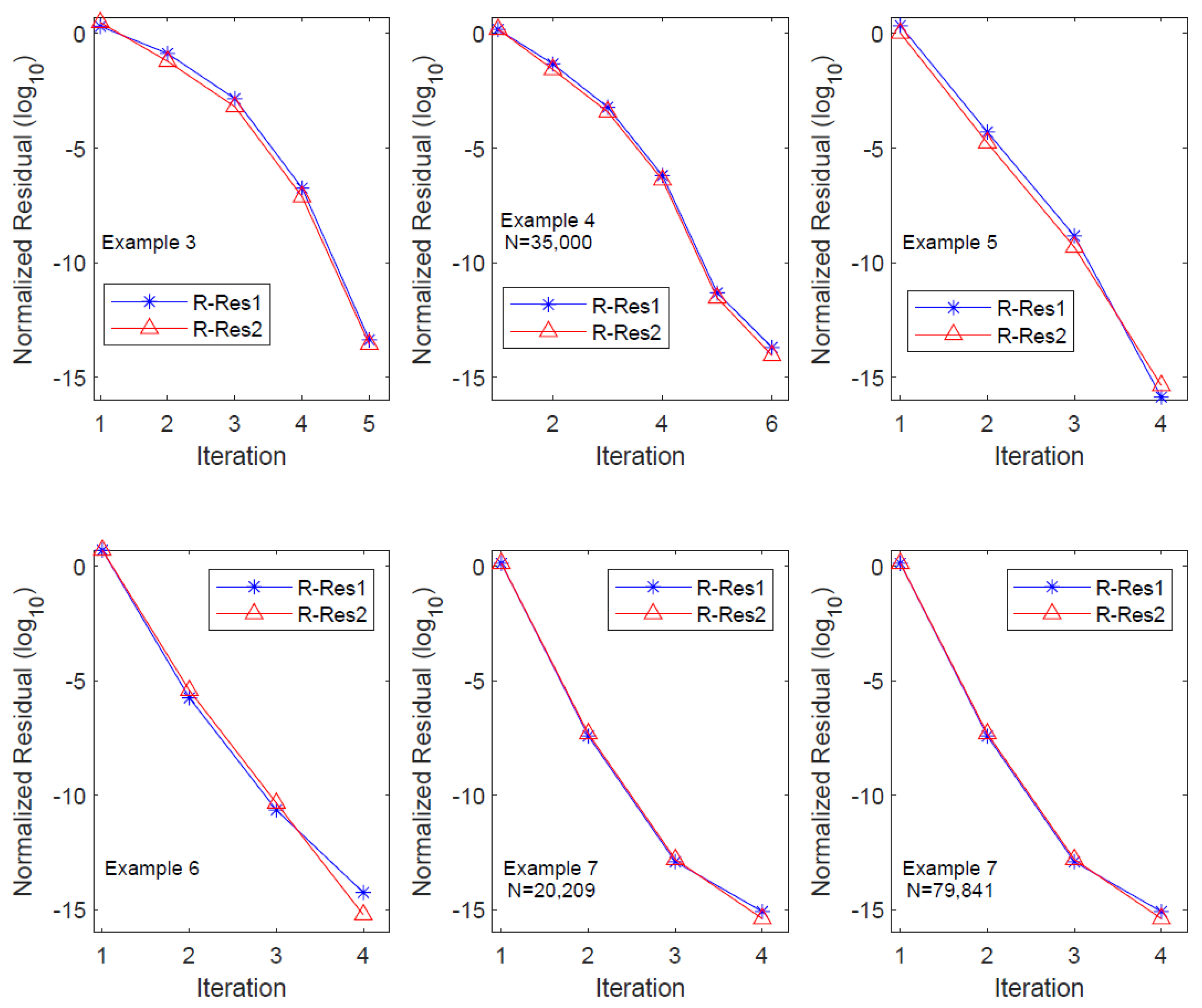
From the table, it is evident that OSA_lr achieves the prescribed equation residual level within five iterations, and the residual history demonstrates the quadratic convergence of the algorithm. The column count $m_k^{Q_i}$ for the low-ranked factor $L_{i,k}^Q$ expands at a rate greater than twice with each iteration, resulting in an exponential increase in the CPU time. Particularly, significant growth in the CPU time occurs during the third and fourth iterations. In numerical experiments, we observed that this substantial increase in the CPU time primarily lies in the residual computation step, specifically in Step 9 of OSA_lr. Hence, further investigation on the efficient evaluation of the equation residual is a crucial consideration for large-scale computations. We also plot the residual history of OSA_lr in Figure 7 to show its performance, where R-Res_i ($i=1,2$) denotes the relative residual of the i-th equation.

Example 4.

We continue to examine CDSEs from Example 2 [27,30], but with larger scales N = 21,000, 28,000, and 35,000. The derived results of OSA_lr are presented in Table 5.

Table 5. CPU time and residual in Example 4.

It.	$\mathit{\delta }{\mathit{t}}_{\mathit{k}}$	${\mathit{t}}_{\mathit{k}}$	Res1	Rel_Res1	Res2	Rel_Res2	${\mathit{m}}_{\mathit{k}}^{{\mathit{Q}}_1}$	${\mathit{m}}_{\mathit{k}}^{{\mathit{Q}}_2}$
				N = 21,000
1	$0.005$	$0.005$	$1.51\times {10}^1$	$1.51\times {10}^1$	$1.55\times {10}^1$	$1.55\times {10}^1$	3	3
2	$0.010$	$0.015$	$4.73\times {10}^{-2}$	$4.73\times {10}^{-2}$	$2.70\times {10}^{-2}$	$2.70\times {10}^{-2}$	7	7
3	$0.019$	$0.034$	$6.10\times {10}^{-4}$	$6.10\times {10}^{-4}$	$3.83\times {10}^{-4}$	$3.83\times {10}^{-4}$	15	15
4	$0.053$	$0.088$	$6.30\times {10}^{-7}$	$6.30\times {10}^{-7}$	$4.04\times {10}^{-7}$	$4.04\times {10}^{-7}$	31	31
5	$1.354$	$1.441$	$3.67\times {10}^{-12}$	$3.67\times {10}^{-12}$	$2.37\times {10}^{-12}$	$2.37\times {10}^{-12}$	157	157
6	$235.119$	$235.119$	$1.93\times {10}^{-14}$	$1.93\times {10}^{-14}$	$7.13\times {10}^{-15}$	$7.13\times {10}^{-15}$	908	908
				N = 28,000
1	$0.006$	$0.006$	$1.51\times {10}^1$	$1.51\times {10}^1$	$1.55\times {10}^1$	$1.55\times {10}^1$	3	3
2	$0.017$	$0.023$	$4.73\times {10}^{-2}$	$4.73\times {10}^{-2}$	$2.70\times {10}^{-2}$	$2.70\times {10}^{-2}$	7	7
3	$0.029$	$0.052$	$6.10\times {10}^{-4}$	$6.10\times {10}^{-4}$	$3.83\times {10}^{-4}$	$3.83\times {10}^{-4}$	15	15
4	$0.078$	$0.130$	$6.30\times {10}^{-7}$	$6.30\times {10}^{-7}$	$4.04\times {10}^{-7}$	$4.04\times {10}^{-7}$	31	31
5	$1.373$	$1.503$	$4.09\times {10}^{-12}$	$4.09\times {10}^{-12}$	$2.86\times {10}^{-12}$	$2.86\times {10}^{-12}$	147	147
6	$239.690$	$241.193$	$1.59\times {10}^{-14}$	$1.59\times {10}^{-14}$	$8.68\times {10}^{-15}$	$8.68\times {10}^{-15}$	908	908
				N = 35,000
1	$0.008$	$0.008$	$1.51\times {10}^1$	$1.51\times {10}^1$	$1.55\times {10}^1$	$1.55\times {10}^1$	3	3
2	$0.025$	$0.034$	$4.73\times {10}^{-2}$	$4.73\times {10}^{-2}$	$2.70\times {10}^{-2}$	$2.70\times {10}^{-2}$	7	7
3	$0.043$	$0.077$	$6.10\times {10}^{-4}$	$6.10\times {10}^{-4}$	$3.83\times {10}^{-4}$	$3.83\times {10}^{-4}$	15	15
4	$0.098$	$0.175$	$6.30\times {10}^{-7}$	$6.30\times {10}^{-7}$	$4.04\times {10}^{-7}$	$4.04\times {10}^{-7}$	31	31
5	$1.617$	$1.793$	$4.76\times {10}^{-12}$	$4.76\times {10}^{-12}$	$3.46.\times {10}^{-12}$	$3.46\times {10}^{-12}$	161	161
6	$248.356$	$250.148$	$1.97\times {10}^{-14}$	$1.97\times {10}^{-14}$	$8.62\times {10}^{-15}$	$8.62\times {10}^{-15}$	908	908

The symbols ${\delta }_k$, $t_k$, Resi, Rel_Resi, and $m_k^{Q_i}$ ($i=1,2$) are defined similarly to those in Example 3. In all experiments, the equation residuals (in $log10$) reached the predetermined residual level by the sixth iteration. For equations of different dimensions, the Resi $(i=1,2)$ columns indicate that the algorithm OSA_lr is of nearly quadratic convergence, except for the final two iterations. The $m_k^{Q_i}$ column reveals that, in the fifth and sixth iterations, the column number of the factor $L_{i,k}^Q$ increased by nearly five times and six times, respectively. This resulted in a substantial increase in the CPU time during the last two iterations. A further detailed analysis indicated that this increased time primarily came from the computation of equation residuals in the final two steps. The performance of OSA_lr on the residual history with N = 35,000 is plotted in Figure 7, where R-Res_i ($i=1,2$) denotes the relative residual of the i-th equation.

Example 5.

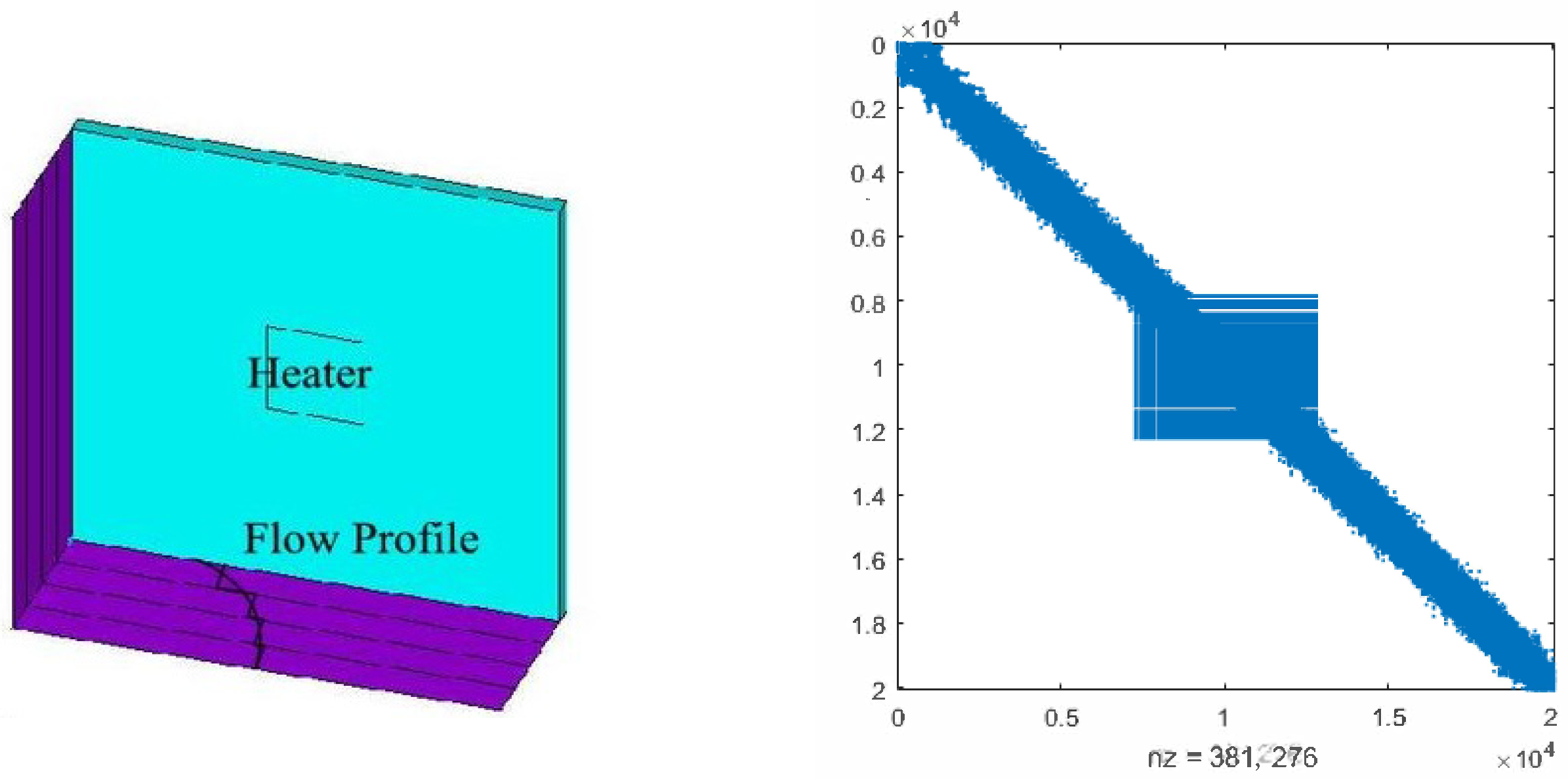
Consider the thermal convective flow control systems in [23,30,31]. These problems involve a flow region with a prescribed velocity profile, incorporating convective transport. Achieving solution accuracy with upwind finite element schemes typically requires a considerable number of elements for a physically meaningful simulation. In the illustrated scenario (see the left side of Figure 4), a 3D model of a chip is subjected to forced convection, utilizing tetrahedral element type SOLID70 as described by [34]. Both the Dirichlet boundary conditions and initial conditions are set to 0.

Figure 4. The 3D model of the chip and the discretized matrix $A_1$.

We consider the case that the fluid speed is zero and the discretization matrices are symmetric. The system matrices are

$$A_1={(I+r_{1}B{B}^{\top })}^{-1}A,A_2={(I+r_{2}B{B}^{\top })}^{-1}A,Q_1=Q_2=C^{\top }C,$$

where $r_1$ and $r_2$ are random numbers from (0, 1) and matrices $A\in {\mathrm{R}}^{N\times N}$, $B\in {\mathrm{R}}^{N\times 1}$, and $C\in {\mathrm{R}}^{1\times N}$ (N = 20,082) can be found at [23]. Since $A_1$ and $A_1$ have almost the same sparse structure, we only plot $A_1$ in the right of Figure 4, where the non-zero elements attain the scale of 381,276. In the numerical experiments, we set $m=2$ and use the probability matrix $\Pi =\left(\begin{array}{cc}0.631& 0.369\\ 0.143& 0.857\end{array}\right)$. We ran OSA_lr for 10 different $r_1$ and $r_2$ and recorded the averaged CPU time, residual of CDSEs, and column dimension of the low-ranked factor in Table 6.

Table 6. CPU time and residual in Example 5.

It.	$\mathit{\delta }{\mathit{t}}_{\mathit{k}}$	${\mathit{t}}_{\mathit{k}}$	Res1	Rel_Res1	Res2	Rel_Res2	${\mathit{m}}_{\mathit{k}}^{{\mathit{Q}}_1}$	${\mathit{m}}_{\mathit{k}}^{{\mathit{Q}}_2}$
1	$0.017$	$0.017$	$2.06\times {10}^{-1}$	$2.22\times {10}^0$	$6.13\times {10}^{-1}$	$1.05\times {10}^0$	10	10
2	$0.083$	$0.100$	$9.73\times {10}^{-6}$	$5.03\times {10}^{-5}$	$9.83\times {10}^{-6}$	$1.69\times {10}^{-5}$	22	22
3	$0.665$	$0.766$	$2.74\times {10}^{-10}$	$1.47\times {10}^{-9}$	$2.75\times {10}^{-10}$	$4.72\times {10}^{-10}$	46	46
4	$1073.56$	$1074.34$	$2.48\times {10}^{-17}$	$1.33\times {10}^{-16}$	$2.49\times {10}^{-16}$	$4.28\times {10}^{-16}$	112	112

The computational results in Table 6 reveal that OSA_lr requires only four iterations to achieve the predetermined equation residual accuracy. Moreover, the Resi and Rel_Resi columns indicate that OSA_lr exhibits quadratic convergence. The $m_k^{Q_i}$ column demonstrates that the column count of the low-rank factor $L_k^{Q_i}$ approximately doubles in the first three iterations but experiences a close to three-fold increase in the final iteration. In terms of the CPU time for each iteration, the time required for the final iteration is significantly greater than the sum of the preceding three. A detailed analysis indicates that the primary reason for this phenomenon is similar to the previous examples, wherein the computation of equation residuals in the algorithm accounts for the majority of the time. The performance of OSA_lr on the residual history is plotted in Figure 7, where R-Res_i ($i=1,2$) denotes the relative residual of the i-th equation.

Example 6.

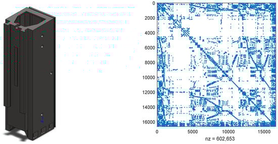
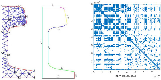
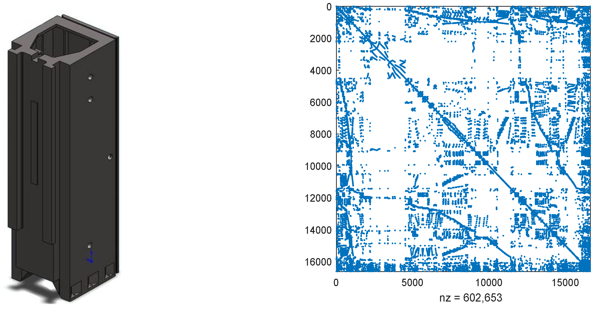
Consider the structurally vertical stand model from machinery control systems, depicted on the left side of Figure 5, representing a segment of a machine tool [30]. In this structural component, a set of guide rails is situated on one of its surfaces. Throughout the machining process, a tool slide traverses various positions along these rails [32]. The model was created and meshed using ANSYS. For spatial discretization, the finite element method with linear Lagrange elements was employed and implemented in FEniCS.

Figure 5. The vertical stand model and the discretized matrix $A_1$.

The derived system matrices are

$$\begin{array}{cc}{A}_1=-0.01\left[{(I+r_{1}B{B}^{\top })}^{-1}A\right],& A_2=-0.015\left[{(I+r_{2}B{B}^{\top })}^{-1}A\right],\\ Q_1=L_1^Q{\left(L_1^Q\right)}^{\top },& Q_2=L_2^Q{\left(L_2^Q\right)}^{\top },\end{array}$$

where $r_1$ and $r_2$ are random numbers from (0, 1) and $L_1^Q$ and $L_2^Q\in {\mathrm{R}}^{N\times 1}$ are vectors with all elements being zeros except fives ones located in rows (3341, 6743, 8932, 11,324, and 16,563) and rows (1046, 2436, 6467, 8423, and 12,574), respectively. As the sparse structures of $A_1$ and $A_2$ are analogous, the right of Figure 5 only exhibits the structure of $A_1$, which contains 602,653 non-zero elements. Matrices $A\in {\mathrm{R}}^{16,626\times 16,626}$ and $B\in {\mathrm{R}}^{16,626\times 1}$ can be found at [23]. In this example, we set $m=2$ and use the probability matrix as $\Pi =\left(\begin{array}{cc}0.564& 0.436\\ 0.785& 0.215\end{array}\right)$.

We utilized OSA_lr to solve the CDSEs, and the computed results are presented in Table 7. It can be observed from the table that OSA_lr terminates after four iterations, achieving a high-precision solution, where the equation residuals reach a level of $O\left({10}^{-15}\right)$ to $O\left({10}^{-16}\right)$. The iteration history in the Resi and Rel_Resi columns illustrates the quadratic convergence of OSA_lr. The $m_k^{Q_i}$ column indicates that in the second, third, and fourth iterations, the column count of the low-rank factor $L_k^{Q_i}$ approximately doubles, triples, and quadruples, respectively. This demonstrates that the truncation and compression techniques have a limited impact on reducing the column count of $L_k^{Q_i}$ in this scenario. Similarly, $\delta t_k$ reveals that the CPU time for the final iteration is significantly greater than the sum of the preceding three, primarily due to the algorithm spending substantial time computing equation residuals in the last iteration.

Table 7. CPU time and residual in Example 6.

It.	$\mathit{\delta }{\mathit{t}}_{\mathit{k}}$	${\mathit{t}}_{\mathit{k}}$	Res1	Rel_Res1	Res2	Rel_Res2	${\mathit{m}}_{\mathit{k}}^{{\mathit{Q}}_1}$	${\mathit{m}}_{\mathit{k}}^{{\mathit{Q}}_2}$
1	$0.023$	$0.023$	$5.01\times {10}^0$	$5.01\times {10}^0$	$5.01\times {10}^0$	$5.01\times {10}^0$	3	3
2	$0.091$	$0.114$	$1.78\times {10}^{-6}$	$1.78\times {10}^{-6}$	$3.77\times {10}^{-6}$	$3.77\times {10}^{-6}$	7	7
3	$0.787$	$0.901$	$2.25\times {10}^{-10}$	$2.25\times {10}^{-11}$	$4.52\times {10}^{-11}$	$4.52\times {10}^{-11}$	25	25
4	$164.941$	$165.842$	$5.59\times {10}^{-15}$	$5.59\times {10}^{-15}$	$5.96\times {10}^{-16}$	$5.96\times {10}^{-16}$	119	119

Example 7.

Consider a semi-discretized heat transfer problem aimed at optimizing the cooling of steel profiles in control systems, as discussed in works by [23,30]. The order of the models varies due to the application of different refinements to the computational mesh. For the discretization process, the ALBERTA-1.2 fem-toolbox [33] and the linear Lagrange elements are utilized. The initial mesh (depicted on the left in Figure 6) is generated using MATLAB’s pdetool.

Figure 6. The initial mesh for cooling of steel and the discretized matrix $A_1$ and $A_2$.

We slightly modify the model matrices as follows:

$$\begin{array}{cc}{A}_1=r_1\left[{(I+B{B}^{\top })}^{-1}A\right],& A_2=r_2\left[{(I+B{B}^{\top })}^{-1}A\right],\\ Q_1=L_1^Q{\left(L_1^Q\right)}^{\top },& Q_2=L_2^Q{\left(L_2^Q\right)}^{\top },\end{array}$$

where $r_1=0.009$ and $r_2=0.008$ for N = 20,209 and $r_1=0.0015$ and $r_2=0.0012$ for N = 79,841. In this experiment, we take $L_1^Q=r_3{C}^{\prime }$ and $L_2^Q=r_4{C}^{\prime }$, with $r_3$, $r_4$ being a random number in (0, 1). Matrices $A\in {\mathrm{R}}^{N\times N}$, $B\in {\mathrm{R}}^{N\times 1}$, and $C\in {\mathrm{R}}^{1\times N}$ can be found at [23]. The sparse structures of matrices $A_1$ and $A_2$ are nearly identical, and for illustration purposes, we only display the structure of $A_1$ with N = 79,841 on the right side of Figure 6. The probability matrix is defined as

$$\Pi =\left(\begin{array}{cc}0.713& 0.287\\ 0.584& 0.416\end{array}\right).$$

We employed OSA_lr to solve CDSEs under two different dimensions, and the computed results are presented in Table 8. It is evident from the table that OSA_lr terminates after achieving the predetermined equation residual levels for various dimensions. The Rel_Resi column indicates a significant decrease in the relative equation residuals to the level of $O\left({10}^{-8}\right)$ by the second iteration, enabling the algorithm to obtain a high-precision solution in only four iterations. The two columns of $m_k^{Q_i}$ demonstrate that, for different dimensions, the column count of the low-rank factor $L_k^{Q_i}$ increases by a factor of two, indicating that truncation and compression techniques effectively constrain the growth of the column count of $L_k^{Q_i}$ in this scenario. Similarly, the $\delta t_k$ column reveals that in the final iteration, due to the computation of equation residuals, OSA_lr consumes considerably more CPU time than the sum of the preceding three iterations. The performances of OSA_lr on the residual history with N = 20,209, 799,841 are plotted in Figure 7, where R-Res_i ($i=1,2$) denotes the relative residual of the i-th equation.

Table 8. CPU time and residual in Example 7.

It.	$\mathit{\delta }{\mathit{t}}_{\mathit{k}}$	${\mathit{t}}_{\mathit{k}}$	Res1	Rel_Res1	Res2	Rel_Res2	${\mathit{m}}_{\mathit{k}}^{{\mathit{Q}}_1}$	${\mathit{m}}_{\mathit{k}}^{{\mathit{Q}}_2}$
				N = 20,209
1	$0.011$	$0.011$	$8.30\times {10}^0$	$1.34\times {10}^0$	$6.82\times {10}^0$	$1.34\times {10}^0$	12	12
2	$0.052$	$0.063$	$2.39\times {10}^{-7}$	$3.84\times {10}^{-8}$	$2.48\times {10}^{-7}$	$4.86\times {10}^{-8}$	24	24
3	$0.129$	$0.192$	$7.72\times {10}^{-13}$	$1.24\times {10}^{-13}$	$8.01\times {10}^{-11}$	$1.57\times {10}^{-13}$	48	48
4	$489.420$	$489.612$	$5.13\times {10}^{-15}$	$8.25\times {10}^{-16}$	$2.07\times {10}^{-15}$	$4.06\times {10}^{-16}$	96	96
				N = 79,841
1	$0.614$	$0.614$	$8.29\times {10}^0$	$1.33\times {10}^0$	$6.81\times {10}^0$	$1.33\times {10}^0$	12	12
2	$5.140$	$5.754$	$1,77\times {10}^{-7}$	$2.84\times {10}^{-8}$	$1.06\times {10}^{-7}$	$2.09\times {10}^{-8}$	24	24
3	$16.946$	$22.700$	$4.74\times {10}^{-12}$	$7.63\times {10}^{-13}$	$2.86\times {10}^{-12}$	$5.60\times {10}^{-13}$	48	48
4	$874.870$	$895.570$	$2.73\times {10}^{-15}$	$4.39\times {10}^{-16}$	$3.67\times {10}^{-15}$	$7.19\times {10}^{-16}$	96	96

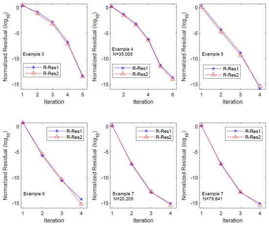
Figure 7. Relative residual histories for OSA_lr in Examples 3–7.

5. Conclusions

This paper introduces an OSA method for coupled Stein equations in a class of jump systems. The convergence of the algorithm is established. For large-structured problems, the OSA method is extended to a low-rank structured iterative format, and an error propagation analysis of the algorithm is conducted. Numerical experiments, drawn from practical problems [23], indicate that in small-scale computations, the OSA outperforms existing linearly convergent iterative methods in terms of both the CPU time and accuracy. In large-scale computations, OSA_lr efficiently computes high-precision solutions for CDSEs. Nevertheless, the experiments reveal that the time spent on residual computation in the final iteration is relatively high. Therefore, improving the efficiency of the algorithm’s termination criteria is a direction for further research in future work, and it is currently under consideration.

References

- Chen, C.-T. Linear System Theory and Design, 3rd ed.; Oxford University Press: New York, NY, USA, 1999. [Google Scholar]
- Betser, A.; Cohen, N.; Zeheb, E. On solving the Lyapunov and Stein equations for a companion matrix. Syst. Control Lett. 1995, 25, 211–218. [Google Scholar] [CrossRef]
- Hueso, J.L.; Martínez, G.; Hernández, V. A systolic algorithm for the triangular Stein equation. J. VLSI Signal Process. Syst. Signal Image Video Technol. 1993, 5, 49–55. [Google Scholar] [CrossRef]
- Li, T.-X.; Weng, P.C.-Y.; Chu, E.K.-W.; Lin, W.-W. Large-scale Stein and Lyapunov Equations, Smith Method, and Applications. Numer. Algorithms 2013, 63, 727–752. [Google Scholar] [CrossRef]
- Fan, H.-Y.; Weng, P.C.-Y.; Chu, K.-W. Numerical solution to generalized Lyapunov/Stein and rational Riccati equations in stochastic control. Numer. Algorithms 2016, 71, 245–272. [Google Scholar] [CrossRef]
- Yu, B.; Dong, N.; Tang, Q. Factorized squared Smith method for large-scale Stein equations with high-rank terms. Automatica 2023, 154, 111057. [Google Scholar] [CrossRef]
- Borno, I.; Gajic, Z. Parallel algorithm for solving coupled algebraic Lyapunov equations of discrete-time jump linear systems. Comput. Math. Appl. 1995, 30, 1–4. [Google Scholar] [CrossRef]
- Wu, A.-G.; Duan, G.-R. New Iterative algorithms for solving coupled Markovian jump Lyapunov equations. IEEE Trans. Auto. Control 2015, 60, 289–294. [Google Scholar]
- Zhou, B.; Duan, G.-R.; Li, Z.-Y. Gradient based iterative algorithm for solving coupled matrix equations. Syst. Control. Lett. 2009, 58, 327–333. [Google Scholar] [CrossRef]
- Li, Z.-Y.; Zhou, B.; Lam, J.; Wang, Y. Positive operator based iterative algorithms for solving Lyapunov equations for Itô stochastic systems with Markovian jumps. Appl. Math. Comput. 2011, 217, 8179–8195. [Google Scholar] [CrossRef]
- Yu, B.; Fan, H.-Y.; Chu, E.K.-W. Smith method for projected Lyapunov and Stein equations. UPB Sci. Bull. Ser. A 2018, 80, 191–204. [Google Scholar]
- Sun, H.-J.; Zhang, Y.; Fu, Y.-M. Accelerated smith iterative algorithms for coupled Lyapunov matrix equations. J. Frankl. Inst. 2017, 354, 6877–6893. [Google Scholar] [CrossRef]
- Li, T.-Y.; Gajic, Z. Lyapunov iterations for solving coupled algebraic Riccati equations of Nash differential games and algebraic Riccati equations of zero-sum games. In New Trends in Dynamic Games and Applications; Olsder, G.J., Ed.; Annals of the International Society of Dynamic Games; Birkhäuser: Boston, MA, USA, 1995; Volume 3. [Google Scholar]
- Wicks, M.; De Carlo, R. Solution of Coupled Lyapunov Equations for the Stabilization of Multimodal Linear Systems. In Proceedings of the 1997 American Control Conference (Cat. No.97CH36041), Albuquerque, NM, USA, 4–6 June 1997; Volume 3, pp. 1709–1713. [Google Scholar]
- Ivanov, I.G. An Improved method for solving a system of discrete-time generalized Riccati equations. J. Numer. Math. Stoch. 2011, 3, 57–70. [Google Scholar]
- Qian, Y.-Y.; Pang, W.-J. An implicit sequential algorithm for solving coupled Lyapunov equations of continuous-time Markovian jump systems. Automatica 2015, 60, 245–250. [Google Scholar] [CrossRef]
- Costa, O.L.V.; Aya, J.C.C. Temporal difference methods for the maximal solution of discrete-time coupled algebraic Riccati equations. J. Optim. Theory Appl. 2001, 109, 289–309. [Google Scholar] [CrossRef]
- Costa, O.L.V.; Marques, R.P. Maximal and stabilizing Hermitian solutions for discrete-time coupled algebraic Riccati equations. Math. Control Signals Syst. 1999, 12, 167–195. [Google Scholar] [CrossRef]
- Ivanov, I.G. Stein iterations for the coupled discrete-time Riccati equations. Nonlinear Anal. Theory Methods Appl. 2009, 71, 6244–6253. [Google Scholar] [CrossRef]
- Bai, L.; Zhang, S.; Wang, S.; Wang, K. Improved SOR iterative method for coupled Lyapunov matrix equations. Afr. Math. 2021, 32, 1457–1463. [Google Scholar] [CrossRef]
- Tian, Z.-L.; Xu, T.-Y. An SOR-type algorithm based on IO iteration for solving coupled discrete Markovian jump Lyapunov equations. Filomat 2021, 35, 3781–3799. [Google Scholar] [CrossRef]
- Penzl, T. A cyclic low-rank Smith method for large sparse Lyapunov equations. SIAM J. Sci. Comput. 1999, 21, 1401–1408. [Google Scholar] [CrossRef]
- Korvink, G.; Rudnyi, B. Oberwolfach Benchmark Collection. In Dimension Reduction of Large-Scale Systems; Benner, P., Sorensen, D.C., Mehrmann, V., Eds.; Lecture Notes in Computational Science and Engineering; Springer: Berlin/Heidelberg, Germany, 2005; Volume 45. [Google Scholar]
- Wang, Q.; Lam, J.; Wei, Y.; Chen, T. Iterative solutions of coupled discrete Markovian jump Lyapunov equations. Comput. Math. Appl. 2008, 55, 843–850. [Google Scholar] [CrossRef]
- Mathworks. MATLAB User’s Guide; Mathworks: Natick, MA, USA, 2020; Available online: https://www.mathworks.com/help/pdf_doc/matlab/index.html (accessed on 15 March 2024).
- Ober, R.J. Asymptotically Stable All-Pass Transfer Functions: Canonical Form, Parametrization and Realization. IFAC Proc. Vol. 1987, 20, 181–185. [Google Scholar] [CrossRef]
- Chahlaoui, Y.; Van Dooren, P. Benchmark examples for model reduction of linear time-invariant dynamical systems. In Dimension Reduction of Large-Scale Systems; Springer: Berlin/Heidelberg, Germany, 2005; Volume 45, pp. 379–392. [Google Scholar]
- Chu, E.K.-W.; Weng, P.C.-Y. Large-scale discrete-time algebraic Riccati equations—Doubling algorithm and error analysis. J. Comput. Appl. Math. 2015, 277, 115–126. [Google Scholar] [CrossRef]
- Higham, N.J. Functions of Matrices: Theory and Computation; SIAM: Philadelphia, PA, USA, 2008. [Google Scholar]
- Chahlaoui, Y.; Van Dooren, P. A collection of benchmark examples for model reduction of linear time invariant dynamical systems. Work. Note 2002. Available online: https://eprints.maths.manchester.ac.uk/1040/1/ChahlaouiV02a.pdf (accessed on 15 March 2024).
- Moosmann, C.; Greiner, A. Convective thermal flow problems. In Dimension Reduction of Large-Scale Systems; Lecture Notes in Computational Science and Engineering; Springer: Berlin/Heidelberg, Germany, 2005; Volume 45, pp. 341–343. [Google Scholar]
- Lang, N. Numerical Methods for Large-Scale Linear Time-Varying Control Systems and Related Differential Matrix Equations; Logos-Verlag: Berlin, Germany, 2018. [Google Scholar]
- Schmidt, A.; Siebert, K. Design of Adaptive Finite Element Software—The Finite Element Toolbox ALBERTA; Lecture Notes in Computational Science and Engineering; Springer: Berlin/Heidelberg, Germany, 2005; Volume 42. [Google Scholar]
- Harper, C.A. Electronic Packaging and Interconnection Handbook; McGraw-Hill: New York, NY, USA, 1997. [Google Scholar]
Disclaimer/Publisher’s Note: The statements, opinions and data contained in all publications are solely those of the individual author(s) and contributor(s) and not of MDPI and/or the editor(s). MDPI and/or the editor(s) disclaim responsibility for any injury to people or property resulting from any ideas, methods, instructions or products referred to in the content. |
© 2024 by the authors. Licensee MDPI, Basel, Switzerland. This article is an open access article distributed under the terms and conditions of the Creative Commons Attribution (CC BY) license (https://creativecommons.org/licenses/by/4.0/).