Developing Higher-Order Unconditionally Positive Finite Difference Methods for the Advection Diffusion Reaction Equations

Abstract

This study introduces the higher-order unconditionally positive finite difference (HUPFD) methods to solve the linear, nonlinear, and system of advection–diffusion–reaction (ADR) equations. The stability and consistency of the developed methods are analyzed, which are necessary and sufficient for the numerical approach to converge to the exact solution. The problem under consideration is of the Cauchy type, and hence, Von Neumann stability analysis is used to analyze the stability of the proposed schemes. The HUPFD’s efficacy and efficiency are investigated by calculating the error, convergence rate, and computing time. For validation purposes, the higher-order unconditionally positive finite difference solutions are compared to analytical calculations. The numerical results demonstrate that the proposed methods produce accurate solutions to solve the advection diffusion reaction equations. The results also show that increasing the order of the unconditionally positive finite difference leads an implicit scheme that is conditionally stable and has a higher order of accuracy with respect to time and space.

1. Introduction

The advection–diffusion–reaction (ADR) equation is important in the application of various physical and chemical processes, such as absorption of pollutants in soil, exponential travelling waves, modeling of semiconductors, and modeling of biological processes, among others [1,2,3]. The ADR equation is a partial differential equation generally represented by the equation below:

$$\begin{array}{cc}\hfill & {\displaystyle \frac{\partial u}{\partial t}}+U_a{\displaystyle \frac{\partial u}{\partial x}}-D{\displaystyle \frac{{\partial }^{2}u}{\partial x^2}}=f(t,x,u),(x,t)\in [a,b]\times [0,T]t>0,\hfill \\ \hfill & u(0,x)=u_0\left(x\right)\ge 0,\hfill \\ \hfill & u(a,t)=u_a\left(t\right)u(b,t)=u_b\left(t\right).\hfill \end{array}$$

(1)

where D is the diffusion coefficient, $U_a$ represent the advection coefficient, $u_x(t,x)$ is the advection term, $u_{xx}(t,x)$ is the diffusion term, $u_t(t,x)$ is the rate at which the concentration of substances changes over time, and $f(t,x,u)$ is the reaction term or the source [4]. The advection–diffusion–reaction equation governs the process of advection and diffusion simultaneously [5,6,7,8].

In this paper, we develop the higher-order unconditionally positive finite difference methods (HUPFD) and apply them to solve the ADR equations. These methods extends to the unconditionally positive finite difference method (UPFD) developed by Chen-Charpentier and Kojouharov [1] and it has subsequently been utilized by several other researchers, such as [9,10,11]. The primary advantage of the UPFD is that it guarantees the positivity of solutions regardless of time step or mesh size. Numerical techniques that preserve solution positivity are crucial in physical applications, in quantities such as chemical species concentration, population sizes, and neutron numbers [1] wherein only positive solution have meaning. The ADR equations are often difficult to solve exactly, and hence, the need to develop numerical methods that are good in solving the problem as accurately as possible with less computational time. Benito M et al. studied an unconditionally positivity-preserving scheme for solving the ADR equation. In this study, they found the UPFD schme produces good results when solving the ADR equation as compared to Crank–Nicolson method, and also that the method works for a larger time steps [1]. Appadu A.R. studied the unconditionally positive schemes for biofilm formation on medical implant using the Allen–Cahn equation. In this study, he found that the proposed method produced good results, and that it is stable at all times for all step sizes $h,k>0$ [9]. Mahamond et al. tested and improved a nonconventional UPFD method, in which they found that the UPFD scheme is convergent time integrator with order 1, which necessitates investigation of the higher-order UPFD scheme [12]. The study of higher-order numerical methods is of keen interest in the field of fluid dynamics, mathematical physics, engineering, etc, because they are known to produce highly accurate solutions [13,14]. Much research effort is put into developing efficient numerical methods that converge to the solution quickly and with less computational time [15,16,17].

The novel HUPFD schemes we developed are validated on the linear, nonlinear, and system of ADR equations, and its findings are compared with those obtained using the exact solution, UPFD, Crank–Nicolson, and nonstandard finite difference methods. The efficiency of the developed approaches is assessed by comparing the errors, convergence rates, and computing times. In recent years, there has been significant interest in higher-order finite difference approaches. Kovac et al. (2021) introduced a novel approach for solving the diffusion or heat equation using explicit numerical methods. These approaches incorporate Huxley and Fisher’s reaction terms, which proved analytically that the convergence of the approaches for linear ordinary differential systems occurs at a fourth order in the time step size. Additionally, it was found that the provided methods are applicable to solve nonlinear equations in stiff cases. Kovacs et al. (2024) developed a novel two-stage explicit approach for the solution of partial differential equations that involve a diffusion and two reaction terms. A large system with random characteristics and discontinuous initial condition was utilized in this investigation. The researchers demonstrated that in the linear cases, the accuracy of the approaches follows a second order of accuracy, and it is unconditionally stable. Gurarslan et al. (2013) introduced a sixth-order compact difference scheme and a fourth-order Runge–Kutta scheme to generate numerical solutions for the one-dimensional advection–diffusion equation. In this study, the solutions were found to be highly accurate in solving the concurrent transport equation for the one-dimensional advection–diffusion equation. Other examples can be found in [18,19,20,21,22,23,24,25,26,27,28,29,30,31,32,33]. The need for the development of HUPFD approaches arise from the limitations observed in numerical methods. In order to achieve accuracy in solutions for solving majority of the partial differential equations, a significant amount of computational time is required.

This study primarily focuses on the development and evaluation of the HUPFD, showing that augmenting the order of the UPFD schemes to higher-order results in an implicit scheme that is unconditionally stable, and progressively improves its accuracy with respect to time and space.

The subsequent sections of the paper are structured sequentially. Section 2 provides an introduction to the UPFD, Section 3 focuses on the development of the HUPFD, and Section 4 and Section 5 include the numerical analysis of the linear advection–diffusion–reaction equation using the HUPFD, which include stability analysis and consistency of the methods. The efficiency and effectiveness of the HUPFD approach in solving the linear advection–diffusion–reaction equations has been shown by numerical examples in Section 6. These examples are presented in comparison to the analytical results. The conclusion of the investigation is presented in Section 7.

2. The Unconditionally Positive Finite Difference Scheme

In this section, we present details of the UPFD schemes [1] as given below:

$${\displaystyle \frac{\partial u}{\partial x}}\approx \{\begin{array}{cc}\frac{u_i^n-u_{i-1}^{n+1}}{\Delta x}& \hfill \mathrm{(2a)}\\ \frac{u_i^{n+1}-u_{i-1}^n}{\Delta x}& \hfill \mathrm{(2b)}\end{array}$$

$$\begin{array}{cc}\hfill {\displaystyle \frac{\partial u}{\partial t}}& \approx {\displaystyle \frac{u_i^{n+1}-u_i^n}{\Delta t}}\hfill \end{array}$$

(3)

$$\begin{array}{cc}\hfill {\displaystyle \frac{{\partial }^{2}u}{\partial x^2}}& \approx {\displaystyle \frac{u_{i+1}^n-2u_i^{n+1}+u_{i-1}^n}{{(\Delta x)}^2}}\hfill \end{array}$$

(4)

where the spatial step size is $\Delta x={\displaystyle \frac{b-a}{m-1}}$ and the grid points are given as $x_i=a+\Delta x(i-1)$, $1\le i\le m$. The time step size $\Delta t={\displaystyle \frac{T}{N-1}}$, with the corresponding grid points given as $t_n=\Delta t(n-1)$, $1\le n\le N$.

Note that when approximating the derivatives of the first and second space, the terms in the finite difference schemes are evaluated at different time levels n and $n+1$. This is required to preserve the positivity of the solution. Equation (2a) is used when the coefficient of the first space derivative is negative, while Equation (2b) is used when the derivative is positive. Conversely, Equation (4) is employed regardless of the positive or negative nature of the coefficient of the second space derivative. However, when the negative coefficient to the diffusion term is used, the solution is expected to blow up, which will undoubtedly impact stability.

3. Development of the Higher-Order Unconditionally Positive Finite Difference Schemes

The development of the higher-order unconditionally positive finite difference (HUPFD) involves the study of three distinct cases, resulting in the formulation of three different algorithms, denoted as HUPFD 1, HUPFD 2, and HUPFD 3. The objective is to develop a robust approach, based on the principles of the UPFD, which preserves the positivity of solutions. The process of developing finite difference schemes for space derivatives in practical situations involves a careful consideration of the tradeoffs between accuracy, stability, consistency, and computing costs. Engineers and scientists employ varying methods in accordance with the specific demands of their simulations and the limitations imposed by their computational resources, with a primary focus on attaining accuracy. This study focuses on the construction of HUPFD schemes utilizing various orders within finite difference schemes for space derivative schemes. The objective is to explore combinations that yield improved results. The unconditionally positive finite difference methods are a category of methods used to approximate the solution of partial differential equations. These methods are applicable to various real-life problems, including heat transfer, stress/strain mechanics, fluid dynamics, and electromagnetics.

3.1. HUPFD 1

In this case, the higher-order method is achieved by considering the first-order formula for the first space derivative and the fourth-order approximation for the second space derivative, as shown below:

$${\displaystyle \frac{\partial u}{\partial x}}\approx \{\begin{array}{cc}\frac{u_i^n-u_{i-1}^{n+1}}{\Delta x}& \hfill \mathrm{(5a)}\\ \frac{u_i^{n+1}-u_{i-1}^n}{\Delta x}& \hfill \mathrm{(5b)}\end{array}$$

$$\begin{array}{cc}\hfill {\displaystyle \frac{\partial u}{\partial t}}& \approx {\displaystyle \frac{u_i^{n+1}-u_i^n}{\Delta t}}\hfill \end{array}$$

(6)

$$\begin{array}{cc}\hfill {\displaystyle \frac{{\partial }^{2}u}{\partial x^2}}& \approx {\displaystyle \frac{-u_{i+2}^{n+1}+16u_{i+1}^n-30u_i^{n+1}+16u_{i-1}^n-u_{i-2}^{n+1}}{12\Delta x^2}}\hfill \end{array}$$

(7)

where the spatial step size is $\Delta x={\displaystyle \frac{b-a}{m-1}}$ and the grid points are given as $x_i=a+\Delta x(i-1)$, $2\le i\le m-1$.

3.2. HUPFD 2

In this case, the HUPFD scheme is obtained by considering the second-order formula for the first space derivative and the fourth-order formula for the second space derivative, as shown below:

$${\displaystyle \frac{\partial u}{\partial x}}\approx \{\begin{array}{cc}\frac{u_{i+1}^{n+1}-u_{i-1}^n}{2\Delta x}& \hfill \mathrm{(8a)}\\ \frac{u_{i+1}^n-u_{i-1}^{n+1}}{2\Delta x}& \hfill \mathrm{(8b)}\end{array}$$

$$\begin{array}{cc}\hfill {\displaystyle \frac{\partial u}{\partial t}}& \approx {\displaystyle \frac{u_i^{n+1}-u_i^n}{\Delta t}},\hfill \end{array}$$

(9)

$$\begin{array}{cc}\hfill {\displaystyle \frac{{\partial }^{2}u}{\partial x^2}}& \approx {\displaystyle \frac{-u_{i+2}^{n+1}+16u_{i+1}^n-30u_i^{n+1}+16u_{i-1}^n-u_{i-2}^{n+1}}{12\Delta x^2}}.\hfill \end{array}$$

(10)

where the spatial step size is $\Delta x={\displaystyle \frac{b-a}{m-1}}$ and the grid points are given as $x_i=a+\Delta x(i-1)$, $2\le i\le m-1$.

3.3. HUPFD 3

In this case, HUPFD schemes are obtained by considering the fourth-order formula for the derivatives of the first and second space, as shown below:

$${\displaystyle \frac{\partial u}{\partial x}}\approx \{\begin{array}{cc}\frac{-u_{i+2}^n+8u_{i+1}^{n+1}-8u_{i-1}^n+u_{i-2}^{n+1}}{12\Delta x}& \hfill \mathrm{(11a)}\\ \frac{-u_{i+2}^{n+1}+8u_{i+1}^n-8u_{i-1}^{n+1}+u_{i-2}^n}{12\Delta x}& \hfill \mathrm{(11b)}\end{array}$$

$$\begin{array}{cc}\hfill {\displaystyle \frac{\partial u}{\partial t}}& \approx {\displaystyle \frac{u_i^{n+1}-u_i^n}{\Delta t}}\hfill \end{array}$$

(12)

$$\begin{array}{cc}\hfill {\displaystyle \frac{{\partial }^{2}u}{\partial x^2}}& \approx {\displaystyle \frac{-u_{i+2}^{n+1}+16u_{i+1}^n-30u_i^{n+1}+16u_{i-1}^n-u_{i-2}^{n+1}}{12\Delta x^2}}\hfill \end{array}$$

(13)

where the spatial step size is $\Delta x={\displaystyle \frac{b-a}{m-1}}$ and the grid points are given as $x_{i-1}=a+\Delta x(i-2)$, $2\le i\le m-1$.

4. Implementation of the Higher-Order Unconditionally Positive Finite Difference Schemes on the Linear ADR Equation

In this section, we set $f(t,x,u)=-u$, $U_a=1$, and $D=1$ in Equation (1) to obtain the equation given below:

$$\begin{array}{c}\hfill {\displaystyle \frac{\partial u}{\partial t}}+{\displaystyle \frac{\partial u}{\partial x}}={\displaystyle \frac{{\partial }^{2}u}{\partial x^2}}-u,\end{array}$$

(14)

subject to the following initial and boundary conditions:

$$\begin{array}{c}\hfill \left\{\begin{array}{c}u(x,0)=e^{-x},0\le x\le 10\hfill \\ u(0,t)=e^t,0\le t\le 0.85\hfill \\ u_x(10,t)=-u(10,t),0\le t\le 0.85\hfill \end{array}\right.\end{array}$$

(15)

with the exact solution given by $u(x,t)=e^{(t-x)}$ [1].

4.1. Solving the Linear ADR Equation Using the HUPFD 1 Scheme

Since the coefficient of ${\displaystyle \frac{\partial u}{\partial x}}$ in Equation (14) is positive, we use Equations (5b)–(7) to find the UPFD scheme. Therefore, the HUPFD discretization of Equation (14) is given by the equation below:

$$\begin{array}{c}\hfill {\displaystyle \frac{u_i^{n+1}-u_i^n}{\Delta t}}+{\displaystyle \frac{u_i^{n+1}-u_{i-1}^n}{\Delta x}}={\displaystyle \frac{-u_{i+2}^{n+1}+16u_{i+1}^n-30u_i^{n+1}+16u_{i-1}^n-u_{i-2}^{n+1}}{12\Delta x^2}}-u_i^{n+1},\end{array}$$

(16)

which simplifies to the following:

$$\begin{array}{cc}\hfill {\displaystyle \frac{1}{12\Delta x^2}}{u}_{i-2}^{n+1}& +\left({\displaystyle \frac{1}{\Delta t}}+{\displaystyle \frac{1}{\Delta x}}+{\displaystyle \frac{30}{12\Delta x^2}}+1\right)u_i^{n+1}\hfill \\ \hfill & +{\displaystyle \frac{1}{12\Delta x^2}}{u}_{i+2}^{n+1}={\displaystyle \frac{1}{\Delta t}}{u}_i^n+\left({\displaystyle \frac{1}{\Delta x}}+{\displaystyle \frac{16}{12D{x}^2}}\right)u_{i-1}^2+{\displaystyle \frac{16}{12\Delta x^2}}{u}_{i+1}^n.\hfill \end{array}$$

(17)

Let $p_1={\displaystyle \frac{1}{\Delta t}}+{\displaystyle \frac{1}{\Delta x}}+{\displaystyle \frac{30}{12\Delta x^2}}+1$, $p_2={\displaystyle \frac{1}{12\Delta x^2}}$,$p_3={\displaystyle \frac{1}{2\Delta t}}$, $p_4={\displaystyle \frac{1}{\Delta x}}+{\displaystyle \frac{16}{12\Delta x^2}}$, thus

$$\begin{array}{c}\hfill p_1{u}_i^{n+1}+p_2{u}_{i+2}^{n+1}+p_2{u}_{i-2}^{n+1}=p_3{u}_i^n+p_4{u}_{i-1}^n+16p_2{u}_{i+1}^n.\end{array}$$

(18)

Equation (18) is simplified to the following:

$$\begin{array}{c}\hfill A{u}^{n+1}=B{u}^n+d^n,\end{array}$$

(19)

where:

$$\begin{array}{c}\hfill A{u}^{n+1}=\left[\begin{array}{ccccccc}{p}_1& 0& p_2& 0& 0& \cdots & 0\\ 0& p_1& 0& p_2& 0& \cdots & ⋮\\ p_2& 0& p_1& 0& p_2& \ddots & ⋮\\ 0& p_2& 0& p_1& 0& \ddots & 0\\ 0& 0& p_2& 0& p_1& \ddots & p_2\\ ⋮& \ddots & \ddots & \ddots & \ddots & \ddots & 0\\ 0& \cdots & \cdots & \cdots & p_2& 0& p_1\end{array}\right]\left[\begin{array}{c}{u}_1^{n+1}\\ u_2^{n+1}\\ u_3^{n+1}\\ ⋮\\ ⋮\\ ⋮\\ u_{m-1}^{n+1}\\ u_m^{n+1}\end{array}\right]\end{array}$$

(20)

$$\begin{array}{c}\hfill B{u}^n=\left[\begin{array}{ccccccc}{p}_3& 16p_2& 0& 0& 0& \cdots & 0\\ p_4& p_3& 16p_2& 0& 0& \cdots & ⋮\\ 0& p_4& p_3& 16p_2& 0& \ddots & ⋮\\ 0& 0& p_4& p_3& 16p_2& \ddots & 0\\ 0& 0& 0& p_4& p_3& \ddots & 0\\ ⋮& \ddots & \ddots & \ddots & \ddots & \ddots & 16p_2\\ 0& \cdots & \cdots & \cdots & 0& p_4& p_3\end{array}\right]\left[\begin{array}{c}{u}_1^n\\ u_2^n\\ u_3^n\\ ⋮\\ ⋮\\ ⋮\\ u_{m-1}^n\\ u_m^n\end{array}\right]\end{array}$$

(21)

and:

$$\begin{array}{c}\hfill d^n=p_3\left[\begin{array}{c}{u}_0^n\\ 0\\ 0\\ ·\\ ·\\ ·\\ ·\\ ·\\ ·\\ ·\\ ·\\ u_m^n\end{array}\right]-p_2\left[\begin{array}{c}{u}_0^{n+1}\\ 0\\ 0\\ ·\\ ·\\ ·\\ ·\\ ·\\ ·\\ ·\\ ·\\ u_{m+1}^{n+1}\end{array}\right]\end{array}$$

(22)

where u is the unknown vector of the order $m\times 1$ at any time level $t^{n+1}$ and A and B are the coefficient square matrix of order $m\times m$ with a triangular structure.

4.1.1. Consistency

We investigate the consistency by using the Taylor expansion on the point $(i,n)$. The Taylor expansions of $u_i^{n+1},u_i^{n-1},u_{i-1}^n,u_{i+1}^n,u_{i-2}^{n+1},u_{i+2}^{n+1}$ are as follows:

$$\begin{array}{cc}\hfill u_i^{n+1}& \approx u_i^n+\Delta t{\displaystyle \frac{\partial u}{\partial t}}+{\displaystyle \frac{{(\Delta t)}^2}{2}}{\displaystyle \frac{{\partial }^{2}u}{\partial t^2}}+{\displaystyle \frac{{(\Delta t)}^3}{6}}{\displaystyle \frac{{\partial }^{3}u}{\partial t^3}}+\cdots \hfill \\ \hfill u_i^{n-1}& \approx u_i^n-\Delta t{\displaystyle \frac{\partial u}{\partial t}}+{\displaystyle \frac{{(\Delta t)}^2}{2}}{\displaystyle \frac{{\partial }^{2}u}{\partial t^2}}-{\displaystyle \frac{{(\Delta t)}^3}{6}}{\displaystyle \frac{{\partial }^{3}u}{\partial t^3}}+\cdots \hfill \\ \hfill u_{i-1}^n& \approx u_i^n-\Delta x{\displaystyle \frac{\partial u}{\partial x}}+{\displaystyle \frac{{(\Delta x)}^2}{2}}{\displaystyle \frac{{\partial }^{2}u}{\partial x^2}}-{\displaystyle \frac{{(\Delta x)}^3}{6}}{\displaystyle \frac{{\partial }^{3}u}{\partial x^3}}+\cdots \hfill \\ \hfill u_{i+1}^n& \approx u_i^n+\Delta x{\displaystyle \frac{\partial u}{\partial x}}+{\displaystyle \frac{{(\Delta x)}^2}{2}}{\displaystyle \frac{{\partial }^{2}u}{\partial x^2}}+{\displaystyle \frac{{(\Delta x)}^3}{6}}{\displaystyle \frac{{\partial }^{3}u}{\partial x^3}}+\cdots \hfill \\ \hfill u_{i-2}^{n+1}& \approx u_i^n+\Delta t{\displaystyle \frac{\partial u}{\partial t}}-2\Delta x{\displaystyle \frac{\partial u}{\partial x}}+2{(\Delta x)}^2{\displaystyle \frac{{\partial }^{2}u}{\partial x^2}}-2(\Delta t\Delta x){\displaystyle \frac{{\partial }^{2}u}{\partial t\partial x}}+{\displaystyle \frac{{(\Delta t)}^2}{2}}{\displaystyle \frac{{\partial }^{2}u}{\partial t^2}}+\cdots \hfill \\ \hfill u_{i+2}^{n+1}& \approx u_i^n+\Delta t{\displaystyle \frac{\partial u}{\partial t}}+2\Delta x{\displaystyle \frac{\partial u}{\partial x}}+2{(\Delta x)}^2{\displaystyle \frac{{\partial }^{2}u}{\partial x^2}}+2(\Delta t\Delta x){\displaystyle \frac{{\partial }^{2}u}{\partial t\partial x}}+{\displaystyle \frac{{(\Delta t)}^2}{2}}{\displaystyle \frac{{\partial }^{2}u}{\partial t^2}}+\cdots \hfill \end{array}$$

(23)

By substituting Equation (23) into (18), we obtain the following:

$$\begin{array}{cc}\hfill & p_2\left(u_i^n+\Delta t{\displaystyle \frac{\partial u}{\partial t}}-2\Delta x{\displaystyle \frac{\partial u}{\partial x}}+2{(\Delta x)}^2{\displaystyle \frac{{\partial }^{2}u}{\partial x^2}}-2(\Delta t\Delta x){\displaystyle \frac{{\partial }^{2}u}{\partial t\partial x}}+{\displaystyle \frac{{(\Delta t)}^2}{2}}{\displaystyle \frac{{\partial }^{2}u}{\partial t^2}}+\cdots \right)\hfill \\ \hfill & +p_1\left(u_i^n+\Delta t{\displaystyle \frac{\partial u}{\partial t}}+{\displaystyle \frac{{(\Delta t)}^2}{2}}{\displaystyle \frac{{\partial }^{2}u}{\partial t^2}}+{\displaystyle \frac{{(\Delta t)}^3}{6}}{\displaystyle \frac{{\partial }^{3}u}{\partial t^3}}+\cdots \right)\hfill \\ \hfill & +p_2\left(u_i^n+\Delta t{\displaystyle \frac{\partial u}{\partial t}}+2\Delta x{\displaystyle \frac{\partial u}{\partial x}}+2{(\Delta x)}^2{\displaystyle \frac{{\partial }^{2}u}{\partial x^2}}+2(\Delta t\Delta x){\displaystyle \frac{{\partial }^{2}u}{\partial t\partial x}}+{\displaystyle \frac{{(\Delta t)}^2}{2}}{\displaystyle \frac{{\partial }^{2}u}{\partial t^2}}+\cdots \right)\hfill \\ \hfill & =p_3{u}_i^n+p_4\left(u_i^n-\Delta x{\displaystyle \frac{\partial u}{\partial x}}+{\displaystyle \frac{{(\Delta x)}^2}{2}}{\displaystyle \frac{{\partial }^{2}u}{\partial x^2}}-{\displaystyle \frac{{(\Delta x)}^3}{6}}{\displaystyle \frac{{\partial }^{3}u}{\partial x^3}}+\cdots \right)\hfill \\ \hfill & +16p_2\left(u_i^n+\Delta x{\displaystyle \frac{\partial u}{\partial x}}+{\displaystyle \frac{{(\Delta x)}^2}{2}}{\displaystyle \frac{{\partial }^{2}u}{\partial x^2}}+{\displaystyle \frac{{(\Delta x)}^3}{6}}{\displaystyle \frac{{\partial }^{3}u}{\partial x^3}}+\cdots \right).\hfill \end{array}$$

(24)

Simplifying Equation (24) leads to the following equation:

$$\begin{array}{cc}\hfill \left(p_1-14p_2-p_3-p_4\right)u_i^n& +\left(p_1\Delta t+2p_2\Delta t\right){\displaystyle \frac{\partial u}{\partial t}}+(p_4\Delta x-16p_2\Delta x)\Delta x{\displaystyle \frac{\partial u}{\partial x}}\hfill \\ \hfill & +\left(-4{(\Delta x)}^2{p}_2-{\displaystyle \frac{{(\Delta x)}^2}{2}}{p}_4\right){\displaystyle \frac{{\partial }^{2}u}{\partial x^2}}+\left({(\Delta t)}^2{p}_2+{\displaystyle \frac{{(\Delta t)}^2}{2}}{p}_1\right){\displaystyle \frac{{\partial }^{2}u}{\partial t^2}}=0,\hfill \end{array}$$

(25)

Further simplification of Equation (25) leads to the following equation:

$$\begin{array}{cc}\hfill u_i^n+\left({\displaystyle \frac{\Delta t}{\Delta x}}+{\displaystyle \frac{32\Delta t}{12{(\Delta x)}^2}}+\Delta t+1\right){\displaystyle \frac{\partial u}{\partial t}}& +{\displaystyle \frac{\partial u}{\partial x}}-\left(1+{\displaystyle \frac{\Delta x}{2}}\right){\displaystyle \frac{{\partial }^{2}u}{\partial x^2}}\hfill \\ \hfill & +\left({\displaystyle \frac{31}{12}}{\left({\displaystyle \frac{\Delta t}{\Delta x}}\right)}^2+{\displaystyle \frac{1}{2}}{\displaystyle \frac{{(\Delta t)}^2}{(\Delta x)}}+{\displaystyle \frac{{(\Delta t)}^2}{2}}+{\displaystyle \frac{{(\Delta t)}^2}{2}}\right){\displaystyle \frac{{\partial }^{2}u}{\partial t^2}}=0,\hfill \end{array}$$

(26)

When $\Delta t⟶0$ and $\Delta x⟶0$, Equation (26) is not consistent, and hence, we set $\Delta t={(\Delta x)}^3$ to obtain the following equation:

$$\begin{array}{cc}\hfill u_i^n& +\left({(\Delta x)}^2+{\displaystyle \frac{32}{12}}\Delta x+{(\Delta x)}^3+1\right){\displaystyle \frac{\partial u}{\partial t}}+{\displaystyle \frac{\partial u}{\partial x}}-\left(1+{\displaystyle \frac{\Delta x}{2}}\right){\displaystyle \frac{{\partial }^{2}u}{\partial x^2}}\hfill \\ \hfill & +\left({\displaystyle \frac{{(\Delta t)}^3}{2}}+{\displaystyle \frac{{(\Delta x)}^5}{2}}+{\displaystyle \frac{30{(\Delta x)}^4}{12}}+{\displaystyle \frac{{(\Delta x)}^6}{2}}+{\displaystyle \frac{{(\Delta x)}^2}{12}}\right){\displaystyle \frac{{\partial }^{2}u}{\partial t^2}}=0,\hfill \end{array}$$

(27)

When $\Delta x⟶0$, Equation (27) leads to the follow equation:

$$\begin{array}{c}\hfill {\displaystyle \frac{\partial u}{\partial t}}+{\displaystyle \frac{\partial u}{\partial x}}={\displaystyle \frac{{\partial }^{2}u}{\partial x^2}}-u.\end{array}$$

(28)

Therefore, the original Equation (14) is derived, indicating that the scheme exhibits conditional consistency when $\Delta t={(\Delta x)}^3$.

4.1.2. Stability

The Von Neumann stability analysis is used to investigate the stability region for the finite difference schemes. First, we define the following equation:

$$z_i^n\approx {\tilde{u}}_i^n-u_i^n={\xi }^n{e}^{j\Delta ti\Delta x},$$

(29)

where ${\tilde{u}}_i^n$ is exact solution, $u_i^n$ is numerical solution, $\xi$ is the amplification factor, and $\omega =\Delta t\Delta x$ is a phase angle, where the phase angle ranges from $[-\pi ,\pi ]$. The following results are obtained by applying Fourier series analysis to the terms in Equation (18):

$$\begin{array}{c}\hfill \left\{\begin{array}{cc}{u}_i^n\hfill & ={\xi }^n{e}^{j\Delta ti\Delta x}\\ u_{i-2}^{n+1}\hfill & ={\xi }^{n+1}{e}^{j\Delta t(i-2)\Delta x}\\ u_i^{n+1}\hfill & ={\xi }^{n+1}{e}^{j\Delta t\left(i\right)\Delta x}\\ u_{i+2}^{n+1}\hfill & ={\xi }^{n+1}{e}^{j\Delta t(i+2)\Delta x}\\ u_{i-1}^n\hfill & ={\xi }^n{e}^{j\Delta t(i-1)\Delta x}\\ u_{i-1}^{n-1}\hfill & ={\xi }^{n-1}{e}^{j\Delta t(i-1)\Delta x}\\ u_{i+1}^n\hfill & ={\xi }^n{e}^{j\Delta t(i+1)\Delta x}\\ u_i^{n-1}\hfill & ={\xi }^{n-1}{e}^{j\Delta t\left(i\right)\Delta x},\end{array}\right.\end{array}$$

(30)

By substituting Equation (30) into (18), we obtain the following:

$$\begin{array}{cc}\hfill & p_1\left({\xi }^{n+1}{e}^{j\Delta t(i-2)\Delta x}\right)+p_2\left({\xi }^{n+1}{e}^{j\Delta t\left(i\right)\Delta x}\right)+p_1\left({\xi }^{n+1}{e}^{j\Delta t(i+2)\Delta x}\right)=(16p_1+p_4)\left({\xi }^n{e}^{j\Delta t(i-1)\Delta x}\right)\hfill \\ \hfill & +p_3\left({\xi }^{n-1}{e}^{j\Delta t\left(i\right)\Delta x}\right)+16p_1\left({\xi }^n{e}^{j\Delta t(i+1)\Delta x}\right),\hfill \end{array}$$

(31)

By simplifying Equation (31), we obtain the following:

$$\begin{array}{c}\hfill {\xi }^{n+1}\left(p_1{e}^{-2j\Delta \Delta x}+p_2+p_1{e}^{2j\Delta t\Delta x}\right)={\xi }^n\left((16p_1+p_4)e^{-j\Delta t\Delta x}+16p_1{e}^{j\Delta t\Delta x}\right)+p_3{\xi }^{n-1},\end{array}$$

(32)

Further simplification to Equation (32) leads to the following equation

$$\begin{array}{c}\hfill {\xi }^2\left(p_1+s_2{e}^{2j\Delta t\Delta x}+p_2{e}^{-2j\Delta t\Delta x}\right)-\xi \left(p_3+p_4{e}^{-j\Delta t\Delta x}+16p_2{e}^{j\Delta t\Delta x}\right)=0,\end{array}$$

(33)

Since ${\left|\xi \right|}^2\le 1$ from the Von Neuman stability analysis, we have the following:

$$\begin{array}{c}\hfill \frac{4(3\Delta x+8)}{3\Delta x^2+6\Delta x+16}-2\le \Delta t\end{array}$$

(34)

The HUPFD scheme is stable, which implies the scheme is convergence since is stable and conditionally consistent when $\Delta t={(\Delta x)}^3$.

4.2. Solving the Linear ADR Equation Using the HUPFD 2 Scheme

Since the coefficient of ${\displaystyle \frac{\partial u}{\partial x}}$ in Equation (14) is positive, we use Equations (8b)–(10) to find the UPFD scheme. Therefore, the HUPFD discretized Equation (14) is given by the scheme below:

$$\begin{array}{c}\hfill {\displaystyle \frac{u_i^{n+1}-u_i^n}{\Delta t}}+{\displaystyle \frac{u_{i+1}^{n+1}-u_{i-1}^n}{2\Delta x}}={\displaystyle \frac{-u_{i+2}^{n+1}+16u_{i+1}^n-30u_i^{n+1}+16u_{i-1}^n-u_{i-2}^{n+1}}{12\Delta x^2}}-u_i^{n+1},\end{array}$$

(35)

which simplifies to the following:

$$\begin{array}{cc}\hfill {\displaystyle \frac{1}{12\Delta x^2}}{u}_{i-2}^{n+1}& +\left({\displaystyle \frac{1}{\Delta t}}+{\displaystyle \frac{30}{12\Delta x^2}}+1\right)u_i^{n+1}\hfill \\ \hfill & +{\displaystyle \frac{1}{12\Delta x^2}}{u}_{i+2}^{n+1}={\displaystyle \frac{1}{\Delta t}}{u}_i^n+{\displaystyle \frac{16}{12\Delta x^2}}\left(u_{i+1}^n+u_{i-1}^n\right)+{\displaystyle \frac{1}{2\Delta x}}{u}_{i-1}^n.\hfill \end{array}$$

(36)

Let $s_1={\displaystyle \frac{1}{\Delta t}}+{\displaystyle \frac{30}{12\Delta x^2}}+1$, $s_2={\displaystyle \frac{1}{2\Delta x}}$, $s_3={\displaystyle \frac{1}{12\Delta x^2}}$, $s_4={\displaystyle \frac{1}{\Delta t}}$, and thus:

$$\begin{array}{c}\hfill s_1{u}_i^{n+1}+s_2{u}_{i+1}^{n+1}+s_3{u}_{i-2}^{n+1}+s_3{u}_{i+2}^{n+1}=s_3(16u_{i+1}^n+16u_{i-1}^n)+s_4{u}_i^n+16s_2{u}_{i-1}^n.\end{array}$$

(37)

Equation (36) is simplified to the following equation:

$$\begin{array}{c}\hfill A{u}^{n+1}=B{u}^n+d^n,\end{array}$$

(38)

where:

$$\begin{array}{c}\hfill A{u}^{n+1}=\left[\begin{array}{ccccccc}{s}_1& s_2& s_3& 0& 0& \cdots & 0\\ 0& s_1& s_2& s_3& 0& \cdots & ⋮\\ s_3& 0& s_1& s_2& s_3& \ddots & ⋮\\ 0& s_3& 0& s_1& 0& \ddots & 0\\ 0& 0& s_3& 0& s_1& \ddots & s_3\\ ⋮& \ddots & \ddots & \ddots & \ddots & \ddots & s_2\\ 0& \cdots & \cdots & \cdots & s_3& 0& s_1\end{array}\right]\left[\begin{array}{c}{u}_1^{n+1}\\ u_2^{n+1}\\ u_3^{n+1}\\ ⋮\\ ⋮\\ ⋮\\ u_{m-1}^{n+1}\\ u_m^{n+1}\end{array}\right],\end{array}$$

(39)

$$\begin{array}{c}\hfill B{u}^n=\left[\begin{array}{ccccccc}{s}_4& 16s_3& 0& 0& 0& \cdots & 0\\ 16s_3+s_2& s_4& 16s_3& 0& 0& \cdots & ⋮\\ 0& 16s_3+s_2& s_4& 16s_3& 0& \ddots & ⋮\\ 0& 0& 16s_3+s_2& s_4& 16s_3& \ddots & 0\\ 0& 0& 0& 16s_3+s_2& s_4& \ddots & 0\\ ⋮& \ddots & \ddots & \ddots & \ddots & \ddots & 16s_3\\ 0& \cdots & \cdots & \cdots & 0& 16s_3+s_2& s_4\end{array}\right]\left[\begin{array}{c}{u}_1^n\\ u_2^n\\ u_3^n\\ ⋮\\ ⋮\\ ⋮\\ u_{m-1}^n\\ u_m^n\end{array}\right],\end{array}$$

and:

$$\begin{array}{c}\hfill d^n=s_3\left[\begin{array}{c}{u}_0^n\\ 0\\ 0\\ ·\\ ·\\ ·\\ ·\\ ·\\ ·\\ ·\\ ·\\ u_m^n\end{array}\right]-s_2\left[\begin{array}{c}{u}_0^{n+1}\\ 0\\ 0\\ ·\\ ·\\ ·\\ ·\\ ·\\ ·\\ ·\\ ·\\ u_{m+1}^{n+1}\end{array}\right]\end{array}$$

(40)

where u is the unknown vector of the order $m\times 1$ at any time level $t^{n+1}$ and A and B are the coefficient square matrix of order $m\times m$ with a triangular structure.

4.2.1. Consistency

The Taylor expansion of $u_i^{n+1},u_i^{n-1},u_{i-1}^n,u_{i+1}^n,u_{i-2}^{n+1},u_{i+2}^{n+1}$ is obtained from (23). By substituting Equation (23) into (18), we obtain the following:

$$\begin{array}{cc}\hfill & p_2\left(u_i^n+\Delta t{\displaystyle \frac{\partial u}{\partial t}}-2\Delta x{\displaystyle \frac{\partial u}{\partial x}}+2{(\Delta x)}^2{\displaystyle \frac{{\partial }^{2}u}{\partial x^2}}-2(\Delta t\Delta x){\displaystyle \frac{{\partial }^{2}u}{\partial t\partial x}}+{\displaystyle \frac{{(\Delta t)}^2}{2}}{\displaystyle \frac{{\partial }^{2}u}{\partial t^2}}+\cdots \right)\hfill \\ \hfill & +p_1\left(u_i^n+\Delta t{\displaystyle \frac{\partial u}{\partial t}}+{\displaystyle \frac{{(\Delta t)}^2}{2}}{\displaystyle \frac{{\partial }^{2}u}{\partial t^2}}+{\displaystyle \frac{{(\Delta t)}^3}{6}}{\displaystyle \frac{{\partial }^{3}u}{\partial t^3}}+\cdots \right)\hfill \\ \hfill & +p_2\left(u_i^n+\Delta t{\displaystyle \frac{\partial u}{\partial t}}+2\Delta x{\displaystyle \frac{\partial u}{\partial x}}+2{(\Delta x)}^2{\displaystyle \frac{{\partial }^{2}u}{\partial x^2}}+2(\Delta t\Delta x){\displaystyle \frac{{\partial }^{2}u}{\partial t\partial x}}+{\displaystyle \frac{{(\Delta t)}^2}{2}}{\displaystyle \frac{{\partial }^{2}u}{\partial t^2}}+\cdots \right)\hfill \\ \hfill & =p_3{u}_i^n+p_4\left(u_i^n-\Delta x{\displaystyle \frac{\partial u}{\partial x}}+{\displaystyle \frac{{(\Delta x)}^2}{2}}{\displaystyle \frac{{\partial }^{2}u}{\partial x^2}}-{\displaystyle \frac{{(\Delta x)}^3}{6}}{\displaystyle \frac{{\partial }^{3}u}{\partial x^3}}+\cdots \right)\hfill \\ \hfill & +16p_2\left(u_i^n+\Delta x{\displaystyle \frac{\partial u}{\partial x}}+{\displaystyle \frac{{(\Delta x)}^2}{2}}{\displaystyle \frac{{\partial }^{2}u}{\partial x^2}}+{\displaystyle \frac{{(\Delta x)}^3}{6}}{\displaystyle \frac{{\partial }^{3}u}{\partial x^3}}+\cdots \right),\hfill \end{array}$$

(41)

Simplification of Equation (41) leads to the following equation:

$$\begin{array}{cc}\hfill \left(p_1-14p_2-p_3-p_4\right)u_i^n& +\left(p_1\Delta t+2p_2\Delta t\right){\displaystyle \frac{\partial u}{\partial t}}+(p_4\Delta x-16p_2\Delta x)\Delta x{\displaystyle \frac{\partial u}{\partial x}}\hfill \\ \hfill & +\left(-4{(\Delta x)}^2{p}_2-{\displaystyle \frac{{(\Delta x)}^2}{2}}{p}_4\right){\displaystyle \frac{{\partial }^{2}u}{\partial x^2}}+\left({(\Delta t)}^2{p}_2+{\displaystyle \frac{{(\Delta t)}^2}{2}}{p}_1\right){\displaystyle \frac{{\partial }^{2}u}{\partial t^2}}=0,\hfill \end{array}$$

(42)

Futher simplification of Equation (42) leads to the following equation:

$$\begin{array}{cc}\hfill u_i^n+\left({\displaystyle \frac{\Delta t}{\Delta x}}+{\displaystyle \frac{32\Delta t}{12{(\Delta x)}^2}}+\Delta t+1\right){\displaystyle \frac{\partial u}{\partial t}}& +{\displaystyle \frac{\partial u}{\partial x}}-\left(1+{\displaystyle \frac{\Delta x}{2}}\right){\displaystyle \frac{{\partial }^{2}u}{\partial x^2}}\hfill \\ \hfill & +\left({\displaystyle \frac{31}{12}}{\left({\displaystyle \frac{\Delta t}{\Delta x}}\right)}^2+{\displaystyle \frac{1}{2}}{\displaystyle \frac{{(\Delta t)}^2}{(\Delta x)}}+{\displaystyle \frac{{(\Delta t)}^2}{2}}+{\displaystyle \frac{{(\Delta t)}^2}{2}}\right){\displaystyle \frac{{\partial }^{2}u}{\partial t^2}}=0,\hfill \end{array}$$

(43)

When $\Delta t⟶0$ and $\Delta x⟶0$, Equation (43) is not consistent, and hence, we set $\Delta t={(\Delta x)}^3$ to obtain the following equation:

$$\begin{array}{cc}\hfill u_i^n& +\left({(\Delta x)}^2+{\displaystyle \frac{32}{12}}\Delta x+{(\Delta x)}^3+1\right){\displaystyle \frac{\partial u}{\partial t}}+{\displaystyle \frac{\partial u}{\partial x}}-\left(1+{\displaystyle \frac{\Delta x}{2}}\right){\displaystyle \frac{{\partial }^{2}u}{\partial x^2}}\hfill \\ \hfill & +\left({\displaystyle \frac{{(\Delta )}^3}{2}}+{\displaystyle \frac{{(\Delta x)}^5}{2}}+{\displaystyle \frac{30{(\Delta x)}^4}{12}}+{\displaystyle \frac{{(\Delta x)}^6}{2}}+{\displaystyle \frac{{(\Delta x)}^2}{12}}\right){\displaystyle \frac{{\partial }^{2}u}{\partial t^2}}=0,\hfill \end{array}$$

(44)

When $\Delta x⟶0$, Equation (44) leads to the follow equation:

$$\begin{array}{c}\hfill {\displaystyle \frac{\partial u}{\partial t}}+{\displaystyle \frac{\partial u}{\partial x}}={\displaystyle \frac{{\partial }^{2}u}{\partial x^2}}-u.\end{array}$$

(45)

Thus, the original Equation (14) is obtained, which implies the scheme is consistent.

4.2.2. Stability

The Von Neuman stability analyses is applied to terms in Equation (37). By substituting Equation (30) into (37), we obtain the following:

$$\begin{array}{c}\hfill {\xi }^{n+1}\left(s_1+s_2{e}^{j\Delta t\Delta x}+s_3{e}^{-2j\Delta \Delta x}+s_3{e}^{2j\Delta t\Delta x}\right)={\xi }^n\left((16s_3+s_2)e^{-j\Delta t\Delta x}+16s_3{e}^{j\Delta t\Delta x}+s_3\right),\end{array}$$

(46)

Since ${\left|\xi \right|}^2\le 1$ from the Von Neuman stability analysis, we have the following

$$\begin{array}{c}\hfill -1+{\displaystyle \frac{1}{3{(\Delta x)}^2+1}}\le \Delta t\end{array}$$

(47)

The HUPFD scheme is stable, which implies the scheme is convergence, since it is stable and conditionally consistent when $\Delta t={(\Delta x)}^3$.

4.3. Solving the Linear ADR Equation Using HUPFD 3 Scheme

In this section, the linear ADR equation is solved by the fourth order UPFD scheme.

By substituting Equations (11b)–(13) into (14), the following equation is obtained:

$$\begin{array}{cc}\hfill {\displaystyle \frac{u_i^{n+1}-u_i^n}{\Delta t}}+{\displaystyle \frac{-u_{i+2}^n+8u_{i+1}^{n+1}-8u_{i-1}^n+u_{i-2}^{n+1}}{12\Delta x}}=& {\displaystyle \frac{-u_{i+2}^{n+1}+16u_{i+1}^n-30u_i^{n+1}+16u_{i-1}^n+u_{i-2}^{n+1}}{12\Delta x^2}}-u_i^{n+1},\hfill \end{array}$$

(48)

By simplifying Equation (82), the following is obtained:

$$\begin{array}{cc}\hfill \left({\displaystyle \frac{1}{12\Delta x}}+{\displaystyle \frac{1}{12\Delta x^2}}\right)u_{i-2}^{n+1}& +\left({\displaystyle \frac{1}{\Delta t}}+{\displaystyle \frac{30}{12\Delta x^2}}+1\right)u_i^{n+1}+{\displaystyle \frac{8}{12\Delta x}}{u}_{i+1}^{n+1}+{\displaystyle \frac{1}{12\Delta x^2}}{u}_{i+2}^{n+1}\hfill \\ \hfill & =\left({\displaystyle \frac{16}{12\Delta x^2}}+{\displaystyle \frac{8}{12\Delta x}}\right)u_{i-1}^n+{\displaystyle \frac{1}{\Delta t}}{u}_i^n+{\displaystyle \frac{16}{12\Delta x^2}}{u}_{i+1}^n+{\displaystyle \frac{1}{12\Delta x}}{u}_{i+2}^n,\hfill \end{array}$$

(49)

Let $s_1={\displaystyle \frac{1}{12\Delta x}}+{\displaystyle \frac{1}{12\Delta x^2}}$, $s_2={\displaystyle \frac{1}{\Delta t}}+{\displaystyle \frac{30}{12\Delta x^2}}+1$, $s_3={\displaystyle \frac{8}{12\Delta x}}$, $s_4={\displaystyle \frac{1}{12\Delta x^2}}$, $s_5={\displaystyle \frac{16}{12\Delta x^2}}+{\displaystyle \frac{8}{12\Delta x}}$, $s_6={\displaystyle \frac{16}{12\Delta x^2}}$, $s_7={\displaystyle \frac{1}{12\Delta x}}$, $s_8={\displaystyle \frac{1}{\Delta t}}$.

Equation (83) is simplified to the following equation:

$$\begin{array}{c}\hfill s_1{u}_{i-2}^{n+1}+s_2{u}_i^{n+1}+s_3{u}_{i+1}^{n+1}+s_4{u}_{i+2}^{n+1}=s_5{u}_{i-1}^n+s_6{u}_{i+1}^n+s_7{u}_{i+2}^n+s_8{u}_i^n,\end{array}$$

(50)

The fourth-order UPFD scheme to solve linear ADR equation is as follows:

$$\begin{array}{c}\hfill A{u}^{n+1}=B{u}^n+d\end{array}$$

(51)

where:

$$\begin{array}{c}\hfill A{u}^{n+1}=\left[\begin{array}{ccccccc}{s}_2& s_3& s_4& 0& 0& \cdots & 0\\ 0& s_2& s_3& s_4& 0& \cdots & ⋮\\ s_1& 0& s_2& s_3& s_4& \ddots & ⋮\\ 0& s_1& 0& s_2& s_3& \ddots & 0\\ 0& 0& s_1& 0& s_2& \ddots & s_4\\ ⋮& \ddots & \ddots & \ddots & \ddots & \ddots & s_3\\ 0& \cdots & \cdots & \cdots & s_1& 0& s_2\end{array}\right]\left[\begin{array}{c}{u}_1^{n+1}\\ u_2^{n+1}\\ u_3^{n+1}\\ ⋮\\ ⋮\\ ⋮\\ u_{m-1}^{n+1}\\ u_m^{n+1}\end{array}\right]\end{array}$$

(52)

$$\begin{array}{c}\hfill B{u}^n=\left[\begin{array}{ccccccc}{s}_8& s_6& s_7& 0& 0& \cdots & 0\\ s_5& s_8& s_6& s_7& 0& \cdots & ⋮\\ 0& s_5& s_8& s_6& s_7& \ddots & ⋮\\ 0& 0& s_5& s_8& s_6& \ddots & 0\\ 0& 0& 0& s_5& s_8& \ddots & s_7\\ ⋮& \ddots & \ddots & \ddots & \ddots & \ddots & s_6\\ 0& \cdots & \cdots & \cdots & 0& s_5& s_8\end{array}\right]\left[\begin{array}{c}{u}_1^n\\ u_2^n\\ u_3^n\\ ⋮\\ ⋮\\ ⋮\\ u_{m-1}^n\\ u_m^n\end{array}\right]\end{array}$$

(53)

and:

$$\begin{array}{c}\hfill d^n=\left[\begin{array}{c}{s}_1{u}_0^n\\ 0\\ 0\\ ·\\ ·\\ ·\\ ·\\ ·\\ ·\\ s_4{u}_m^n\end{array}\right]-\left[\begin{array}{c}{s}_5{u}_0^{n+1}\\ 0\\ 0\\ ·\\ ·\\ ·\\ ·\\ ·\\ ·\\ s_7{u}_{m+1}^{n+1}\end{array}\right]\end{array}$$

where u is the unknown vector of the order $m\times 1$ at any time level $t^{n+1}$ and A and B are the coefficient square matrix of order $m\times m$ with a triangular structure.

4.3.1. Consistency

The Taylor expansion of $u_i^{n+1},u_i^{n-1},u_{i-1}^n,u_{i+1}^n,u_{i-2}^{n+1},u_{i+2}^{n+1}$ is obtained from (23). By substituting Equation (23) into (84), we obtain the following:

$$\begin{array}{cc}\hfill \left({\displaystyle \frac{8}{3\Delta x^2}}+1\right)u_i^n& +\left({\displaystyle \frac{9\Delta t}{12\Delta x}}+{\displaystyle \frac{8\Delta t}{3\Delta x^2}}+\Delta t+1\right){\displaystyle \frac{\partial u}{\partial t}}+\left({\displaystyle \frac{7}{6}}-{\displaystyle \frac{1}{6\Delta x}}\right){\displaystyle \frac{\partial u}{\partial x}}-{\displaystyle \frac{{\partial }^{2}u}{\partial x^2}}\hfill \\ \hfill & +\left({\displaystyle \frac{3{(\Delta t)}^2}{3\Delta x}}+{\displaystyle \frac{21{(\Delta t)}^2}{12{(\Delta x)}^2}}+{\displaystyle \frac{{(\Delta t)}^2}{2}}\right){\displaystyle \frac{{\partial }^{2}u}{\partial t^2}}+\left({\displaystyle \frac{\Delta t}{4}}-{\displaystyle \frac{\Delta t}{12\Delta x}}+{\displaystyle \frac{\Delta t}{12\Delta x^2}}\right){\displaystyle \frac{{\partial }^{2}u}{\partial t\partial x}}=0.\hfill \end{array}$$

when $\Delta t⟶0$, $\Delta x⟶0$, the original reaction-diffusion equation is not produced, which implies the fourth order of unconditionally positive on advection diffusion reaction equation is not consistent.

4.3.2. Stability

The Von Neuman stability analysis is applied to terms in Equation (84). By substituting Equation (30) into (84), we obtain the following:

$$\begin{array}{cc}\hfill s_1\left({\xi }^{n+1}{e}^{j\Delta t(i-2)\Delta x}\right)& +s_2\left({\xi }^{n+1}{e}^{j\Delta t\left(i\right)\Delta x}\right)+s_3\left({\xi }^{n+1}{e}^{j\Delta t(i+1)\Delta x}\right)\hfill \\ \hfill & +s_4\left({\xi }^{n+1}{e}^{j\Delta t(i+2)\Delta x}\right)=s_5\left({\xi }^n{e}^{j\Delta t(i-1)\Delta x}\right)\hfill \\ \hfill & +s_6\left({\xi }^{n+1}{e}^{j\Delta t(i+1)\Delta x}\right)+s_7\left({\xi }^n{e}^{j\Delta t(i+2)\Delta x}\right)+s_8\left({\xi }^{n-1}{e}^{j\Delta t\left(i\right)\Delta x}\right),\hfill \end{array}$$

(54)

By simplifying Equation (91), the following is obtained:

$$\begin{array}{c}\hfill {\xi }^2\left(s_1{e}^{-2j\Delta t\Delta x}+s_2+s_3{e}^{j\Delta t\Delta x}+s_4{e}^{2j\Delta t\Delta x}\right)-\xi \left(s_5{e}^{-j\Delta t\Delta x}+s_6{e}^{j\Delta t\Delta x}+s_7{e}^{2j\Delta t\Delta x}\right)-s_8=0,\end{array}$$

(55)

Since ${\left|\xi \right|}^2\le 1$ from the Von Neumann stability analysis, the following is obtained:

$$\begin{array}{c}\hfill \Delta t\le {\displaystyle \frac{\left({\displaystyle \frac{7}{8\Delta x}}-{\displaystyle \frac{44}{3{(\Delta x)}^2}}-4\right)\pm \sqrt{{\left({\displaystyle \frac{7}{8\Delta x}}-{\displaystyle \frac{44}{3{(\Delta x)}^2}}-4\right)}^2+3\left[{\left({\displaystyle \frac{7}{12\Delta x}}\right)}^2-{\left({\displaystyle \frac{7}{4\Delta x}}+{\displaystyle \frac{7}{3{(\Delta x)}^2}}\right)}^2\right]}}{2\left[{\left({\displaystyle \frac{7}{12\Delta x}}\right)}^2-{\left({\displaystyle \frac{7}{4\Delta x}}+{\displaystyle \frac{7}{3{(\Delta x)}^2}}\right)}^2\right]}},\end{array}$$

(56)

and:

$$\begin{array}{c}\hfill \Delta t\ge {\displaystyle \frac{\left({\displaystyle \frac{77}{24\Delta x}}+{\displaystyle \frac{6}{{(\Delta x)}^2}}+{\displaystyle \frac{1}{2}}\right)\pm \sqrt{{\left({\displaystyle \frac{77}{24\Delta x}}+{\displaystyle \frac{6}{{(\Delta x)}^2}}+{\displaystyle \frac{1}{2}}\right)}^2+3\left[{\left({\displaystyle \frac{7}{12\Delta x}}\right)}^2-{\left({\displaystyle \frac{7}{4\Delta x}}+{\displaystyle \frac{7}{3{(\Delta x)}^2}}\right)}^2\right]}}{2\left[{\left({\displaystyle \frac{7}{12\Delta x}}\right)}^2-{\left({\displaystyle \frac{7}{4\Delta x}}+{\displaystyle \frac{7}{3{(\Delta x)}^2}}\right)}^2\right]}}.\end{array}$$

(57)

The scheme is not consistent but stable, implying that the scheme is not convergent.

5. Implementation of the Higher-Order Unconditionally Positive Finite Difference Schemes on the Nonlinear ADR Equation

In this section, we set $f(t,x,u)=ru(1-u)$, and $U_a=0$ in Equation (58), which yields the nonlinear reaction diffusion equation given below:

$$\begin{array}{c}\hfill {\displaystyle \frac{\partial u}{\partial t}}-D{\displaystyle \frac{{\partial }^{2}u}{\partial x^2}}=ru(1-u)\end{array}$$

(58)

with initial and boundary conditions given by:

$$\begin{array}{c}\hfill u(x,0)=\left\{\begin{array}{c}0.7e^{-\sigma {(x-x_0)}^2},|x-x_0|\le 0.06\hfill \\ 0,\mathrm{otherwise}\hfill \end{array}\right.\end{array}$$

(59)

$$\begin{array}{cc}\hfill u(0,t)& =0,0\le t\le T\hfill \\ \hfill u(1,t)& =0,\hfill \end{array}$$

where $\sigma =80,x_0=0.5$ [1].

With the exact solution given as:

$$\begin{array}{c}\hfill u(t,x)={\displaystyle \frac{1}{{\left[1+\left({\displaystyle \frac{1-\sqrt{u(x,0)}}{\sqrt{u(x,0)}exp\left({\displaystyle \frac{1}{6D}}\sqrt{6Dr}x\right)}}\right)exp\left(-{\displaystyle \frac{5}{6}}rt+{\displaystyle \frac{1}{6D}}\sqrt{6Dr}x\right)\right]}^2}}\end{array}$$

(60)

where $D=0.0002,r=0.05$.

The discretization of the nonlinear ADR Equation (58) using Equation (10) is given below:

$$\begin{array}{c}\hfill {\displaystyle \frac{u_i^{n+1}-u_i^{n-1}}{2\Delta t}}-D{\displaystyle \frac{-u_{i+2}^{n+1}+16u_{i+1}^n-30u_i^{n+1}+16u_{i-1}^n-u_{i-2}^{n+1}}{12\Delta x^2}}=r{u}_i^n-u_{max}{u}_i^{n+1},\end{array}$$

(61)

By simplifying Equation (61), the following is obtained:

$$\begin{array}{cc}\hfill \left({\displaystyle \frac{1}{2\Delta t}}+{\displaystyle \frac{30}{12{(\Delta x)}^2}}+r{u}_{max}\right)u_i^{n+1}+{\displaystyle \frac{D}{12{(\Delta x)}^2}}\left(u_{i+2}^{n+1}+u_{i-2}^{n+1}\right)& ={\displaystyle \frac{D}{12{(\Delta x)}^2}}\left(16u_{i+1}^n+16u_{i-1}^n\right)\hfill \\ \hfill & +r{u}_i^n+{\displaystyle \frac{1}{2\Delta t}}{u}_i^{n-1},\hfill \end{array}$$

(62)

Let $s_1={\displaystyle \frac{1}{2\Delta t}}+{\displaystyle \frac{30}{12\Delta x}}+r{u}_{max}$, $s_2={\displaystyle \frac{D}{12{(\Delta x)}^2}}$, $s_3={\displaystyle \frac{1}{2\Delta t}}$, and thus:

$$\begin{array}{c}\hfill s_2{u}_{i-2}^{n+1}+s_1{u}_i^{n+1}+s_2{u}_{i+2}^{n+1}=16s_2{u}_{i-1}^n+r{u}_i^n+16s_2{u}_{i+1}^n+s_3{u}_i^{n-1},\end{array}$$

(63)

Equation (63) is simplified to the following equation:

$$\begin{array}{c}\hfill A{u}^{n+1}=B{u}^n+d^n\end{array}$$

(64)

where:

$$\begin{array}{c}\hfill A{u}^{n+1}=\left[\begin{array}{ccccccc}{s}_1& 0& s_2& 0& 0& \cdots & 0\\ 0& s_1& 0& s_2& 0& \cdots & ⋮\\ s_2& 0& s_1& 0& s_2& \ddots & ⋮\\ 0& s_2& 0& s_1& 0& \ddots & 0\\ 0& 0& s_2& 0& s_1& \ddots & s_2\\ ⋮& \ddots & \ddots & \ddots & \ddots & \ddots & 0\\ 0& \cdots & \cdots & \cdots & \cdots & s_2& s_1\end{array}\right]\left[\begin{array}{c}{u}_1^{n+1}\\ u_2^{n+1}\\ u_3^{n+1}\\ ⋮\\ ⋮\\ ⋮\\ u_{m-1}^{n+1}\\ u_m^{n+1}\end{array}\right],\end{array}$$

(65)

$$\begin{array}{c}\hfill B{u}^n=\left[\begin{array}{ccccccc}r& 16s_2& 0& 0& 0& \cdots & 0\\ 16s_2& r& 16s_2& 0& 0& \cdots & ⋮\\ 0& 16s_2& r& 16s_2& 0& \ddots & ⋮\\ 0& 0& 16s_2& r& 16s_2& \ddots & 0\\ 0& 0& 0& 16s_2& r& \ddots & 0\\ ⋮& \ddots & \ddots & \ddots & \ddots & \ddots & 16s_2\\ 0& \cdots & \cdots & \cdots & 0& 16s_2& r\end{array}\right]\left[\begin{array}{c}{u}_1^n\\ u_2^n\\ u_3^n\\ ⋮\\ ⋮\\ ⋮\\ u_{m-1}^n\\ u_m^n\end{array}\right],\end{array}$$

(66)

and:

$$\begin{array}{c}\hfill d=s_3\left[\begin{array}{c}{u}_1^n\\ u_2^n\\ u_3^n\\ ·\\ ·\\ ·\\ ·\\ ·\\ ·\\ ·\\ u_{m-1}^n\\ u_m^n\end{array}\right].\end{array}$$

(67)

5.1. Consistency

Consistency of the scheme is investigated by using the Taylor expansion on the point $(m,n)$. By substituting Equation (63) into Equation (23), the following equation is obtained:

$$\begin{array}{cc}\hfill & s_2\left(u_i^n+\Delta t{\displaystyle \frac{\partial u}{\partial t}}-2\Delta x{\displaystyle \frac{\partial u}{\partial x}}+2{(\Delta x)}^2{\displaystyle \frac{{\partial }^{2}u}{\partial x^2}}-2(\Delta t\Delta x){\displaystyle \frac{{\partial }^{2}u}{\partial t\partial x}}+{\displaystyle \frac{{(\Delta t)}^2}{2}}{\displaystyle \frac{{\partial }^{2}u}{\partial t^2}}+\cdots \right)\hfill \\ \hfill & +s_1\left(u_i^n+\Delta t{\displaystyle \frac{\partial u}{\partial t}}+{\displaystyle \frac{{(\Delta t)}^2}{2}}{\displaystyle \frac{{\partial }^{2}u}{\partial t^2}}+{\displaystyle \frac{{(\Delta t)}^3}{6}}{\displaystyle \frac{{\partial }^{3}u}{\partial t^3}}+\cdots \right)\hfill \\ \hfill & +s_2\left(u_i^n+\Delta t{\displaystyle \frac{\partial u}{\partial t}}+2\Delta x{\displaystyle \frac{\partial u}{\partial x}}+2{(\Delta x)}^2{\displaystyle \frac{{\partial }^{2}u}{\partial x^2}}+2(\Delta t\Delta x){\displaystyle \frac{{\partial }^{2}u}{\partial t\partial x}}+{\displaystyle \frac{{(\Delta t)}^2}{2}}{\displaystyle \frac{{\partial }^{2}u}{\partial t^2}}+\cdots \right)\hfill \\ \hfill & =16s_2\left(u_i^n-\Delta x{\displaystyle \frac{\partial u}{\partial x}}+{\displaystyle \frac{{(\Delta x)}^2}{2}}{\displaystyle \frac{{\partial }^{2}u}{\partial x^2}}-{\displaystyle \frac{{(\Delta x)}^3}{6}}{\displaystyle \frac{{\partial }^{3}u}{\partial x^3}}+\cdots \right)+r{u}_i^n\hfill \\ \hfill & +16s_2\left(u_i^n+\Delta x{\displaystyle \frac{\partial u}{\partial x}}+{\displaystyle \frac{{(\Delta x)}^2}{2}}{\displaystyle \frac{{\partial }^{2}u}{\partial x^2}}+{\displaystyle \frac{{(\Delta x)}^3}{6}}{\displaystyle \frac{{\partial }^{3}u}{\partial x^3}}+\cdots \right)\hfill \\ \hfill & +s_3\left(u_i^n-\Delta t{\displaystyle \frac{\partial u}{\partial t}}+{\displaystyle \frac{{(\Delta t)}^2}{2}}{\displaystyle \frac{{\partial }^{2}u}{\partial t^2}}+{\displaystyle \frac{{(\Delta t)}^3}{6}}{\displaystyle \frac{{\partial }^{3}u}{\partial t^3}}+\cdots \right),\hfill \end{array}$$

(68)

By simplifying Equation (68), we obtain the following:

$$\begin{array}{cc}\hfill & \left(s_1-30s_2-s_3\right)u_i^n+\left(2\Delta t{s}_2+\Delta t{s}_1+\Delta t{s}_3\right){\displaystyle \frac{\partial u}{\partial t}}+\left(-12{(\Delta x)}^2{s}_2\right){\displaystyle \frac{{\partial }^{2}u}{\partial x^2}}\hfill \\ \hfill & +\left({(\Delta t)}^2{s}_2+{\displaystyle \frac{{(\Delta t)}^2}{2}}{s}_1-{\displaystyle \frac{(\Delta t)}{2}}{s}_3\right){\displaystyle \frac{{\partial }^{2}u}{\partial t^2}}=0,\hfill \end{array}$$

(69)

Further simplification of Equation (69) leads to the following outcome:

$$\begin{array}{cc}\hfill & r{u}_{max}{u}_i^n+\left(1+{\displaystyle \frac{2\Delta tD}{12{(\Delta x)}^2}}+{\displaystyle \frac{30\Delta t}{23(\Delta x)}}+r\Delta t{u}_{max}\right){\displaystyle \frac{\partial u}{\partial t}}-D{\displaystyle \frac{{\partial }^{2}u}{\partial x^2}}\hfill \\ \hfill & +\left({\displaystyle \frac{{(\Delta t)}^{2}D}{12{(\Delta x)}^2}}+{\displaystyle \frac{30{(\Delta t)}^2}{24(\Delta x)}}+{\displaystyle \frac{r{(\Delta t)}^2{u}_{max}}{2}}\right){\displaystyle \frac{{\partial }^{2}u}{\partial t^2}}=0,\hfill \end{array}$$

(70)

When $\Delta t⟶0$ and $\Delta x⟶0$, the scheme becomes:

$$\begin{array}{c}\hfill {\displaystyle \frac{\partial u}{\partial t}}-D{\displaystyle \frac{{\partial }^{2}u}{\partial x^2}}=ru-r{u}_{max}u.\end{array}$$

(71)

Thus, the original PDE is obtained, which implies that the scheme is consistent.

5.2. Stability

The Von Neumann stability analysis will be the one to focus on to obtain the stability region for the finite difference schemes. Firstly, we define:

$$z_m^n\approx {\tilde{u}}_m^n-u_m^n={\xi }^n{e}^{j\Delta ti\Delta x},$$

(72)

where ${\tilde{u}}_m^n$ is the exact solution, $u_m^n$ is the numerical solution, $\xi$ is the amplification factor. and $\omega =\Delta t\Delta x$ is a phase angle, where the phase angle ranges from $[-\pi ,\pi ]$.

By substituting Equation (72) into (58), the following is obtained:

$$\begin{array}{c}\hfill {\xi }^{n+1\left(s_2{e}^{-2j\Delta t\Delta x}+s_1+s_2{e}^{2j\Delta t\Delta x}\right)}={\xi }^n\left(16s_2{e}^{-j\Delta t\Delta x}+r+16s_2{e}^{j\Delta t\Delta x}\right)+{\xi }^{n-1}{s}_3,\end{array}$$

(73)

Equation (73) is simplified to the equation below:

$$\begin{array}{c}\hfill \left(2s_{2}cos(2\Delta t\Delta x)+s_1\right){\xi }^2-\left(32s_{2}cos(\Delta t\Delta x)+r\right)\xi -s_3=0,\end{array}$$

(74)

By using the quadratic Equation $\xi ={\displaystyle \frac{-b\pm \sqrt{b^2-4ac}}{2a}}$, we obtain the following:

$$\begin{array}{c}\hfill \xi ={\displaystyle \frac{\left(32s_{2}cos(\Delta t\Delta x)+r\right)\pm \sqrt{{\left(32s_{2}cos(\Delta t\Delta x)+r\right)}^2+4s_3\left(2s_{2}cos(2\Delta t\Delta x)+s_1\right)}}{2\left(2s_{2}cos(2\Delta t\Delta x)+s_1\right)}},\end{array}$$

(75)

By using the Von Neumman condition $\mid \xi {\mid }^2\le 1$ to Equation (75), where $\mid \xi \mid =\sqrt{{(\Re \left(\xi \right))}^2+{(\Im \left(\xi \right))}^2}$, the following is obtained:

$$\begin{array}{c}\hfill \xi ={\displaystyle \frac{\left(32s_{2}cos(\Delta t\Delta x)+r\right)\pm \sqrt{{\left(32s_{2}cos(\Delta t\Delta x)+r\right)}^2+4s_3\left(2s_{2}cos(2\Delta t\Delta x)+s_1\right)}}{2\left(2s_{2}cos(2\Delta t\Delta x)+s_1\right)}},\end{array}$$

(76)

By simplifying Equation (76), the following equation is obtained:

$$\begin{array}{c}\hfill \mid \xi {\mid }^2={\displaystyle \frac{\left(32s_{2}cos(\Delta t\Delta x)+r\right)\pm \sqrt{{\left(32s_{2}cos(\Delta t\Delta x)+r\right)}^2+4s_3\left(2s_{2}cos(2\Delta t\Delta x)+s_1\right)}}{2\left(2s_{2}cos(2\Delta t\Delta x)+s_1\right)}},\end{array}$$

(77)

for $\omega =\Delta t\Delta x$:

$$\begin{array}{c}\hfill \mid \xi {\mid }^2={\displaystyle \frac{\left(32s_{2}cos\left(\omega \right)+r\right)\pm \sqrt{{\left(32s_{2}cos\left(\omega \right)+r\right)}^2+4s_3\left(2s_{2}cos\left(2\omega \right)+s_1\right)}}{2\left(2s_{2}cos\left(2\omega \right)+s_1\right)}},\end{array}$$

(78)

To find the region of stability, we considered an approach followed by Hindmarsh, and Sousa, where two cases are considered; this the case corresponding with $\omega =\pi$.

$$\begin{array}{c}\hfill \Delta t<{\displaystyle \frac{{\displaystyle \frac{32D}{2{(\Delta x)}^2}}+6r{u}_{max}+2r}{{\left({\displaystyle \frac{-8D}{3{(\Delta x)}^2}}-2r{u}_{max}-r\right)}^2-{\left(r-{\displaystyle \frac{32D}{12{(\Delta x)}^2}}\right)}^2}},\end{array}$$

(79)

and:

$$\begin{array}{c}\hfill \Delta t>{\displaystyle \frac{{\displaystyle \frac{55D}{3{(\Delta x)}^2}}+6r{u}_{max}}{{\left({\displaystyle \frac{8D}{{(\Delta x)}^2}}+2r{u}_{u_{max}}\right)}^2-{\left(r-{\displaystyle \frac{32D}{12{(\Delta )}^2}}\right)}^2}},\end{array}$$

(80)

thus:

$$\begin{array}{c}\hfill {\displaystyle \frac{{\displaystyle \frac{55D}{3{(\Delta x)}^2}}+6r{u}_{max}}{{\left({\displaystyle \frac{8D}{{(\Delta x)}^2}}+2r{u}_{u_{max}}\right)}^2-{\left(r-{\displaystyle \frac{32D}{12{(\Delta )}^2}}\right)}^2}}<\Delta t<{\displaystyle \frac{{\displaystyle \frac{32D}{2{(\Delta x)}^2}}+6r{u}_{max}+2r}{{\left({\displaystyle \frac{-8D}{3{(\Delta x)}^2}}-2r{u}_{max}-r\right)}^2-{\left(r-{\displaystyle \frac{32D}{12{(\Delta x)}^2}}\right)}^2}}.\end{array}$$

(81)

6. Solving the Nonlinear ADR Equation by Using HUPFD 2

In this section, we solve the linear ADR equation by the HUPFD 2 scheme.

By substituting Equation (10) into (58), the following equation is obtained:

$$\begin{array}{cc}\hfill {\displaystyle \frac{u_i^{n+1}-u_i^{n-1}}{2\Delta t}}+{\displaystyle \frac{-u_{i+1}^n+8u_{i+1}^{n+1}-8u_{i-1}^{n-2}+u_{i-2}^{n+1}}{12\Delta x}}=& {\displaystyle \frac{-u_{i+2}^{n+1}+16u_{i+1}^n-30u_i^{n+1}+16u_{i-1}^n+u_{i-2}^{n+1}}{12\Delta x^2}}\hfill \\ \hfill & -u_i^{n+1},\hfill \end{array}$$

(82)

By simplifying Equation (82), the following is obtained:

$$\begin{array}{cc}\hfill \left({\displaystyle \frac{1}{12\Delta x}}+{\displaystyle \frac{1}{12\Delta x^2}}\right)u_{i-2}^{n+1}& +\left({\displaystyle \frac{1}{2\Delta t}}+{\displaystyle \frac{30}{12\Delta x^2}}+1\right)u_i^{n+1}+{\displaystyle \frac{8}{12\Delta x}}{u}_{i+1}^{n+1}+{\displaystyle \frac{1}{12\Delta x^2}}{u}_{i+2}^{n+1}\hfill \\ \hfill & =\left({\displaystyle \frac{16}{12\Delta x^2}}+{\displaystyle \frac{8}{12\Delta x}}\right)u_{i-1}^n+{\displaystyle \frac{1}{2\Delta t}}{u}_i^{n-1}+{\displaystyle \frac{16}{12\Delta x^2}}{u}_{i+1}^n+{\displaystyle \frac{1}{12\Delta x}}{u}_{i+2}^n,\hfill \end{array}$$

(83)

Let $s_1={\displaystyle \frac{1}{12\Delta x}}+{\displaystyle \frac{1}{12\Delta x^2}}$, $s_2={\displaystyle \frac{1}{2\Delta t}}+{\displaystyle \frac{30}{12\Delta x^2}}+1$, $s_3={\displaystyle \frac{8}{12\Delta x}}$, $s_4={\displaystyle \frac{1}{12\Delta x^2}}$, $s_5={\displaystyle \frac{16}{12\Delta x^2}}+{\displaystyle \frac{8}{12\Delta x}}$, $s_6={\displaystyle \frac{16}{12\Delta x^2}}$, $s_7={\displaystyle \frac{1}{12\Delta x}}$, $s_8={\displaystyle \frac{1}{2\Delta t}}$.

Equation (83) is simplified to the following equation:

$$\begin{array}{c}\hfill s_1{u}_{i-2}^{n+1}+s_2{u}_i^{n+1}+s_3{u}_{i+1}^{n+1}+s_4{u}_{i+2}^{n+1}=s_5{u}_{i-1}^n+s_6{u}_{i+1}^n+s_7{u}_{i+2}^n+s_8{u}_i^{n-1},\end{array}$$

(84)

The HUPFD 2 scheme to solve nonlinear ADR equation is as follows:

$$\begin{array}{c}\hfill A{u}^{n+1}=B{u}^n+d\end{array}$$

(85)

where:

$$\begin{array}{c}\hfill A{u}^{n+1}=\left[\begin{array}{ccccccc}{s}_2& s_3& s_4& 0& 0& \cdots & 0\\ 0& s_2& s_3& s_4& 0& \cdots & ⋮\\ s_1& 0& s_2& s_3& s_4& \ddots & ⋮\\ 0& s_1& 0& s_2& s_3& \ddots & 0\\ 0& 0& s_1& 0& s_2& \ddots & s_4\\ ⋮& \ddots & \ddots & \ddots & \ddots & \ddots & s_3\\ 0& \cdots & \cdots & \cdots & \cdots & s_1& s_2\end{array}\right]\left[\begin{array}{c}{u}_1^{n+1}\\ u_2^{n+1}\\ u_3^{n+1}\\ ⋮\\ ⋮\\ ⋮\\ u_{m-1}^{n+1}\\ u_m^{n+1}\end{array}\right]\end{array}$$

(86)

$$\begin{array}{c}\hfill B{u}^n=\left[\begin{array}{ccccccc}0& s_6& s_7& 0& 0& \cdots & 0\\ s_5& 0& s_6& s_7& 0& \cdots & ⋮\\ 0& s_5& 0& s_6& s_7& \ddots & ⋮\\ 0& 0& s_5& 0& s_6& \ddots & 0\\ 0& 0& 0& s_5& 0& \ddots & s_7\\ ⋮& \ddots & \ddots & \ddots & \ddots & \ddots & s_6\\ 0& \cdots & \cdots & \cdots & 0& s_5& 0\end{array}\right]\left[\begin{array}{c}{u}_1^n\\ u_2^n\\ u_3^n\\ ⋮\\ ⋮\\ ⋮\\ u_{m-1}^n\\ u_m^n\end{array}\right]\end{array}$$

(87)

and:

$$\begin{array}{c}\hfill d=s_8\left[\begin{array}{c}{u}_1^n\\ u_2^n\\ u_3^n\\ ·\\ ·\\ ·\\ ·\\ ·\\ ·\\ u_m^n\end{array}\right].\end{array}$$

6.1. Consistency

By using the Taylor expansion given below, the following system of Equations are obtained:

$$\begin{array}{cc}\hfill u_i^{n+1}& \approx u_i^n+\Delta t{\displaystyle \frac{\partial u}{\partial t}}+{\displaystyle \frac{{(\Delta t)}^2}{2}}{\displaystyle \frac{{\partial }^{2}u}{\partial t^2}}+{\displaystyle \frac{{(\Delta t)}^3}{6}}{\displaystyle \frac{{\partial }^{3}u}{\partial t^3}}+\cdots \hfill \\ \hfill u_i^{n-1}& \approx u_i^n-\Delta t{\displaystyle \frac{\partial u}{\partial t}}+{\displaystyle \frac{{(\Delta t)}^2}{2}}{\displaystyle \frac{{\partial }^{2}u}{\partial t^2}}+{\displaystyle \frac{{(\Delta t)}^3}{6}}{\displaystyle \frac{{\partial }^{3}u}{\partial t^3}}+\cdots \hfill \\ \hfill u_{i-1}^n& \approx u_i^n-\Delta x{\displaystyle \frac{\partial u}{\partial x}}+{\displaystyle \frac{{(\Delta x)}^2}{2}}{\displaystyle \frac{{\partial }^{2}u}{\partial x^2}}-{\displaystyle \frac{{(\Delta x)}^3}{6}}{\displaystyle \frac{{\partial }^{3}u}{\partial x^3}}+\cdots \hfill \\ \hfill u_{i+1}^n& \approx u_i^n+\Delta x{\displaystyle \frac{\partial u}{\partial x}}+{\displaystyle \frac{{(\Delta x)}^2}{2}}{\displaystyle \frac{{\partial }^{2}u}{\partial x^2}}+{\displaystyle \frac{{(\Delta x)}^3}{6}}{\displaystyle \frac{{\partial }^{3}u}{\partial x^3}}+\cdots \hfill \\ \hfill u_{i-2}^{n+1}& \approx u_i^n+\Delta t{\displaystyle \frac{\partial u}{\partial t}}-2\Delta x{\displaystyle \frac{\partial u}{\partial x}}+2{(\Delta x)}^2{\displaystyle \frac{{\partial }^{2}u}{\partial x^2}}-2(\Delta t\Delta x){\displaystyle \frac{{\partial }^{2}u}{\partial t\partial x}}+{\displaystyle \frac{{(\Delta t)}^2}{2}}{\displaystyle \frac{{\partial }^{2}u}{\partial t^2}}+\cdots \hfill \\ \hfill u_{i+2}^{n+1}& \approx u_i^n+\Delta t{\displaystyle \frac{\partial u}{\partial t}}+2\Delta x{\displaystyle \frac{\partial u}{\partial x}}+2{(\Delta x)}^2{\displaystyle \frac{{\partial }^{2}u}{\partial x^2}}+2(\Delta t\Delta x){\displaystyle \frac{{\partial }^{2}u}{\partial t\partial x}}+{\displaystyle \frac{{(\Delta t)}^2}{2}}{\displaystyle \frac{{\partial }^{2}u}{\partial t^2}}+\cdots \hfill \\ \hfill u_{i+1}^{n+1}& \approx u_i^n+\Delta t{\displaystyle \frac{\partial u}{\partial t}}+\Delta x{\displaystyle \frac{\partial u}{\partial x}}+{\displaystyle \frac{{(\Delta x)}^2}{2}}{\displaystyle \frac{{\partial }^{2}u}{\partial x^2}}+{\displaystyle \frac{1}{2}}(\Delta t\Delta x){\displaystyle \frac{{\partial }^{2}u}{\partial t\partial x}}+{\displaystyle \frac{{(\Delta t)}^2}{2}}{\displaystyle \frac{{\partial }^{2}u}{\partial t^2}}+\cdots \hfill \\ \hfill u_{i+2}^n& \approx u_i^n+2\Delta x{\displaystyle \frac{\partial u}{\partial x}}+2{(\Delta x)}^2{\displaystyle \frac{{\partial }^{2}u}{\partial x^2}}+{\displaystyle \frac{8}{6}}{(\Delta x)}^3{\displaystyle \frac{{\partial }^{3}u}{\partial x^3}}+\cdots \cdots \hfill \end{array}$$

(88)

By substituting Equation (88) into (84), we obtain the following:

$$\begin{array}{cc}\hfill \left({\displaystyle \frac{8}{3\Delta x^2}}+1\right)u_i^n& +\left({\displaystyle \frac{9\Delta t}{12\Delta x}}+{\displaystyle \frac{8\Delta t}{3\Delta x^2}}+\Delta t+1\right){\displaystyle \frac{\partial u}{\partial t}}+\left({\displaystyle \frac{7}{6}}-{\displaystyle \frac{1}{6\Delta x}}\right){\displaystyle \frac{\partial u}{\partial x}}-{\displaystyle \frac{{\partial }^{2}u}{\partial x^2}}\hfill \\ \hfill & +\left({\displaystyle \frac{3{(\Delta t)}^2}{3\Delta x}}+{\displaystyle \frac{21{(\Delta t)}^2}{12{(\Delta x)}^2}}+{\displaystyle \frac{{(\Delta t)}^2}{2}}\right){\displaystyle \frac{{\partial }^{2}u}{\partial t^2}}+\left({\displaystyle \frac{\Delta t}{4}}-{\displaystyle \frac{\Delta t}{12\Delta x}}+{\displaystyle \frac{\Delta t}{12\Delta x^2}}\right){\displaystyle \frac{{\partial }^{2}u}{\partial t\partial x}}=0.\hfill \end{array}$$

(89)

when $\Delta t⟶0$, $\Delta x⟶0$, the original reaction diffusion equation is not produced, which implies the fourth order of unconditionally positive on advection diffusion reaction equation is not consistent.

6.2. Stability

By applying the Fourier series analyses to the scheme (84), we then obtain the following:

$$\begin{array}{c}\hfill \left\{\begin{array}{cc}{u}_i^n\hfill & ={\xi }^n{e}^{j\Delta ti\Delta x}\\ u_{i-2}^{n+1}\hfill & ={\xi }^{n+1}{e}^{j\Delta t(i-2)\Delta x}\\ u_i^{n+1}\hfill & ={\xi }^{n+1}{e}^{j\Delta t\left(i\right)\Delta x}\\ u_{i+2}^{n+1}\hfill & ={\xi }^{n+1}{e}^{j\Delta t(i+2)\Delta x}\\ u_{i-1}^n\hfill & ={\xi }^n{e}^{j\Delta t(i-1)\Delta x}\\ u_{i+1}^n\hfill & ={\xi }^{n+1}{e}^{j\Delta t(i+1)\Delta x}\\ u_{i+2}^n\hfill & ={\xi }^n{e}^{j\Delta t(i+2)\Delta x}\\ u_{i-1}^{n-1}\hfill & ={\xi }^{n-1}{e}^{j\Delta t(i-1)\Delta x}\\ u_{i+1}^n\hfill & ={\xi }^n{e}^{j\Delta t(i+1)\Delta x}\\ u_i^{n-1}\hfill & ={\xi }^{n-1}{e}^{j\Delta t\left(i\right)\Delta x}\end{array}\right.\end{array}$$

(90)

By substituting Equation (90) into (84), we obtain the following:

$$\begin{array}{cc}\hfill s_1\left({\xi }^{n+1}{e}^{j\Delta t(i-2)\Delta x}\right)& +s_2\left({\xi }^{n+1}{e}^{j\Delta t\left(i\right)\Delta x}\right)+s_3\left({\xi }^{n+1}{e}^{j\Delta t(i+1)\Delta x}\right)\hfill \\ \hfill & +s_4\left({\xi }^{n+1}{e}^{j\Delta t(i+2)\Delta x}\right)=s_5\left({\xi }^n{e}^{j\Delta t(i-1)\Delta x}\right)\hfill \\ \hfill & +s_6\left({\xi }^{n+1}{e}^{j\Delta t(i+1)\Delta x}\right)+s_7\left({\xi }^n{e}^{j\Delta t(i+2)\Delta x}\right)+s_8\left({\xi }^{n-1}{e}^{j\Delta t\left(i\right)\Delta x}\right),\hfill \end{array}$$

(91)

By simplifying Equation (91), the following is obtained:

$$\begin{array}{c}\hfill {\xi }^2\left(s_1{e}^{-2j\Delta t\Delta x}+s_2+s_3{e}^{j\Delta t\Delta x}+s_4{e}^{2j\Delta t\Delta x}\right)-\xi \left(s_5{e}^{-j\Delta t\Delta x}+s_6{e}^{j\Delta t\Delta x}+s_7{e}^{2j\Delta t\Delta x}\right)-s_8=0,\end{array}$$

(92)

Since ${\left|\xi \right|}^2<1$ from the Von Neumann stability analysis, the following is obtained

$$\begin{array}{c}\hfill \Delta t<{\displaystyle \frac{\left({\displaystyle \frac{7}{8\Delta x}}-{\displaystyle \frac{44}{3{(\Delta x)}^2}}-4\right)\pm \sqrt{{\left({\displaystyle \frac{7}{8\Delta x}}-{\displaystyle \frac{44}{3{(\Delta x)}^2}}-4\right)}^2+3\left[{\left({\displaystyle \frac{7}{12\Delta x}}\right)}^2-{\left({\displaystyle \frac{7}{4\Delta x}}+{\displaystyle \frac{7}{3{(\Delta x)}^2}}\right)}^2\right]}}{2\left[{\left({\displaystyle \frac{7}{12\Delta x}}\right)}^2-{\left({\displaystyle \frac{7}{4\Delta x}}+{\displaystyle \frac{7}{3{(\Delta x)}^2}}\right)}^2\right]}},\end{array}$$

(93)

and:

$$\begin{array}{c}\hfill \Delta t>{\displaystyle \frac{\left({\displaystyle \frac{77}{24\Delta x}}+{\displaystyle \frac{6}{{(\Delta x)}^2}}+{\displaystyle \frac{1}{2}}\right)\pm \sqrt{{\left({\displaystyle \frac{77}{24\Delta x}}+{\displaystyle \frac{6}{{(\Delta x)}^2}}+{\displaystyle \frac{1}{2}}\right)}^2+3\left[{\left({\displaystyle \frac{7}{12\Delta x}}\right)}^2-{\left({\displaystyle \frac{7}{4\Delta x}}+{\displaystyle \frac{7}{3{(\Delta x)}^2}}\right)}^2\right]}}{2\left[{\left({\displaystyle \frac{7}{12\Delta x}}\right)}^2-{\left({\displaystyle \frac{7}{4\Delta x}}+{\displaystyle \frac{7}{3{(\Delta x)}^2}}\right)}^2\right]}}.\end{array}$$

(94)

The scheme is not consistent, but is stable, and that implies that the scheme is not convergent.

7. Solving Nonlinear ADR by Using HUPFD 3

In this section, we consider solving nonlinear ADR equation by using the HUPFD 3 scheme (82). By substituting (82) into (58), the following is obtained:

$$\begin{array}{c}\hfill {\displaystyle \frac{u_i^{n+1}-u_i^{n-1}}{2\Delta t}}-D{\displaystyle \frac{-u_{i+2}^{n+1}+16u_{i+1}^n-30u_i^{n+1}+16u_{i-1}^n-u_{i-2}^{n+1}}{12\Delta x^2}}=r{u}_i^n-u_{max}{u}_i^{n+1},\end{array}$$

(95)

where by using the freezing coefficient technique, $u^2$ is replace by $u{u}_{max}$ and u is frozen to a constant $u_{max}$, which represents the maximum value of the solution u. By simplifying Equation (95), the following is obtained:

$$\begin{array}{cc}\hfill \left({\displaystyle \frac{1}{2\Delta t}}+{\displaystyle \frac{30}{12{(\Delta x)}^2}}+r{u}_{max}\right)u_i^{n+1}+{\displaystyle \frac{D}{12{(\Delta x)}^2}}\left(u_{i+2}^{n+1}+u_{i-2}^{n+1}\right)=& {\displaystyle \frac{D}{12{(\Delta x)}^2}}\left(16u_{i+1}^n+16u_{i-1}^n\right)\hfill \\ \hfill & +r{u}_i^n+{\displaystyle \frac{1}{2\Delta t}}{u}_i^{n-1},\hfill \end{array}$$

(96)

Let $s_1={\displaystyle \frac{1}{2\Delta t}}+{\displaystyle \frac{30}{12\Delta x}}+r{u}_{max}$, $s_2={\displaystyle \frac{D}{12{(\Delta x)}^2}}$,$s_3={\displaystyle \frac{1}{2\Delta t}}$, and thus:

$$\begin{array}{c}\hfill s_2{u}_{i-2}^{n+1}+s_1{u}_i^{n+1}+s_2{u}_{i+2}^{n+1}=16s_2{u}_{i-1}^n+r{u}_i^n+16s_2{u}_{i+1}^n+s_3{u}_i^{n-1},\end{array}$$

(97)

The HUPFD 3 scheme to solve the nonlinear ADR equation is as follows:

$$\begin{array}{c}\hfill A{u}^{n+1}=B{u}^n+d^n\end{array}$$

(98)

where:

$$\begin{array}{c}\hfill A{u}^{n+1}=\left[\begin{array}{ccccccc}{s}_1& 0& s_2& 0& 0& \cdots & 0\\ 0& s_1& 0& s_2& 0& \cdots & ⋮\\ s_2& 0& s_1& 0& s_2& \ddots & ⋮\\ 0& s_2& 0& s_1& 0& \ddots & 0\\ 0& 0& s_2& 0& s_1& \ddots & s_2\\ ⋮& \ddots & \ddots & \ddots & \ddots & \ddots & 0\\ 0& \cdots & \cdots & \cdots & \cdots & s_2& s_1\end{array}\right]\left[\begin{array}{c}{u}_1^{n+1}\\ u_2^{n+1}\\ u_3^{n+1}\\ ⋮\\ ⋮\\ ⋮\\ u_{m-1}^{n+1}\\ u_m^{n+1}\end{array}\right],\end{array}$$

(99)

$$\begin{array}{c}\hfill B{u}^n=\left[\begin{array}{ccccccc}r& 16s_2& 0& 0& 0& \cdots & 0\\ 16s_2& r& 16s_2& 0& 0& \cdots & ⋮\\ 0& 16s_2& r& 16s_2& 0& \ddots & ⋮\\ 0& 0& 16s_2& r& 16s_2& \ddots & 0\\ 0& 0& 0& 16s_2& r& \ddots & 0\\ ⋮& \ddots & \ddots & \ddots & \ddots & \ddots & 16s_2\\ 0& \cdots & \cdots & \cdots & 0& 16s_2& r\end{array}\right]\left[\begin{array}{c}{u}_1^n\\ u_2^n\\ u_3^n\\ ⋮\\ ⋮\\ ⋮\\ u_{m-1}^n\\ u_m^n\end{array}\right],\end{array}$$

(100)

and:

$$\begin{array}{c}\hfill d=s_3\left[\begin{array}{c}{u}_1^n\\ u_2^n\\ u_3^n\\ ·\\ ·\\ ·\\ ·\\ ·\\ ·\\ u_m^n\end{array}\right].\end{array}$$

7.1. Consistency

Consistency of the scheme is investigated by using the Taylor expansion on the point $(m,n)$.

$$\begin{array}{cc}\hfill u_i^{n+1}& \approx u_i^n+\Delta t{\displaystyle \frac{\partial u}{\partial t}}+{\displaystyle \frac{{(\Delta t)}^2}{2}}{\displaystyle \frac{{\partial }^{2}u}{\partial t^2}}+{\displaystyle \frac{{(\Delta t)}^3}{6}}{\displaystyle \frac{{\partial }^{3}u}{\partial t^3}}+\cdots \hfill \\ \hfill u_i^{n-1}& \approx u_i^n-\Delta t{\displaystyle \frac{\partial u}{\partial t}}+{\displaystyle \frac{{(\Delta t)}^2}{2}}{\displaystyle \frac{{\partial }^{2}u}{\partial t^2}}+{\displaystyle \frac{{(\Delta t)}^3}{6}}{\displaystyle \frac{{\partial }^{3}u}{\partial t^3}}+\cdots \hfill \\ \hfill u_{i-1}^n& \approx u_i^n-\Delta x{\displaystyle \frac{\partial u}{\partial x}}+{\displaystyle \frac{{(\Delta x)}^2}{2}}{\displaystyle \frac{{\partial }^{2}u}{\partial x^2}}-{\displaystyle \frac{{(\Delta x)}^3}{6}}{\displaystyle \frac{{\partial }^{3}u}{\partial x^3}}+\cdots \hfill \\ \hfill u_{i+1}^n& \approx u_i^n+\Delta x{\displaystyle \frac{\partial u}{\partial x}}+{\displaystyle \frac{{(\Delta x)}^2}{2}}{\displaystyle \frac{{\partial }^{2}u}{\partial x^2}}+{\displaystyle \frac{{(\Delta x)}^3}{6}}{\displaystyle \frac{{\partial }^{3}u}{\partial x^3}}+\cdots \hfill \\ \hfill u_{i-2}^{n+1}& \approx u_i^n+\Delta t{\displaystyle \frac{\partial u}{\partial t}}-2\Delta x{\displaystyle \frac{\partial u}{\partial x}}+2{(\Delta x)}^2{\displaystyle \frac{{\partial }^{2}u}{\partial x^2}}-2(\Delta t\Delta x){\displaystyle \frac{{\partial }^{2}u}{\partial t\partial x}}+{\displaystyle \frac{{(\Delta t)}^2}{2}}{\displaystyle \frac{{\partial }^{2}u}{\partial t^2}}+\cdots \hfill \\ \hfill u_{i+2}^{n+1}& \approx u_i^n+\Delta t{\displaystyle \frac{\partial u}{\partial t}}+2\Delta x{\displaystyle \frac{\partial u}{\partial x}}+2{(\Delta x)}^2{\displaystyle \frac{{\partial }^{2}u}{\partial x^2}}+2(\Delta t\Delta x){\displaystyle \frac{{\partial }^{2}u}{\partial t\partial x}}+{\displaystyle \frac{{(\Delta t)}^2}{2}}{\displaystyle \frac{{\partial }^{2}u}{\partial t^2}}+\cdots \hfill \end{array}$$

(101)

By substituting Equation (101) into (97), we obtain the following:

$$\begin{array}{cc}\hfill & s_2\left(u_i^n+\Delta t{\displaystyle \frac{\partial u}{\partial t}}-2\Delta x{\displaystyle \frac{\partial u}{\partial x}}+2{(\Delta x)}^2{\displaystyle \frac{{\partial }^{2}u}{\partial x^2}}-2(\Delta t\Delta x){\displaystyle \frac{{\partial }^{2}u}{\partial t\partial x}}+{\displaystyle \frac{{(\Delta t)}^2}{2}}{\displaystyle \frac{{\partial }^{2}u}{\partial t^2}}+\cdots \right)\hfill \\ \hfill & +s_1\left(u_i^n+\Delta t{\displaystyle \frac{\partial u}{\partial t}}+{\displaystyle \frac{{(\Delta t)}^2}{2}}{\displaystyle \frac{{\partial }^{2}u}{\partial t^2}}+{\displaystyle \frac{{(\Delta t)}^3}{6}}{\displaystyle \frac{{\partial }^{3}u}{\partial t^3}}+\cdots \right)\hfill \\ \hfill & +s_2\left(u_i^n+\Delta t{\displaystyle \frac{\partial u}{\partial t}}+2\Delta x{\displaystyle \frac{\partial u}{\partial x}}+2{(\Delta x)}^2{\displaystyle \frac{{\partial }^{2}u}{\partial x^2}}+2(\Delta t\Delta x){\displaystyle \frac{{\partial }^{2}u}{\partial t\partial x}}+{\displaystyle \frac{{(\Delta t)}^2}{2}}{\displaystyle \frac{{\partial }^{2}u}{\partial t^2}}+\cdots \right)\hfill \\ \hfill & =16s_2\left(u_i^n-\Delta x{\displaystyle \frac{\partial u}{\partial x}}+{\displaystyle \frac{{(\Delta x)}^2}{2}}{\displaystyle \frac{{\partial }^{2}u}{\partial x^2}}-{\displaystyle \frac{{(\Delta x)}^3}{6}}{\displaystyle \frac{{\partial }^{3}u}{\partial x^3}}+\cdots \right)+r{u}_i^n\hfill \\ \hfill & +16s_2\left(u_i^n+\Delta x{\displaystyle \frac{\partial u}{\partial x}}+{\displaystyle \frac{{(\Delta x)}^2}{2}}{\displaystyle \frac{{\partial }^{2}u}{\partial x^2}}+{\displaystyle \frac{{(\Delta x)}^3}{6}}{\displaystyle \frac{{\partial }^{3}u}{\partial x^3}}+\cdots \right)\hfill \\ \hfill & +s_3\left(u_i^n-\Delta t{\displaystyle \frac{\partial u}{\partial t}}+{\displaystyle \frac{{(\Delta t)}^2}{2}}{\displaystyle \frac{{\partial }^{2}u}{\partial t^2}}+{\displaystyle \frac{{(\Delta t)}^3}{6}}{\displaystyle \frac{{\partial }^{3}u}{\partial t^3}}+\cdots \right),\hfill \end{array}$$

(102)

By simplifying Equation (102), the following is obtained:

$$\begin{array}{cc}\hfill & \left(s_1-30s_2-s_3\right)u_i^n+\left(2\Delta t{s}_2+\Delta t{s}_1+\Delta t{s}_3\right){\displaystyle \frac{\partial u}{\partial t}}+\left(-12{(\Delta x)}^2{s}_2\right){\displaystyle \frac{{\partial }^{2}u}{\partial x^2}}\hfill \\ \hfill & +\left({(\Delta t)}^2{s}_2+{\displaystyle \frac{{(\Delta t)}^2}{2}}{s}_1-{\displaystyle \frac{(\Delta t)}{2}}{s}_3\right){\displaystyle \frac{{\partial }^{2}u}{\partial t^2}}=0,\hfill \end{array}$$

(103)

Further simplification to Equation (103) gives the following outcome:

$$\begin{array}{cc}\hfill & r{u}_{max}{u}_i^n+\left(1+{\displaystyle \frac{2\Delta tD}{12{(\Delta x)}^2}}+{\displaystyle \frac{30\Delta t}{23(\Delta x)}}+r\Delta t{u}_{max}\right){\displaystyle \frac{\partial u}{\partial t}}-D{\displaystyle \frac{{\partial }^{2}u}{\partial x^2}}\hfill \\ \hfill & +\left({\displaystyle \frac{{(\Delta t)}^{2}D}{12{(\Delta x)}^2}}+{\displaystyle \frac{30{(\Delta t)}^2}{24(\Delta x)}}+{\displaystyle \frac{r{(\Delta t)}^2{u}_{max}}{2}}\right){\displaystyle \frac{{\partial }^{2}u}{\partial t^2}}=0,\hfill \end{array}$$

(104)

When $\Delta t⟶0$ and $\Delta x⟶0$, the scheme becomes:

$$\begin{array}{c}\hfill {\displaystyle \frac{\partial u}{\partial t}}-D{\displaystyle \frac{{\partial }^{2}u}{\partial x^2}}=ru-r{u}_{max}u\end{array}$$

(105)

Thus, the original PDE equation is obtained, which implies that the scheme is consistent.

7.2. Stability

Von Neumann stability analysis is the focus on to obtain the stability region for the finite difference schemes. Firstly, we define:

$$z_m^n\approx {\tilde{u}}_m^n-u_m^n={\xi }^n{e}^{j\Delta ti\Delta x},$$

(106)

where ${\tilde{u}}_m^n$ is exact solution, $u_m^n$ is numerical solution, $\xi$ is the amplification factor, and $\omega =\Delta t\Delta x$ is a phase angle, where the phase angle ranges from $[-\pi ,\pi ]$

$$\begin{array}{c}\hfill \left\{\begin{array}{cc}{u}_i^n\hfill & ={\xi }^n{e}^{j\Delta ti\Delta x}\\ u_{i-2}^{n+1}\hfill & ={\xi }^{n+1}{e}^{j\Delta t(i-2)\Delta x}\\ u_i^{n+1}\hfill & ={\xi }^{n+1}{e}^{j\Delta t\left(i\right)\Delta x}\\ u_{i+2}^{n+1}\hfill & ={\xi }^{n+1}{e}^{j\Delta t(i+2)\Delta x}\\ u_{i-1}^n\hfill & ={\xi }^n{e}^{j\Delta t(i-1)\Delta x}\\ u_{i-1}^{n-1}\hfill & ={\xi }^{n-1}{e}^{j\Delta t(i-1)\Delta x}\\ u_{i+1}^n\hfill & ={\xi }^n{e}^{j\Delta t(i+1)\Delta x}\\ u_i^{n-1}\hfill & ={\xi }^{n-1}{e}^{j\Delta t\left(i\right)\Delta x}\end{array}\right.\end{array}$$

(107)

By substituting Equations (107) into (97), the following is obtained:

$$\begin{array}{c}\hfill {\xi }^{n+1\left(s_2{e}^{-2j\Delta t\Delta x}+s_1+s_2{e}^{2j\Delta t\Delta x}\right)}={\xi }^n\left(16s_2{e}^{-j\Delta t\Delta x}+r+16s_2{e}^{j\Delta t\Delta x}\right)+{\xi }^{n-1}{s}_3,\end{array}$$

(108)

By simplifying Equation, the following equation is obtained:

$$\begin{array}{c}\hfill {\xi }^{n+1}\left(2s_{2}cos(2\Delta t\Delta x)+s_1\right)={\xi }^n\left(32cos(\Delta t\Delta x)+r\right)+{\xi }^{n-1}{s}_3,\end{array}$$

(109)

By simplifying Equation (109), the following is obtained:

$$\begin{array}{c}\hfill \left(2s_{2}cos(2\Delta t\Delta x)+s_1\right){\xi }^2-\left(32s_{2}cos(\Delta t\Delta x)+r\right)\xi -s_3=0,\end{array}$$

(110)

By using the quadratic Equation $\xi ={\displaystyle \frac{-b\pm \sqrt{b^2-4ac}}{2a}}$, the following is obtained:

$$\begin{array}{c}\hfill \xi ={\displaystyle \frac{\left(32s_{2}cos(\Delta t\Delta x)+r\right)\pm \sqrt{{\left(32s_{2}cos(\Delta t\Delta x)+r\right)}^2+4s_3\left(2s_{2}cos(2\Delta t\Delta x)+s_1\right)}}{2\left(2s_{2}cos(2\Delta t\Delta x)+s_1\right)}},\end{array}$$

(111)

By using the $\mid \xi {\mid }^2\le 1$, where $\mid \xi \mid =\sqrt{{(\Re \left(\xi \right))}^2+{(\Im \left(\xi \right))}^2}$, thus:

$$\begin{array}{c}\hfill \xi ={\displaystyle \frac{\left(32s_{2}cos(\Delta t\Delta x)+r\right)\pm \sqrt{{\left(32s_{2}cos(\Delta t\Delta x)+r\right)}^2+4s_3\left(2s_{2}cos(2\Delta t\Delta x)+s_1\right)}}{2\left(2s_{2}cos(2\Delta t\Delta x)+s_1\right)}},\end{array}$$

(112)

Further simplification of (112) leads to the following:

$$\begin{array}{c}\hfill \mid \xi {\mid }^2={\displaystyle \frac{\left(32s_{2}cos(\Delta t\Delta x)+r\right)\pm \sqrt{{\left(32s_{2}cos(\Delta t\Delta x)+r\right)}^2+4s_3\left(2s_{2}cos(2\Delta t\Delta x)+s_1\right)}}{2\left(2s_{2}cos(2\Delta t\Delta x)+s_1\right)}},\end{array}$$

(113)

For $\omega =\Delta t\Delta x$:

$$\begin{array}{c}\hfill \mid \xi {\mid }^2={\displaystyle \frac{\left(32s_{2}cos\left(\omega \right)+r\right)\pm \sqrt{{\left(32s_{2}cos\left(\omega \right)+r\right)}^2+4s_3\left(2s_{2}cos\left(2\omega \right)+s_1\right)}}{2\left(2s_{2}cos\left(2\omega \right)+s_1\right)}},\end{array}$$

(114)

To find the region of stability, we considered an approach followed by Hindmarsh and Sousa, where two cases are considered, in this the case corresponding with $\omega =\pi$.

$$\begin{array}{c}\hfill \Delta t<{\displaystyle \frac{{\displaystyle \frac{32D}{2{(\Delta x)}^2}}+6r{u}_{max}+2r}{{\left({\displaystyle \frac{-8D}{3{(\Delta x)}^2}}-2r{u}_{max}-r\right)}^2-{\left(r-{\displaystyle \frac{32D}{12{(\Delta x)}^2}}\right)}^2}},\end{array}$$

(115)

and:

$$\begin{array}{c}\hfill \Delta t>{\displaystyle \frac{{\displaystyle \frac{55D}{3{(\Delta x)}^2}}+6r{u}_{max}}{{\left({\displaystyle \frac{8D}{{(\Delta x)}^2}}+2r{u}_{u_{max}}\right)}^2-{\left(r-{\displaystyle \frac{32D}{12{(\Delta )}^2}}\right)}^2}},\end{array}$$

(116)

thus:

$$\begin{array}{c}\hfill {\displaystyle \frac{{\displaystyle \frac{55D}{3{(\Delta x)}^2}}+6r{u}_{max}}{{\left({\displaystyle \frac{8D}{{(\Delta x)}^2}}+2r{u}_{u_{max}}\right)}^2-{\left(r-{\displaystyle \frac{32D}{12{(\Delta )}^2}}\right)}^2}}<\Delta t<{\displaystyle \frac{{\displaystyle \frac{32D}{2{(\Delta x)}^2}}+6r{u}_{max}+2r}{{\left({\displaystyle \frac{-8D}{3{(\Delta x)}^2}}-2r{u}_{max}-r\right)}^2-{\left(r-{\displaystyle \frac{32D}{12{(\Delta x)}^2}}\right)}^2}}.\end{array}$$

(117)

The scheme is not consistent, but is stable, which implies that the scheme is not convergent.

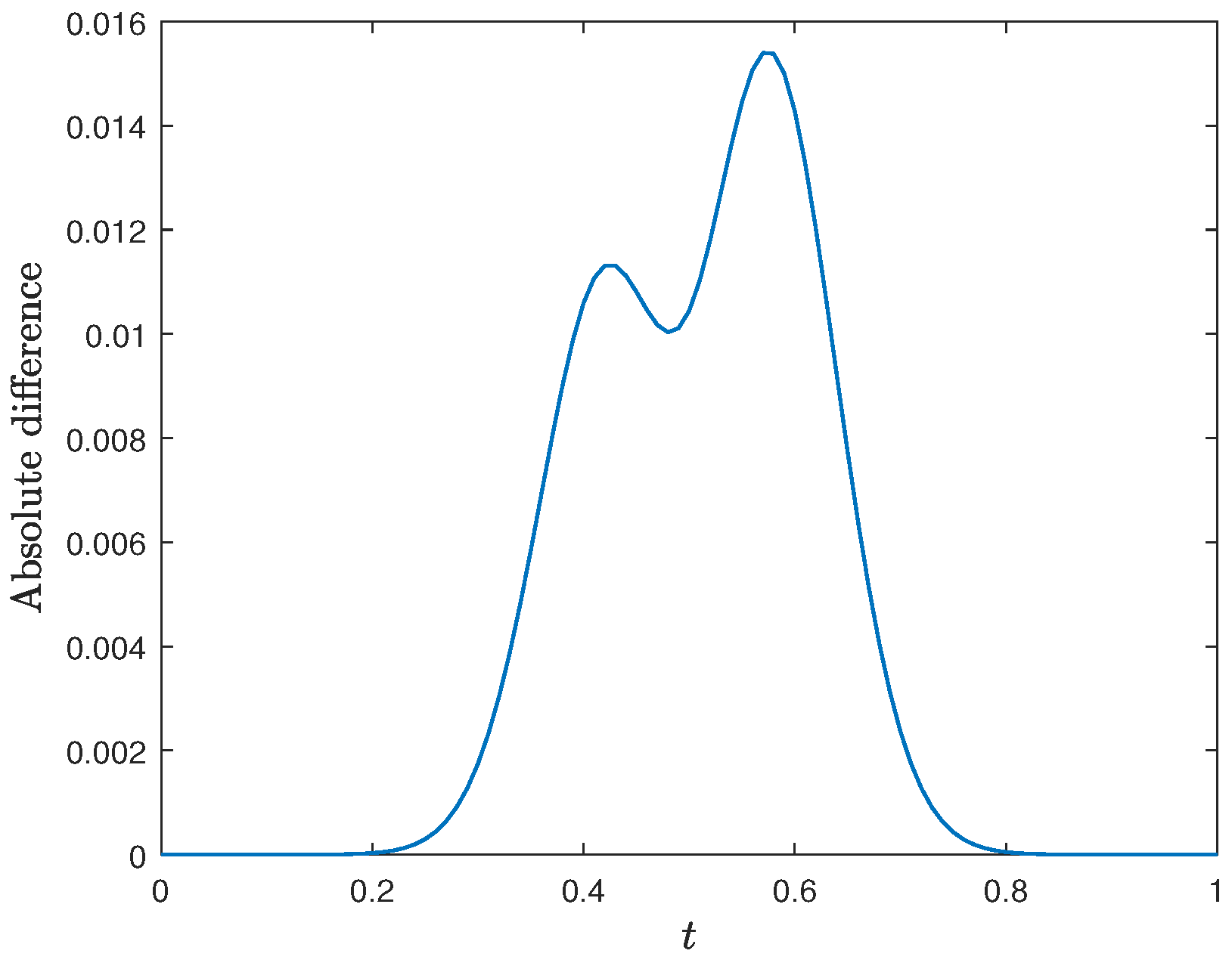
8. Implementation of the UPFD and the HUPFD Schemes on the Linear Schnakenberg Model

The linear Schnakenberg model is given by the equations below:

$$\begin{array}{cc}\hfill {\displaystyle \frac{\partial u}{\partial t}}+c{\displaystyle \frac{\partial u}{\partial x}}& =(q_1-1)u+q_{2}v+{\mu }_1{\displaystyle \frac{{\partial }^{2}u}{\partial x^2}},\hfill \end{array}$$

(118)

$$\begin{array}{cc}\hfill {\displaystyle \frac{\partial v}{\partial t}}+c{\displaystyle \frac{\partial v}{\partial x}}& =-q_{1}u-q_{2}v+{\mu }_1{\displaystyle \frac{{\partial }^{2}v}{\partial x^2}}.\hfill \end{array}$$

(119)

Subject to the following initial and boundary conditions:

$$\begin{array}{c}\hfill \left\{\begin{array}{c}u(x,0)=e^{-x},0\le x\le 10\hfill \\ u(0,t)=e^t,0\le t\le 0.85\hfill \\ u_x(10,t)=-u(10,t),0\le t\le 0.85\hfill \end{array}\right.\end{array}$$

(120)

and:

$$\begin{array}{c}\hfill \left\{\begin{array}{c}v(x,0)=e^{-x},0\le x\le 10\hfill \\ v(0,t)=e^t,0\le t\le 0.85\hfill \\ v_x(10,t)=-v(10,t),0\le t\le 0.85\hfill \end{array}\right.\end{array}$$

(121)

with constants $s=5,c=0,q_1=q_2=0,{\mu }_1=1,{\mu }_2=5$.

8.1. Solving the Linear Schnakenberg Model Using the UPFD Scheme

The linear Schnakenberg model is solved by using the UPFD. Since the coefficient of ${\displaystyle \frac{\partial u}{\partial x}}$ in Equation (14) is positive, we use Equations (5b)–(7) to find the UPFD scheme. Therefore, the UPFD discretization of Equation (14) is given by the equation below:

$$\begin{array}{cc}\hfill {\displaystyle \frac{u_i^{n+1}-u_i^n}{\Delta t}}+c{\displaystyle \frac{u_i^{n+1}-u_i^n}{\Delta x}}& =(q_1-1)u_i^{n+1}+(q_2+s)v_i^n+{\mu }_1\left({\displaystyle \frac{u_{i+1}^n-2u_i^{n+1}+u_{i-1}^n}{{(\Delta x)}^2}}\right),\hfill \end{array}$$

(122)

$$\begin{array}{cc}\hfill {\displaystyle \frac{v_i^{n+1}-v_i^n}{\Delta t}}+c{\displaystyle \frac{v_i^{n+1}-v_i^n}{\Delta x}}& =-q_1{u}_i^{n+1}-q_2{v}_i^{n+1}+{\mu }_2\left({\displaystyle \frac{v_{i+1}^n-2v_i^{n+1}+v_{i-1}^n}{{(\Delta x)}^2}}\right).\hfill \end{array}$$

(123)

which simplifies to the following:

$$\begin{array}{cc}\hfill \left({\displaystyle \frac{1}{\Delta t}}+{\displaystyle \frac{c}{\Delta x}}+(q_1-1)+{\displaystyle \frac{2{\mu }_1}{{(\Delta x)}^2}}\right)u_i^{n+1}& =(q_2+s)v_i^n+{\displaystyle \frac{{\mu }_1}{\Delta x}}(u_{i+1}^n+u_{i-1}^n)+{\displaystyle \frac{c}{\Delta x}}{u}_i^n+{\displaystyle \frac{1}{\Delta t}}{u}_i^n,\hfill \\ \hfill \left({\displaystyle \frac{1}{\Delta t}}+{\displaystyle \frac{c}{\Delta x}}+q_2+{\displaystyle \frac{2{\mu }_2}{{(\Delta x)}^2}}\right)u_i^{n+1}& =-q_1{u}_i^{n+1}+{\displaystyle \frac{1}{\Delta t}}{v}_i^n+{\displaystyle \frac{c}{\Delta x}}{v}_i^n+{\displaystyle \frac{{\mu }_2}{{(\Delta x)}^2}}(v_{i+1}^n+v_{i-1}^n).\hfill \end{array}$$

Let $s_1=\left({\displaystyle \frac{1}{\Delta t}}+{\displaystyle \frac{c}{\Delta x}}+(q_1-1)+{\displaystyle \frac{2{\mu }_1}{{(\Delta x)}^2}}\right)$, $s_2=\left({\displaystyle \frac{1}{\Delta t}}+{\displaystyle \frac{c}{\Delta x}}+q_2+{\displaystyle \frac{2{\mu }_2}{{(\Delta x)}^2}}\right)$, and thus:

$$\begin{array}{cc}\hfill u_i^{n+1}& ={\displaystyle \frac{(q_2+s)}{s_1}}{v}_i^n+{\displaystyle \frac{{\mu }_1}{\Delta x{s}_1}}(u_{i+1}^n+u_{i-1}^n)+{\displaystyle \frac{c}{\Delta x{s}_1}}{u}_i^n+{\displaystyle \frac{1}{\Delta t{s}_1}}{u}_i^n,\hfill \end{array}$$

(124)

$$\begin{array}{cc}\hfill v_i^{n+1}& =-{\displaystyle \frac{q_1}{s_2}}{u}_i^{n+1}+{\displaystyle \frac{1}{\Delta t{s}_2}}{v}_i^n+{\displaystyle \frac{c}{\Delta x{s}_2}}{v}_i^n+{\displaystyle \frac{{\mu }_2}{{(\Delta x)}^2{s}_2}}(v_{i+1}^n+v_{i-1}^n).\hfill \end{array}$$

(125)

8.2. Solving the Schnakenberg Model Using the HUPFD1 Scheme

The Schnakenberg model is solved by using the HUPFD1. Since the coefficient of ${\displaystyle \frac{\partial u}{\partial x}}$ in Equation (14) is positive, we use Equations (5b)–(7) to find the HUPFD1 scheme. Therefore, the HUPFD1 discretization of Equation (14) is given by the equations below:

$$\begin{array}{cc}\hfill {\displaystyle \frac{u_i^{n+1}-u_i^n}{\Delta t}}& +c{\displaystyle \frac{u_i^{n+1}-u_{i-1}^n}{\Delta x}}=(q_1-1)u_i^{n+1}+(q_2+s)v_i^n,\hfill \end{array}$$

$$\begin{array}{cc}\hfill & +{\mu }_1\left({\displaystyle \frac{-u_{i+2}^{n+1}+16u_{i+1}^n-30u_i^{n+1}+16u_{i-1}^n-u_{i-2}^{n+1}}{12{(\Delta x)}^2}}\right),\hfill \\ \hfill {\displaystyle \frac{v_i^{n+1}-v_i^n}{\Delta t}}& +c{\displaystyle \frac{v_i^{n+1}-v_{i-1}^n}{\Delta x}}=-q_1{u}_i^{n+1}-q_2{v}_i^{n+1},\hfill \end{array}$$

(126)

$$\begin{array}{cc}\hfill & +{\mu }_2\left({\displaystyle \frac{-v_{i+2}^{n+1}+16v_{i+1}^n-30v_i^{n+1}+16v_{i-1}^n-v_{i-2}^{n+1}}{12{(\Delta x)}^2}}\right).\hfill \end{array}$$

(127)

which are simplified to the following:

$$\begin{array}{c}\hfill d_1{u}_i^{n+1}+d_2{u}_{i+2}^{n+1}+d_2{u}_{i-2}^{n+1}=d_4{u}_i^n+(q_2+s)v_i^n+16d_2{u}_{i+1}^n+d_3{u}_{i-1}^n,\end{array}$$

(128)

$$\begin{array}{c}\hfill p_1{v}_i^{n+1}+p_2{v}_{i+2}^{n+1}+p_2{v}_{i-2}^{n+1}+q_1{u}_i^{n+1}=d_4{v}_i^{n+1}+p_3{v}_{i-1}^n+16p_2{v}_{i+1}^n.\end{array}$$

(129)

where $a_1={\displaystyle \frac{1}{\Delta t}}+{\displaystyle \frac{c}{\Delta x}}+{\displaystyle \frac{30{\mu }_1}{12{(\Delta )}^2}}$, $a_2={\displaystyle \frac{{\mu }_1}{12{(\Delta x)}^2}}$, $a_3={\displaystyle \frac{c}{\Delta x}}+{\displaystyle \frac{16{\mu }_1}{12{(\Delta x)}^2}}$, $a_4={\displaystyle \frac{1}{\Delta t}}$, $p_1={\displaystyle \frac{1}{\Delta t}}+{\displaystyle \frac{c}{\Delta x}}+q_2+{\displaystyle \frac{30{\mu }_2}{12{(\Delta x)}^2}}$, $p_2={\displaystyle \frac{{\mu }_2}{12{(\Delta x)}^2}}$, $p_3={\displaystyle \frac{c}{\Delta x}}+{\displaystyle \frac{16{\mu }_2}{12{(\Delta x)}^2}}$.

Equations (128) and (129), respectively, are simplified to the following:

$$\begin{array}{c}\hfill A_1{u}^{n+1}=B_1{u}^n+d_1^n\mathrm{and}{A}_2{u}^{n+1}=B_2{u}^n+d_2^n,\end{array}$$

(130)

where:

$$\begin{array}{c}\hfill A_1{u}^{n+1}=\left[\begin{array}{ccccccc}{a}_1& 0& a_2& 0& 0& \cdots & 0\\ 0& a_1& 0& a_2& 0& \cdots & ⋮\\ a_2& 0& a_1& 0& a_2& \ddots & ⋮\\ 0& a_2& 0& a_1& 0& \ddots & 0\\ 0& 0& a_2& 0& a_1& \ddots & a_2\\ ⋮& \ddots & \ddots & \ddots & \ddots & \ddots & 0\\ 0& \cdots & \cdots & \cdots & a_2& 0& a_1\end{array}\right]\left[\begin{array}{c}{u}_1^{n+1}\\ u_2^{n+1}\\ u_3^{n+1}\\ ⋮\\ ⋮\\ ⋮\\ u_{m-1}^{n+1}\\ u_m^{n+1}\end{array}\right]\end{array}$$

(131)

$$\begin{array}{c}\hfill B_1{u}^n=\left[\begin{array}{ccccccc}{a}_4& 16a_2& 0& 0& 0& \cdots & 0\\ a_3& a_4& 16a_2& 0& 0& \cdots & ⋮\\ 0& a_3& a_4& 16a_2& 0& \ddots & ⋮\\ 0& 0& a_3& a_4& 16a_2& \ddots & 0\\ 0& 0& 0& d_3& a_4& \ddots & 0\\ ⋮& \ddots & \ddots & \ddots & \ddots & \ddots & 16a_2\\ 0& \cdots & \cdots & \cdots & 0& a_3& a_4\end{array}\right]\left[\begin{array}{c}{u}_1^n\\ u_2^n\\ u_3^n\\ ⋮\\ ⋮\\ ⋮\\ u_{m-1}^n\\ u_m^n\end{array}\right]\end{array}$$

(132)

and:

$$\begin{array}{c}\hfill d_1^n=a_2\left[\begin{array}{c}{u}_0^n\\ 0\\ 0\\ ·\\ ·\\ ·\\ ·\\ ·\\ ·\\ ·\\ ·\\ u_M^n\end{array}\right]-a_3\left[\begin{array}{c}{u}_0^{n+1}\\ 0\\ 0\\ ·\\ ·\\ ·\\ ·\\ ·\\ ·\\ ·\\ ·\\ u_{m+1}^{n+1}\end{array}\right]\end{array}$$

(133)

and:

$$\begin{array}{c}\hfill A_2{u}^{n+1}=\left[\begin{array}{ccccccc}{p}_1& 0& p_2& 0& 0& \cdots & 0\\ 0& p_1& 0& p_2& 0& \cdots & ⋮\\ p_2& 0& p_1& 0& p_2& \ddots & ⋮\\ 0& p_2& 0& p_1& 0& \ddots & 0\\ 0& 0& p_2& 0& p_1& \ddots & p_2\\ ⋮& \ddots & \ddots & \ddots & \ddots & \ddots & 0\\ 0& \cdots & \cdots & \cdots & p_2& 0& p_1\end{array}\right]\left[\begin{array}{c}{v}_1^{n+1}\\ v_2^{n+1}\\ v_3^{n+1}\\ ⋮\\ ⋮\\ ⋮\\ v_{m-1}^{n+1}\\ v_m^{n+1}\end{array}\right]\end{array}$$

(134)

$$\begin{array}{c}\hfill B_2{u}^n=\left[\begin{array}{ccccccc}{d}_4& 16p_2& 0& 0& 0& \cdots & 0\\ p_3& d_4& 16p_2& 0& 0& \cdots & ⋮\\ 0& p_3& d_4& 16p_2& 0& \ddots & ⋮\\ 0& 0& p_3& d_4& 16p_2& \ddots & 0\\ 0& 0& 0& p_3& d_4& \ddots & 0\\ ⋮& \ddots & \ddots & \ddots & \ddots & \ddots & 16p_2\\ 0& \cdots & \cdots & \cdots & 0& p_3& d_4\end{array}\right]\left[\begin{array}{c}{v}_1^n\\ v_2^n\\ v_3^n\\ ⋮\\ ⋮\\ ⋮\\ v_{m-1}^n\\ v_m^n\end{array}\right]\end{array}$$

(135)

and:

$$\begin{array}{c}\hfill d_2^n=a_2\left[\begin{array}{c}{v}_0^n\\ 0\\ 0\\ ·\\ ·\\ ·\\ ·\\ ·\\ ·\\ ·\\ ·\\ v_m^n\end{array}\right]-a_3\left[\begin{array}{c}{u}_0^{n+1}\\ 0\\ 0\\ ·\\ ·\\ ·\\ ·\\ ·\\ ·\\ ·\\ ·\\ v_{m+1}^{n+1}\end{array}\right]\end{array}$$

(136)

respectively, where u is the unknown vector of the order $m\times 1$ at any time level $t^{n+1}$ and A and B are the coefficient square matrix of order $m\times m$ with a triangular structure.

8.3. Solving the Schnakenberg Model Using the HUPFD2 Scheme

The Schnakenberg model is solved by using the HUPFD2. Since the coefficient of ${\displaystyle \frac{\partial u}{\partial x}}$ in Equation (14) is positive, we use Equations (5b)–(7) to find the HUPFD2 scheme. Therefore, the HUPFD2 discretization of Equation (14) is given by the equation below:

$$\begin{array}{cc}\hfill {\displaystyle \frac{u_i^{n+1}-u_i^n}{\Delta t}}& +c{\displaystyle \frac{u_{i+1}^{n+1}-u_{i-1}^n}{\Delta x}}=(q_1-1)u_i^{n+1}+(q_2+s)v_i^n\hfill \end{array}$$

$$\begin{array}{cc}\hfill & +{\mu }_1\left({\displaystyle \frac{-u_{i+2}^{n+1}+16u_{i+1}^n-30u_i^{n+1}+16u_{i-1}^n-u_{i-2}^{n+1}}{12{(\Delta x)}^2}}\right)\hfill \\ \hfill {\displaystyle \frac{v_i^{n+1}-v_i^n}{\Delta t}}& +c{\displaystyle \frac{v_{i+1}^{n+1}-v_{i-1}^n}{\Delta x}}=-q_1{u}_i^{n+1}-q_2{v}_i^{n+1}\hfill \end{array}$$

(137)

$$\begin{array}{cc}\hfill & +{\mu }_2\left({\displaystyle \frac{-v_{i+2}^{n+1}+16v_{i+1}^n-30v_i^{n+1}+16v_{i-1}^n-v_{i-2}^{n+1}}{12{(\Delta x)}^2}}\right)\hfill \end{array}$$

(138)

which are simplified to the following:

$$\begin{array}{c}\hfill b_1{u}_i^{n+1}+b_2{u}_{i+1}^{n+1}+b_3{u}_{i+2}^{n+1}+b_3{u}_{i-2}^{n+1}=b_4{u}_i^n+b_5{u}_{i-1}^n+16b_3{u}_{i+1}^n,\end{array}$$

(139)

$$\begin{array}{c}\hfill c_1{v}_i^{n+1}+c_2{v}_{i+1}^{n+1}+c_3{v}_{i+2}^{n+1}+c_3{v}_{i-2}^{n+1}=c_4{v}_i^{n+1}+c_4{v}_{i-1}^n+16c_3{v}_{i+1}^n\end{array}$$

(140)

where $b_1={\displaystyle \frac{1}{\Delta t}}-(q_1-1)+{\displaystyle \frac{30{\mu }_1}{12{(\Delta x)}^2}}$, $b_2={\displaystyle \frac{c}{2{(\Delta x)}^2}}$, $b_3={\displaystyle \frac{{\mu }_1}{12{(\Delta x)}^2}}$, $b_4={\displaystyle \frac{1}{\Delta t}}$, $b_5={\displaystyle \frac{c}{2\Delta x}}+{\displaystyle \frac{16{\mu }_1}{12{(\Delta x)}^2}}$, $c_1={\displaystyle \frac{1}{\Delta t}}+q_2+{\displaystyle \frac{30{\mu }_2}{12{(\Delta x)}^2}}$, $c_2={\displaystyle \frac{c}{2\Delta x}}$, $c_3={\displaystyle \frac{{\mu }_2}{12{(\Delta x)}^2}}$, $c_4={\displaystyle \frac{c}{2\Delta x}}+{\displaystyle \frac{16{\mu }_2}{12{(\Delta x)}^2}}$.

Equations (139) and (140) are simplified to the following:

$$\begin{array}{c}\hfill A_1{u}^{n+1}=B_1{u}^n+d_1^n,\end{array}$$

(141)

where:

$$\begin{array}{c}\hfill A_1{u}^{n+1}=\left[\begin{array}{ccccccc}{b}_1& b_2& b_3& 0& 0& \cdots & 0\\ 0& b_1& b_2& b_3& 0& \cdots & ⋮\\ b_3& 0& b_1& b_2& b_3& \ddots & ⋮\\ 0& b_3& 0& b_1& b_2& \ddots & 0\\ 0& 0& b_3& 0& b_1& \ddots & b_3\\ ⋮& \ddots & \ddots & \ddots & \ddots & \ddots & b_2\\ 0& \cdots & \cdots & \cdots & b_3& 0& b_1\end{array}\right]\left[\begin{array}{c}{u}_1^{n+1}\\ u_2^{n+1}\\ u_3^{n+1}\\ ⋮\\ ⋮\\ ⋮\\ u_{m-1}^{n+1}\\ u_m^{n+1}\end{array}\right]\end{array}$$

(142)

$$\begin{array}{c}\hfill B_1{u}^n=\left[\begin{array}{ccccccc}{b}_4& 16b_3& 0& 0& 0& \cdots & 0\\ b_5& b_4& 16b_3& 0& 0& \cdots & ⋮\\ 0& b_5& b_4& 16b_3& 0& \ddots & ⋮\\ 0& 0& b_5& b_4& 16b_3& \ddots & 0\\ 0& 0& 0& b_5& b_4& \ddots & 0\\ ⋮& \ddots & \ddots & \ddots & \ddots & \ddots & 16b_3\\ 0& \cdots & \cdots & \cdots & 0& b_5& b_4\end{array}\right]\left[\begin{array}{c}{u}_1^n\\ u_2^n\\ u_3^n\\ ⋮\\ ⋮\\ ⋮\\ u_{m-1}^n\\ u_m^n\end{array}\right]\end{array}$$

(143)

and:

$$\begin{array}{c}\hfill d_1^n=b_3\left[\begin{array}{c}{u}_0^n\\ 0\\ 0\\ ·\\ ·\\ ·\\ ·\\ ·\\ ·\\ ·\\ ·\\ u_m^n\end{array}\right]-b_3\left[\begin{array}{c}{u}_0^{n+1}\\ 0\\ 0\\ ·\\ ·\\ ·\\ ·\\ ·\\ ·\\ ·\\ ·\\ u_{m+1}^{n+1}\end{array}\right]\end{array}$$

(144)

and:

$$\begin{array}{c}\hfill A_2{u}^{n+1}=\left[\begin{array}{ccccccc}{c}_1& c_2& c_3& 0& 0& \cdots & 0\\ 0& c_1& c_2& c_3& 0& \cdots & ⋮\\ c_3& 0& c_1& c_2& c_3& \ddots & ⋮\\ 0& c_3& 0& c_1& c_2& \ddots & 0\\ 0& 0& c_3& 0& c_1& \ddots & c_3\\ ⋮& \ddots & \ddots & \ddots & \ddots & \ddots & c_2\\ 0& \cdots & \cdots & \cdots & c_3& 0& c_1\end{array}\right]\left[\begin{array}{c}{v}_1^{n+1}\\ v_2^{n+1}\\ v_3^{n+1}\\ ⋮\\ ⋮\\ ⋮\\ v_{m-1}^{n+1}\\ v_m^{n+1}\end{array}\right]\end{array}$$

(145)

$$\begin{array}{c}\hfill B_2{u}^n=\left[\begin{array}{ccccccc}{d}_4& 16c_3& 0& 0& 0& \cdots & 0\\ c_4& d_4& 16c_3& 0& 0& \cdots & ⋮\\ 0& c_4& d_4& 16c_3& 0& \ddots & ⋮\\ 0& 0& c_4& d_4& 16c_3& \ddots & 0\\ 0& 0& 0& c_4& d_4& \ddots & 0\\ ⋮& \ddots & \ddots & \ddots & \ddots & \ddots & 16c_3\\ 0& \cdots & \cdots & \cdots & 0& c_4& d_4\end{array}\right]\left[\begin{array}{c}{v}_1^n\\ v_2^n\\ v_3^n\\ ⋮\\ ⋮\\ ⋮\\ v_{m-1}^n\\ v_m^n\end{array}\right]\end{array}$$

(146)

and:

$$\begin{array}{c}\hfill d_2^n=c_3\left[\begin{array}{c}{v}_0^n\\ 0\\ 0\\ ·\\ ·\\ ·\\ ·\\ ·\\ ·\\ ·\\ ·\\ v_m^n\end{array}\right]-c_3\left[\begin{array}{c}{u}_0^{n+1}\\ 0\\ 0\\ ·\\ ·\\ ·\\ ·\\ ·\\ ·\\ ·\\ ·\\ v_{m+1}^{n+1}\end{array}\right]\end{array}$$

(147)

respectively, where u is the unknown vector of the order $m\times 1$ at any time level $t^{n+1}$ and A and B are the coefficient square matrix of order $m\times m$ with a triangular structure.

8.4. Solving the Schnakenberg Model Using the HUPFD3 Scheme

The Schnakenberg model is solved by using the HUPFD3. Since the coefficient of ${\displaystyle \frac{\partial u}{\partial x}}$ in Equation (14) is positive, we use Equations (5b)–(7) to find the HUPFD3 scheme. Therefore, the HUPFD3 discretization of Equation (14) is given by the equation below:

$$\begin{array}{cc}\hfill {\displaystyle \frac{u_i^{n+1}-u_i^n}{\Delta t}}& +c\left({\displaystyle \frac{-u_{i+1}^n+8u_{i+1}^{n+1}-8u_{i-1}^n+u_{i-2}^{n+1}}{12\Delta x}}\right)=(q_1-1)u_i^{n+1}+(q_2+s)v_i^n\hfill \end{array}$$

$$\begin{array}{cc}\hfill & +{\mu }_1\left({\displaystyle \frac{-u_{i+2}^{n+1}+16u_{i+1}^n-30u_i^{n+1}+16u_{i-1}^n-u_{i-2}^{n+1}}{12{(\Delta x)}^2}}\right),\hfill \end{array}$$

(148)

$$\begin{array}{cc}\hfill {\displaystyle \frac{v_i^{n+1}-v_i^n}{\Delta t}}& +c\left({\displaystyle \frac{-v_{i+1}^n+8v_{i+1}^{n+1}-8v_{i-1}^n+v_{i-2}^{n+1}}{12\Delta x}}\right)=-q_1{u}_i^{n+1}-q_2{v}_i^{n+1}\hfill \end{array}$$

$$\begin{array}{cc}\hfill & +{\mu }_2\left({\displaystyle \frac{-v_{i+2}^{n+1}+16v_{i+1}^n-30v_i^{n+1}+16v_{i-1}^n-v_{i-2}^{n+1}}{12{(\Delta x)}^2}}\right),\hfill \end{array}$$

(149)

which are simplified to the following:

$$\begin{array}{c}\hfill e_1{u}_i^{n+1}+e_2{u}_{i+1}^{n+1}+e_3{u}_{i-2}^{n+1}+e_4{u}_{i+2}^{n+1}=e_5{u}_i^n+q_5{v}_i^n+e_5{u}_{i+2}^n+(8e_3+16e_4)u_{i-1}^n+16e_4{u}_{i+1}^n,\end{array}$$

(150)

$$\begin{array}{c}\hfill f_1{v}_i^{n+1}+q_1{u}_i^{n+1}+8f_2{v}_{i+1}^{n+1}+f_3{v}_{i+2}^{n+1}+f_4{v}_{i-2}^{n+1}=e_5{v}_i^n+16f_3{v}_{i+1}^n+f_2{v}_{i+2}^n+f_5{v}_{i-1}^n,\end{array}$$

(151)

where $e_1={\displaystyle \frac{1}{\Delta t}}-(q_1-1)+{\displaystyle \frac{30{\mu }_1}{12{(\Delta x)}^2}}$, $e_2={\displaystyle \frac{8c}{12\Delta x}}$, $e_3={\displaystyle \frac{c}{12\Delta }}+{\displaystyle \frac{{\mu }_1}{12{(\Delta x)}^2}}$, $e_4={\displaystyle \frac{{\mu }_1}{12{(\Delta x)}^2}}$, $e_5={\displaystyle \frac{1}{\Delta t}}$ $f_1={\displaystyle \frac{1}{\Delta t}}+q_2+{\displaystyle \frac{30{\mu }_2}{12{(\Delta x)}^2}}$, $f_2={\displaystyle \frac{c}{12\Delta x}}$, $f_3={\displaystyle \frac{{\mu }_2}{12{(\Delta x)}^2}}$, $f_4={\displaystyle \frac{c}{12\Delta x}}+{\displaystyle \frac{{\mu }_2}{12{(\Delta x)}^2}}$, $f_5={\displaystyle \frac{8c}{12\Delta x}}+{\displaystyle \frac{16{\mu }_2}{12{(\Delta x)}^2}}$.

Equations (150) and (151) are simplified to the following:

$$\begin{array}{c}\hfill A_1{u}^{n+1}=B_1{u}^n+d_1^n,\end{array}$$

(152)

where:

$$\begin{array}{c}\hfill A_1{u}^{n+1}=\left[\begin{array}{ccccccc}{e}_1& e_2& e_4& 0& 0& \cdots & 0\\ 0& e_1& e_2& e_4& 0& \cdots & ⋮\\ e_3& 0& e_1& e_2& e_4& \ddots & ⋮\\ 0& e_3& 0& e_1& e_4& \ddots & 0\\ 0& 0& e_3& 0& e_1& \ddots & e_4\\ ⋮& \ddots & \ddots & \ddots & \ddots & \ddots & e_2\\ 0& \cdots & \cdots & \cdots & e_3& 0& e_1\end{array}\right]\left[\begin{array}{c}{u}_1^{n+1}\\ u_2^{n+1}\\ u_3^{n+1}\\ ⋮\\ ⋮\\ ⋮\\ u_{m-1}^{n+1}\\ u_m^{n+1}\end{array}\right]\end{array}$$

(153)

$$\begin{array}{c}\hfill B_1{u}^n=\left[\begin{array}{ccccccc}{e}_5& 16e_4& 0& 0& 0& \cdots & 0\\ 8e_3+16e_4& e_5& 16e_4& 0& 0& \cdots & ⋮\\ 0& 8e_3+16e_4& e_5& 16e_4& 0& \ddots & ⋮\\ 0& 0& 8e_3+16e_4& e_5& 16e_4& \ddots & 0\\ 0& 0& 0& 8e_3+16e_4& e_5& \ddots & 0\\ ⋮& \ddots & \ddots & \ddots & \ddots & \ddots & 16e_4\\ 0& \cdots & \cdots & \cdots & 0& 8e_3+16e_4& e_5\end{array}\right]\left[\begin{array}{c}{u}_1^n\\ u_2^n\\ u_3^n\\ ⋮\\ ⋮\\ ⋮\\ u_{m-1}^n\\ u_m^n\end{array}\right]\end{array}$$

and:

$$\begin{array}{c}\hfill d_1^n=e_3\left[\begin{array}{c}{u}_0^n\\ 0\\ 0\\ ·\\ ·\\ ·\\ ·\\ ·\\ ·\\ ·\\ ·\\ u_m^n\end{array}\right]-e_3\left[\begin{array}{c}{u}_0^{n+1}\\ 0\\ 0\\ ·\\ ·\\ ·\\ ·\\ ·\\ ·\\ ·\\ ·\\ u_{m+1}^{n+1}\end{array}\right]\end{array}$$

(154)

and:

$$\begin{array}{c}\hfill A_2{u}^{n+1}=\left[\begin{array}{ccccccc}{f}_1& 8f_2& f_3& 0& 0& \cdots & 0\\ f_4& f_1& 8f_2& f_3& 0& \cdots & ⋮\\ 0& f_4& f_1& 8f_2& f_3& \ddots & ⋮\\ 0& 0& f_4& f_1& 8f_2& \ddots & 0\\ 0& 0& 0& f_4& f_1& \ddots & f_3\\ ⋮& \ddots & \ddots & \ddots & \ddots & \ddots & 8f_2\\ 0& \cdots & \cdots & \cdots & 0& f_4& f_1\end{array}\right]\left[\begin{array}{c}{v}_1^{n+1}\\ v_2^{n+1}\\ v_3^{n+1}\\ ⋮\\ ⋮\\ ⋮\\ v_{m-1}^{n+1}\\ v_m^{n+1}\end{array}\right]\end{array}$$

(155)

$$\begin{array}{c}\hfill B_2{u}^n=\left[\begin{array}{ccccccc}{e}_5& 16f_3& f_2& 0& 0& \cdots & 0\\ f_5& e_5& 16f_3& f_2& 0& \cdots & ⋮\\ 0& f_5& e_5& 16f_3& f_2& \ddots & ⋮\\ 0& 0& f_5& e_5& 16f_3& \ddots & 0\\ 0& 0& 0& f_5& e_5& \ddots & f_2\\ ⋮& \ddots & \ddots & \ddots & \ddots & \ddots & 16f_3\\ 0& \cdots & \cdots & \cdots & 0& f_5& e_5\end{array}\right]\left[\begin{array}{c}{v}_1^n\\ v_2^n\\ v_3^n\\ ⋮\\ ⋮\\ ⋮\\ v_{m-1}^n\\ v_m^n\end{array}\right]\end{array}$$

(156)

and:

$$\begin{array}{c}\hfill d_2^n=f_3\left[\begin{array}{c}{v}_0^n\\ 0\\ 0\\ ·\\ ·\\ ·\\ ·\\ ·\\ ·\\ ·\\ ·\\ v_m^n\end{array}\right]-f_3\left[\begin{array}{c}{u}_0^{n+1}\\ 0\\ 0\\ ·\\ ·\\ ·\\ ·\\ ·\\ ·\\ ·\\ ·\\ v_{m+1}^{n+1}\end{array}\right]\end{array}$$

(157)

respectively, where u is the unknown vector of the order $m\times 1$ at any time level $t^{n+1}$ and A and B are the coefficient square matrix of order $m\times m$ with a triangular structure.

Theorem 1 

(Solution positivity). Let $u^0\left(x\right)\ge 0$, $0\le g^0\left(x\right)\le 1$, $v^0\left(x\right)\ge 0$ for the numerical scheme (18), (37), (124), (125), (128), (129), (139), (140), (150), and (151); we have $u_i^{n+1}\ge 0$, $0\le g_i^{n+1}$, $v_i^{n+1}\ge 0$, independent of the mesh step size [11], where g is the reaction term.

Proof. 

Let us assume that $u_i^{n+1}\ge 0$, $0\le g_i^{n+1}\le 1$, $v_i^n\ge 0$, for $i=0,1,\cdots \cdots ,m$, $n=0,\cdots \cdots m$.

Equations (19), (38), (51), (130), (141), and (152) is composed of a coefficient matrix with strictly diagonally dominant tridiagonal matrix, with positive values on diagonal and subdiagonals, which implies nonnegative inverse. Thus, the solution to the algebraic system is nonnegative $u_i^{n+1}\ge 0$ and $v_i^{n+1}\ge 0$, $i=0,1,\cdots \cdots m$.

Furthermore, it is observed that $g_i^{n+1}\ge 0$ in Equations (19), (38), (51), (130), (141), and (152). By applying the same consideration at each time level, we complete the proof. □

9. Numerical Results

In this section, we present solutions obtained by the positivity-preserving higher-order methods for solving the linear, nonlinear ADR equations and Schnakenberg system of equations. The validity of the method’s outcomes is verified by a comparative analysis with the exact, Crank Nicolson, and NSFD solutions. The performance of the approaches is evaluated by calculating the convergence rates, absolute errors, and computing time. The numerical solution is represented by ${\overline{u}}_{i,j}$, while the analytical solution is denoted by $u_{i,j}$. The error is represented by the symbol $e_{i,j}$, and its magnitude is quantified by the $L_{\infty }$-norm, which is determined by the following formula:

$$\begin{array}{c}\hfill \left|\right|e_{i,n}{\left|\right|}_{\infty }=\left|\right|u_{i,n}-{\overline{u}}_{i,n}{\left|\right|}_{\infty }=Max|u_{i,n}-{\overline{u}}_{i,n}|\end{array}$$

(158)

The convergence rate is calculated by using the formula below:

$$\begin{array}{c}\hfill q={\displaystyle \frac{lo{g}_2\left(\frac{e_k}{e_{k+1}}\right)}{lo{g}_2\left(\frac{\Delta t}{\Delta t_{k+1}}\right)}}\end{array}$$

(159)

9.1. Numerical Results for the Linear Advection–Diffusion–Reaction Equation

Table 1. Convergence rates for the linear ADR equation by the UPFD, NSFD, Crank–Nicolson, and HUPFD with respect to varying $\Delta x$ and $\Delta t$.

		$\mathit{q}\left(\mathit{\Delta }{\mathit{t}}_{\mathit{k}}\right)$
$\Delta {\mathit{t}}_{\mathit{k}}$	$\Delta {\mathit{x}}_{\mathit{k}}$	UPFD	HUPFD 1	HUPFD 2	HUPFD 3	Crank–Nicolson	NSFD
$0.00005$	$0.6667$	$2.1675$	$2.5233$	$1.6978$	$1.0006$	$4.5606$	$2.0579$
$0.0001$	$0.6667$	$0.9973$	$1.0054$	$1.1996$	$1.0212$	$1.0051$	$1.9427$
$0.0002$	$0.6667$	$1.8201$	$1.9990$	$1.5640$	$1.0023$	$2.7372$	$1.8871$
$0.0004$	$0.6667$

presents the convergence rates of the UPFD, Crank–Nicolson, NSFD, and HUPFD solutions with respect to the time and spatial steps. The results show that the HUPFD1 approach shows a faster convergence to the solution compared to the UPFD, HUPFD2, and HUPFD3 approaches. In

Table 2. Numerical results of the linear ADR equation at a fixed $\Delta x=0.6667$ and $\Delta t=0.0001$.

$(\mathit{x},\mathit{t})$	Exact Solution	UPFD Solution	Absolute Error (Exact and UPFD)	HUPFD 1	Absolute Error (Exact and HUPFD 1)	HUPFD 2	Absolute Error (Exact and HUPFD 2)	HUPFD 3	Absolute Error (Exact and HUPFD 3)
$(1.3334,0.0002)$	$0.0048$	$0.0048$	$3.0635\times {10}^{-7}$	$0.0049$	$5.3037\times {10}^{-5}$	$0.0048$	$5.1776\times {10}^{-6}$	$0.0049$	$2.9297\times {10}^{-5}$
$(2.6668,0.0004)$	$0.0185$	$0.0186$	$9.2639\times {10}^{-5}$	$0.0186$	$8.1664\times {10}^{-5}$	$0.0184$	$2.2392\times {10}^{-5}$	$0.0188$	$3.9185\times {10}^{-4}$
$(4.0002,0.0006)$	$0.0709$	$0.0715$	$5.9143\times {10}^{-4}$	$0.0714$	$5.1625\times {10}^{-4}$	$0.0700$	$1.4136\times {10}^{-4}$	$0.0722$	$2.4000\times {10}^{-3}$

, solutions obtained by the exact, UPFD, Crank–Nicolson, NSFD, and HUPFD 1, HUPFD 2, and HUPFD 3 solutions at $(t,x)=\left(1.33334,0.0002\right)$, $\left(2.6668,0.0004\right)$, and $\left(4.0002,0.0006\right)$ are compared.

Table 3. Infinity norm results of the linear ADR equation by using the exact, UPFD, Crank–Nicolson, NSFD, and HUPFD solutions.

$(\mathit{x},\mathit{t})$	Exact	UPFD	Error	HUPFD 1	Error	HUPFD 2	Error	HUPFD 3	Error	Crank Nicolson	Error	NSFD	Error
$u(:,0.0002)$	$1.1654$	$1.1654$	$0.0025$	$1.1654$	$0.0025$	$1.1655$	$0.0025$	$1.1653$	$0.0025$	$1.1654$	$0.0024$	$1.1654$	$0.0025$
$u(:,0.0004)$	$1.1657$	$1.1657$	$0.0026$	$1.1657$	$0.0025$	$1.1657$	$0.0025$	$1.1652$	$0.0027$	$1.1657$	$0.0025$	$1.1657$	$0.0024$
$u(:,0.0006)$	$1.1659$	$1.1660$	$0.0026$	$1.1660$	$0.0026$	$1.1660$	$0.0028$	$1.1652$	$0.0030$	$1.1660$	$0.0025$	$1.1660$	$0.0026$
Time		$0.001230$		$0.002748$		$0.002717$		$0.003089$		$0.002689$		$0.001033$

presents a comparison of the infinite norm results obtained from the HUPDF methods developed in this study, with respect to the Crank Nicolson and NSFD methods, along with their respective computational times. The results show that the UPFD approach exhibits faster convergence to the solution compared to the HUPFD techniques. This is primarily attributed to the fact that the HUPFD methods require an increased number of nodal points for approximating solutions to the problem.

The infinity norms of the proposed HUPFD methods are compared with the UPFD, Crank–Nicolson, and NSFD methods in solving the linear ADR equation, as shown in Table 3. In this example, the results demonstrate that HUPFD approaches preserve the accuracy of the solution. The surface plots of the UPFD, HUPFD1, and exact solutions of linear advection–diffusion–reaction equation are shown in Figure 1a to Figure 2a.

9.2. Numerical Results for the Nonlinear Advection Diffusion Equation

Table 4. Convergence rates for the nonlinear ADR reaction equation by the UPFD and HUPFD with respect to varying $\Delta x$ and $\Delta t$.

		$\mathit{q}\left(\mathit{\Delta }{\mathit{t}}_{\mathit{k}}\right)$
$\Delta {\mathit{t}}_{\mathit{k}}$	$\Delta {\mathit{x}}_{\mathit{k}}$	UPFD	HUPFD	Crank–Nicolson
$0.00005$	$0.6667$	$1.0002$	$1.0029$	$1.9634$
$0.0001$	$0.6667$	$1.0004$	$1.0058$	$1.9055$
$0.0002$	$0.6667$	$1.0007$	$1.0116$	$2.2109$
$0.0004$	$0.6667$

presents the convergence rates of the UPFD and the HUPFD with respect to the time and spatial steps. The convergence rate of HUPFD is slightly higher compared to that of UPFD. The comparison of the exact, UPFD, and HUPFD solutions at $(x,t)=\left(0.3,0.06\right),\left(0.4,0.008\right)$, and $\left(0.5,0.1\right)$ is presented in

Table 5. Numerical results of the nonlinear ADR equation at a fixed $\Delta x=0.01$, $\Delta t=0.05$, $r=0.05$, and $D=0.0002$.

$(\mathit{x},\mathit{t})$	Exact Solution	UPFD Solution	HUPFD Solution	Absolute Error (Exact and UPFD)	Absolute Error (Exact and HUPFD)
$(0.3,0.06)$	$1.327\times {10}^{-7}$	$3.9120\times {10}^{-8}$	$1.314\times {10}^{-7}$	$9.346\times {10}^{-8}$	$1.201\times {10}^{-9}$
$(0.4,0.08)$	$5.27\times {10}^{-7}$	$1.76\times {10}^{-7}$	$5.204\times {10}^{-7}$	$3.509\times {10}^{-7}$	$6.681\times {10}^{-9}$
$(0.5,0.1)$	$1.964\times {10}^{-6}$	$7.322\times {10}^{-7}$	$1.933\times {10}^{-6}$	$1.232\times {10}^{-6}$	$3.195\times {10}^{-8}$
Time		0.006	0.086

. Additionally, the computational time for the UPFD and HUPFD methods are shown. The accuracy of the HUPFD approach is slightly greater in comparison to the UPFD method. However, the UPFD method exhibits low convergence rate as compared to the HUPFD method when solving the linear ADR equation.

The infinity norms of the proposed HUPFD are compared with the UPFD and NSFD methods in solving the linear ADR equation, as shown in

Table 6. Infinity norm results of the nonlinear ADR equation by using the exact, UPFD, NSFD, and HUPFD solutions.

$(\mathit{x},\mathit{t})$	Exact	UPFD	Error	HUPFD	Error	NSFD	Error
$u(:,0.1)$	0.7101	0.6995	0.0106	0.7000	0.0101	0.6994	0.0107
$u(:,0.2)$	0.7101	0.6985	0.0116	0.7000	0.0116	0.6983	0.0118
$u(:,0.4)$	0.7101	0.6979	0.0122	0.7000	0.0122	0.6972	0.0129

. The findings indicate that the HUPFD approach achieved slightly high accuracy (Figure 3 and Figure 4).

Figure 5 show the absolute errors between the exact solution and HUPFD solution for the nonlinear ADR against time.

9.3. Numerical Results for the Schnakenberg Model

Table 7. Convergence rates for the Schnakenberg model by the UPFD, HUPFD 1, HUPFD 2, and HUPFD 3 with respect to varying $\Delta x$ and $\Delta t$.

		$\mathit{q}\left(\mathit{\Delta }{\mathit{t}}_{\mathit{k}}\right)$
$\Delta {\mathit{t}}_{\mathit{k}}$	$\Delta {\mathit{x}}_{\mathit{k}}$	UPFD	HUPFD 1	HUPFD 2	HUPFD 3
$0.00005$	$0.6667$	$1.0002$	$1.0029$	$1.0027$	$1.0027$
$0.0001$	$0.6667$	$1.0004$	$1.0058$	$1.0055$	$1.0055$
$0.0002$	$0.6667$	$1.0007$	$1.0116$	$1.0109$	$1.0109$
$0.0004$	$0.6667$

presents the convergence rates of the UPFD, HUPFD 1, HUPFD 2, and HUPFD 3 in relation to the time and spatial steps. The findings show that the HUPFD methods provide a slightly higher convergence rate compared to the UPFD, HUPFD2, and HUPFD 3 approaches while solving the Schnakenberg model. The solutions of the UPFD, HUPFD 1, HUPFD 2, and HUPFD 3 solutions at $(x,t)=\left(1.33334,0.0002\right),\left(2.6668,0.0004\right)$, and $\left(4.0002,0.0006\right)$ are compared in

Table 8. Comparison of solutions u of the Schnakenberg model by using the UPFD, HUPFD1, HUPFD2, and HUPFD3 solutions.

$(\mathit{x},\mathit{t})$	UPFD	Error	HUPFD 1	Error	HUPFD 2	Error	HUPFD 3	Error
$u(:,0.0002)$	$0.0048$	$0.0013$	$0.0050$	$0.0148$	$0.5254$	$0.0142$	$0.5254$	$0.0142$
$u(:,0.0004)$	$0.0182$	$0.0013$	$0.0198$	$0.0151$	$0.1456$	$0.0146$	$0.1456$	$0.0146$
$u(:,0.0006)$	$0.0690$	$0.0013$	$0.0788$	$0.0154$	$0.0403$	$0.0149$	$0.0403$	$0.0149$
Time	$0.048534$		$0.046653$		$0.057943$		$0.048868$

and

Table 9. Comparison of solutions v of the Schnakenberg model by using the UPFD, HUPFD1, HUPFD2, and HUPFD3 solutions.

$(\mathit{x},\mathit{t})$	UPFD	Error	HUPFD 1	Error	HUPFD 2	Error	HUPFD 3	Error
$u(:,0.0002)$	$0.0048$	$0.0030$	$0.5310$	$0.0186$	$0.5026$	$0.0108$	$0.5271$	$0.0161$
$u(:,0.0004)$	$0.0186$	$0.0029$	$0.1429$	$0.0187$	$0.1350$	$0.0108$	$0.1460$	$0.0163$
$u(:,0.0006)$	$0.0711$	$0.0029$	$0.0390$	$0.0188$	$0.0355$	$0.0108$	$0.0405$	$0.0164$
Time	$0.048534$		$0.046653$		$0.057943$		$0.048868$

. Additionally, the computing times are also provided. The results show that the HUPFD 1 approach has less computational time in comparison to the UPFD, HUPFD 2, and HUPFD 3 solutions when solving the problem. The surface plots of the UPFD, HUPFD1, HUPFD2, and HUPFD3 of the Schnakenberg model are shown in Figure 6a to Figure 7b. The figure demonstrates that the implemented approaches achieve positivity of solution when solving the problem.

10. Conclusions

The HUPFD scheme was developed and used in this study to solve the linear, nonlinear, and system of ADR equations. The goal of this study was to investigate the performance of the HUPFD in various aspects, including stability analysis, consistency, convergence rate, error, computational time, and accuracy. The findings show that the HUPFD performs well as an approximation method to solve the ADR equations, thereby confirming its efficiency and effectiveness. However, it is important to note that the consistency of the HUPFD is conditional. Additionally, we noted that augmenting the order of the UPFD scheme results in an implicit scheme that exhibits conditional stability and enhanced accuracy in terms of time and space. Nevertheless, these schemes also possess certain limitations, including requiring more computational resources than explicit methods. This study has the potential to be extended to a two-dimensional case in order to replicate real-world challenges. It is possible to build higher-order schemes for the time and space fractional advection diffusion equations, which could result in a numerical method that is highly efficient.

References

1. Chen-Charpentier, B.; Kojouharov, H. An unconditionally positivity preserving scheme for advection—Diffusion reaction equations. Math. Comput. Model. 2013, 57, 2177–2185. [Google Scholar] [CrossRef]
2. Bohn, H. Soil absorption of air pollutants. J. Environ. Qual. 1972, 1, 372–377. [Google Scholar] [CrossRef]
3. Guo, Y. Exponential stability analysis of travelling waves solutions for nonlinear delayed cellular neural networks. Dyn. Syst. 2017, 32, 490–503. [Google Scholar] [CrossRef]
4. Britton, N. Others Reaction-Diffusion Equations and Their Applications to Biology; Academic Press: Cambridge, MA, USA, 1986. [Google Scholar]
5. Hao, X.; Liu, L.; Wu, Y. Iterative solution for nonlinear impulsive advection-reaction-diffusion equations. J. Nonlinear Sci. Appl. 2016, 9, 4070–4077. [Google Scholar] [CrossRef]
6. Liu, B.; Allen, M.; Kojouharov, H.; Chen, B. Others Finite-element solution of reaction-diffusion equations with advection. Comput. Methods Water Resour. XI 1996, 1, 3–12. [Google Scholar]
7. Chapwanya, M.; Lubuma, J.; Mickens, R. Nonstandard finite difference schemes for Michaelis-Menten type reaction-diffusion equations. Numer. Methods Partial. Differ. Equ. 2013, 29, 337–360. [Google Scholar] [CrossRef]
8. Khan, H.; Gómez-Aguilar, J.; Khan, A.; Khan, T. Stability analysis for fractional order advection–reaction diffusion system. Phys. A Stat. Mech. Its Appl. 2019, 521, 737–751. [Google Scholar] [CrossRef]
9. Appadu, A. Analysis of the unconditionally positive finite difference scheme for advection-diffusion-reaction equations with different regimes. AIP Conf. Proc. 2016, 1738, 030005. [Google Scholar]
10. Tijani, Y.; Appadu, A. Unconditionally positive NSFD and classical finite difference schemes for biofilm formation on medical implant using Allen-Cahn equation. Demonstr. Math. 2022, 55, 40–60. [Google Scholar] [CrossRef]
11. Ndou, N.; Dlamini, P.; Jacobs, B. Enhanced Unconditionally Positive Finite Difference Method for Advection-Diffusion-Reaction Equations. Mathematics 2022, 10, 2639. [Google Scholar] [CrossRef]
12. Saleh, M.; Kovács, E.; Pszota, G. Testing and improving a non-conventional unconditionally positive finite difference method. Multidiszcip. TudomáNyok Miskolci Egy. KöZleméNye 2020, 10, 206–213. [Google Scholar] [CrossRef]
13. Deville, M.; Fischer, P.; Mund, E. High-Order Methods for Incompressible Fluid Flow; Cambridge University Press: Cambridge, UK, 2002. [Google Scholar]
14. Gassner, G.; Beck, A. On the accuracy of high-order discretizations for underresolved turbulence simulations. Theor. Comput. Fluid Dyn. 2013, 27, 221–237. [Google Scholar] [CrossRef]
15. Bini, D.; Latouche, G.; Meini, B. A family of fast fixed point iterations for M/G/1-type Markov chains. IMA J. Numer. Anal. 2022, 42, 1454–1477. [Google Scholar] [CrossRef]
16. Southworth, B.; Krzysik, O.; Pazner, W.; Sterck, H. Fast Solution of Fully Implicit Runge–Kutta and Discontinuous Galerkin in Time for Numerical PDEs, Part I: The Linear Setting. SIAM J. Sci. Comput. 2022, 44, A416–A443. [Google Scholar] [CrossRef]
17. Chen, J.; Huang, Z. On a fast deterministic block Kaczmarz method for solving large-scale linear systems. Numer. Algorithms 2022, 89, 1007–1029. [Google Scholar] [CrossRef]
18. Gurarslan, G.; Karahan, H.; Alkaya, D.; Sari, M.; Yasar, M. Numerical solution of advection-diffusion equation using a sixth-order compact finite difference method. Math. Probl. Eng. 2013, 2013, 672936. [Google Scholar] [CrossRef]
19. Cui, M. Compact finite difference method for the fractional diffusion equation. J. Comput. Phys. 2009, 228, 7792–7804. [Google Scholar] [CrossRef]
20. Tian, Z.; Ge, Y. A fourth-order compact ADI method for solving two-dimensional unsteady convection—Diffusion problems. J. Comput. Appl. Math. 2007, 198, 268–286. [Google Scholar] [CrossRef]
21. Li, Y.; Kim, J. An efficient and stable compact fourth-order finite difference scheme for the phase field crystal equation. Comput. Methods Appl. Mech. Eng. 2017, 319, 194–216. [Google Scholar] [CrossRef]
22. Li, L.; Jiang, Z.; Yin, Z. Fourth-order compact finite difference method for solving two-dimensional convection—Diffusion equation. Adv. Differ. Equ. 2018, 2018, 234. [Google Scholar] [CrossRef]
23. Visbal, M.; Gaitonde, D. On the use of higher-order finite-difference schemes on curvilinear and deforming meshes. J. Comput. Phys. 2002, 181, 155–185. [Google Scholar] [CrossRef]
24. Carpenter, M.; Gottlieb, D.; Abarbanel, S. The stability of numerical boundary treatments for compact high-order finite-difference schemes. J. Comput. Phys. 1993, 108, 272–295. [Google Scholar] [CrossRef]
25. Vasilyev, O. High order finite difference schemes on non-uniform meshes with good conservation properties. J. Comput. Phys. 2000, 157, 746–761. [Google Scholar] [CrossRef]
26. Chung, Y.; Tucker, P. Accuracy of higher-order finite difference schemes on nonuniform grids. AIAA J. 2003, 41, 1609–1611. [Google Scholar] [CrossRef]
27. Ndou, N.; Dlamini, P.; Jacobs, B. Solving the Advection Diffusion Reaction Equations by Using the Enhanced Higher-Order Unconditionally Positive Finite Difference Method. Mathematics 2024, 12, 1009. [Google Scholar]
28. Calvo, M.; De Frutos, J.; Novo, J. Linearly implicit Runge–Kutta methods for advection–reaction–diffusion equations. Appl. Numer. Math. 2001, 37, 535–549. [Google Scholar] [CrossRef]
29. Zhao, G.; Ruan, S. Time periodic traveling wave solutions for periodic advection–reaction–diffusion systems. J. Differ. Equations 2014, 257, 1078–1147. [Google Scholar] [CrossRef]
30. Dwivedi, K.; Das, S.; Baleanu, D. Numerical solution of nonlinear space–time fractional-order advection–reaction–diffusion equation. J. Comput. Nonlinear Dyn. 2020, 15, 061005. [Google Scholar] [CrossRef]
31. Bennequin, D.; Gander, M.; Gouarin, L.; Halpern, L. Optimized Schwarz waveform relaxation for advection reaction diffusion equations in two dimensions. Numer. Math. 2016, 134, 513–567. [Google Scholar] [CrossRef]
32. Sari, M.; Gürarslan, G.; Zeytinoğlu, A. High-order finite difference schemes for solving the advection-diffusion equation. Math. Comput. Appl. 2010, 15, 449–460. [Google Scholar] [CrossRef]
33. Kovács, E.; Majár, J.; Saleh, M. Unconditionally Positive, Explicit, Fourth Order Method for the Diffusion-and Nagumo-Type Diffusion–Reaction Equations. J. Sci. Comput. 2024, 98, 39. [Google Scholar] [CrossRef]
Figure 1. (a) UPFD solution of the nonlinear ADR equation. (b) HUPFD solution of the linear ADR equation.
Axioms 13 00247 g001
Figure 2. (a) Exact solution of the linear ADR equation. (b) Absolute error obtained by the HUPFD method.
Axioms 13 00247 g002
Figure 3. (a) Analytical solution of the nonlinear ADR equation. (b) HUPFD solution of the nonlinear ADR equation.
Axioms 13 00247 g003
Figure 4. (a) UPFD solution of the nonlinear ADR equation. (b) Comparison of the analytical and numerical solutions of the nonlinear ADR equation.
Axioms 13 00247 g004
Figure 5. Absolute difference between analytical and HUPFD of the nonlinear ADR equation.
Axioms 13 00247 g005
Figure 6. (a) UPFD solution of the Schnakenberg system equations. (b) HUPFD1 solution of the Schnakenberg system equations.
Axioms 13 00247 g006
Figure 7. (a) HUPFD2 solution of the Schnakenberg system equations. (b) HUPFD3 solution of the Schnakenberg system equations.
Axioms 13 00247 g007