
An Extension of the Fréchet Distribution and Applications

 ,
,  , and
, and 
Abstract
1. Introduction
- (a)
- Let . Then its cumulative distribution function (cdf) is
- (b)
- Let . Then .
- (c)
- If , then the rth-moment of X exists for andwhere denotes the gamma function.
- (d)
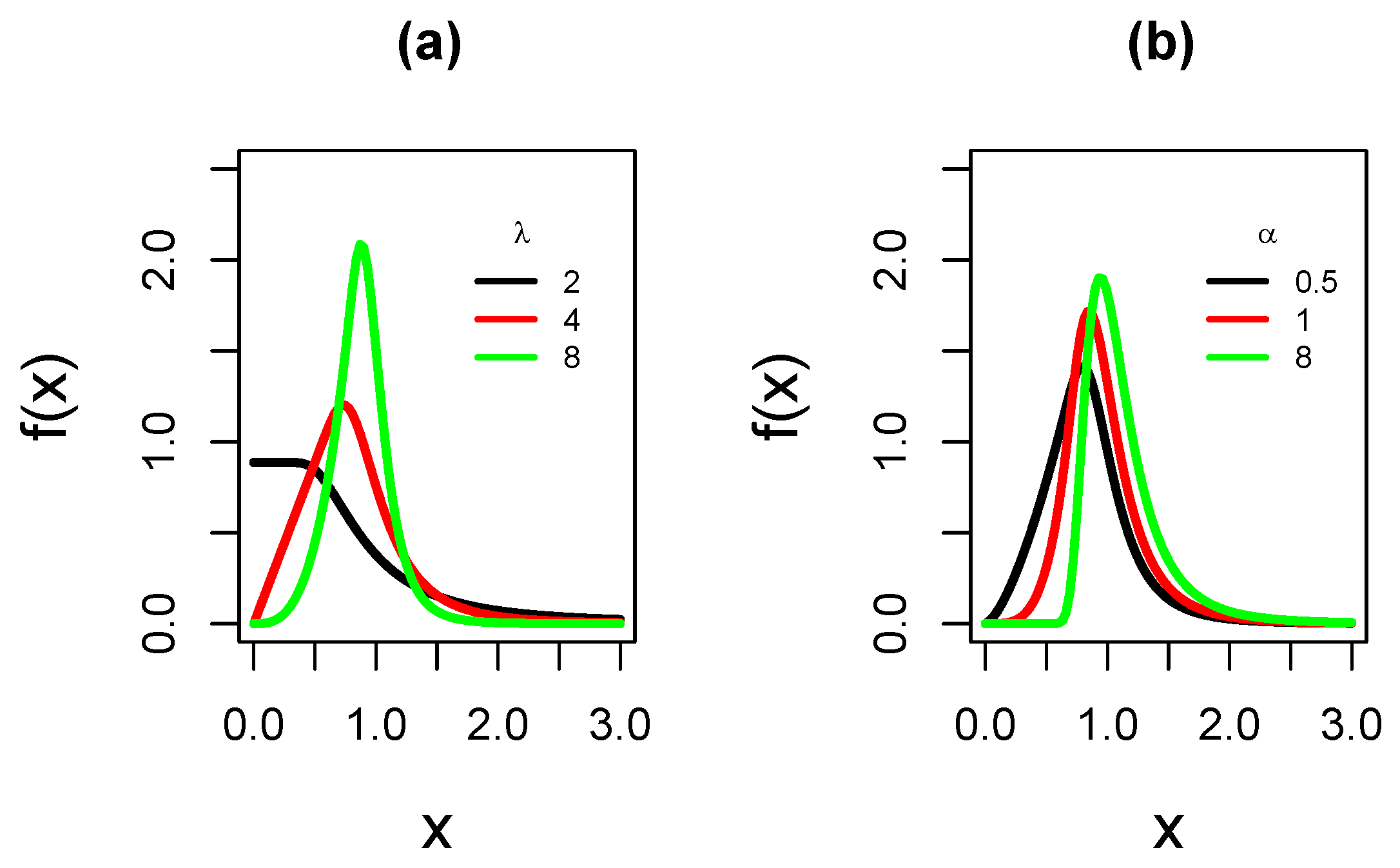
- Let . Then the pdf of X is unimodal with mode or decreasing (for λ close to zero), the hazard function is always unimodal, see [10].
- (a)
- Let . Then the cdf is
- (b)
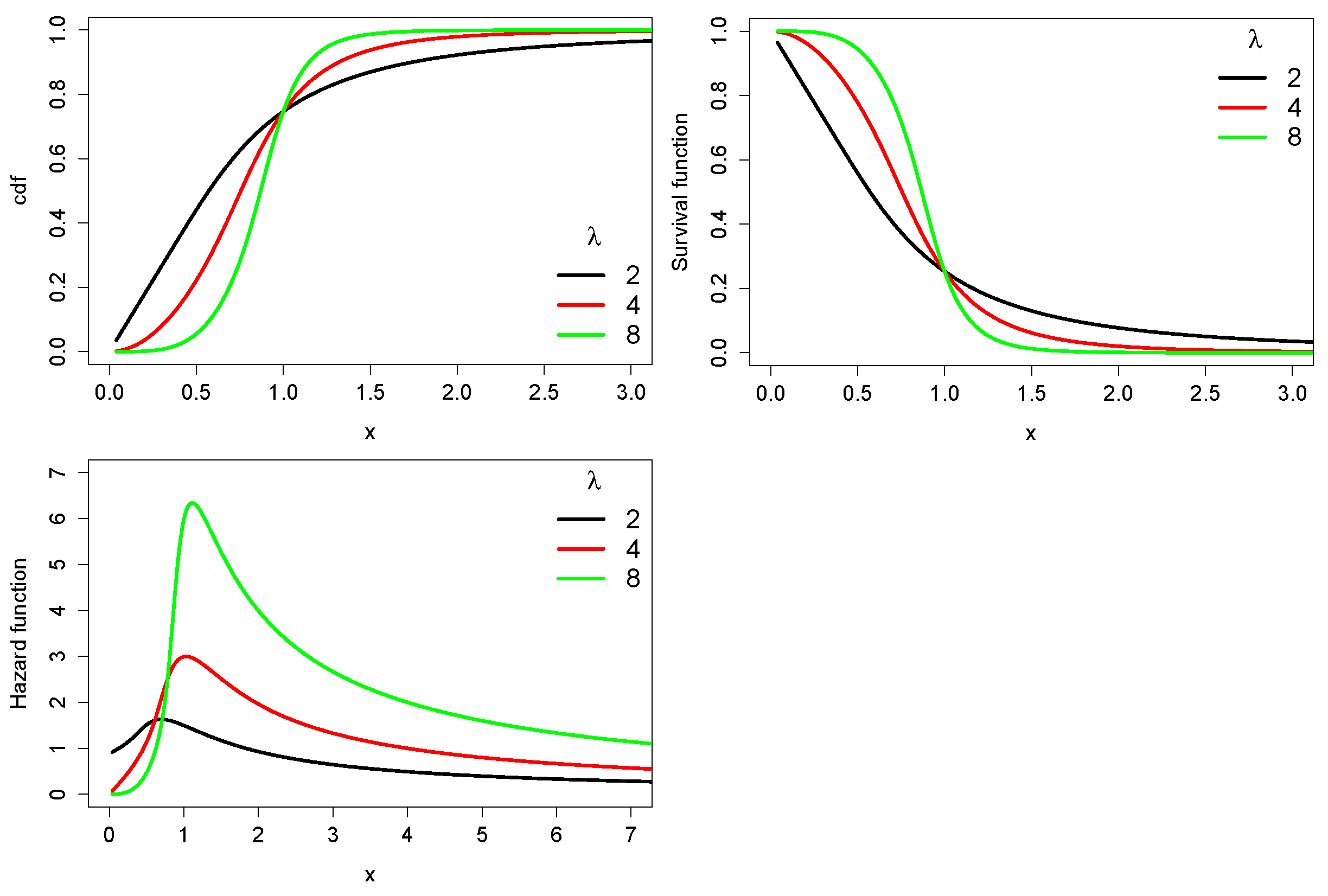
- If then the survival and hazard rate functions are as follows
- (c)
- Let . Then the rth-moment of Y exists for and
2. Results for the SEFr Distribution
2.1. Properties
2.2. Moments
- 1.
- provided that .
- 2.
- provided that .
- 3.
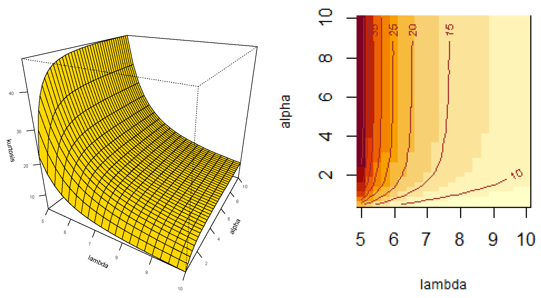
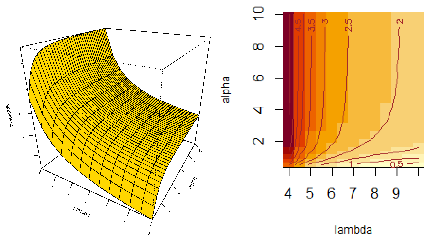
- Let . Then, the skewness, , and kurtosis, , coefficients can be obtained by using
- Shannon Entropy.
2.3. Other Properties of Interest in Reliability
- The reverse hazard rate function.
- The stress-strength parameter.
- Order Statistics.
3. Inference
3.1. ML Estimators
3.2. Observed Fisher Information Matrix
3.3. Simulation Study
| Algorithm 1: To simulate values from the . |
Step 1: Generate and Step 2: Compute Step 3: Compute |
4. Applications
- Slashed Quasi-Gamma, , introduced in [46]. Its pdf is:where , , and .
- Slash Fréchet, , introduced in [20]. Its pdf is:where and is the upper incomplete gamma function.
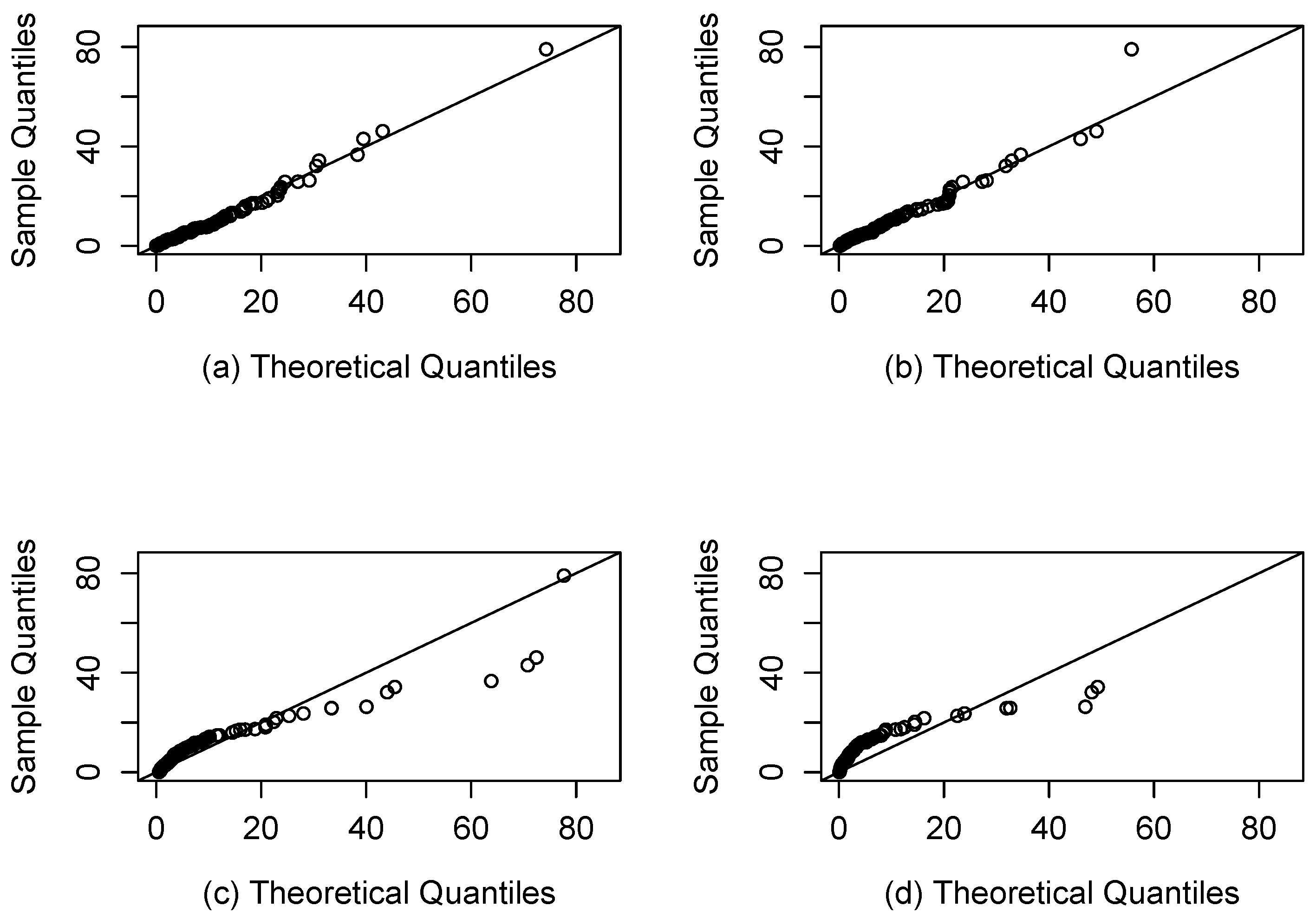
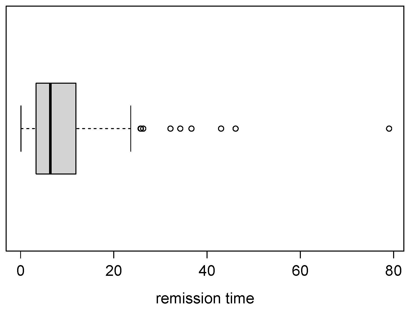
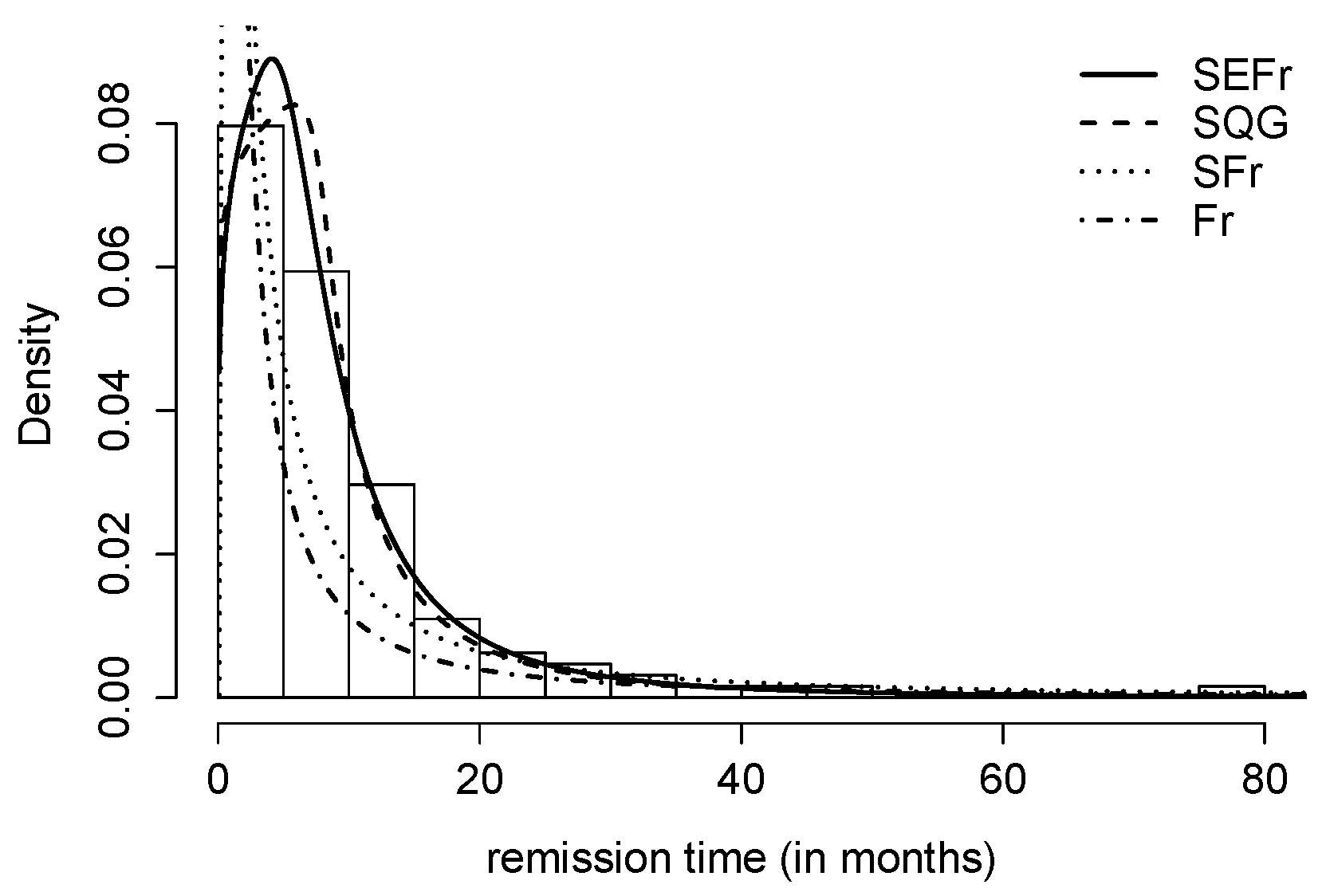
4.1. Application 1 (Patients with Bladder Cancer)
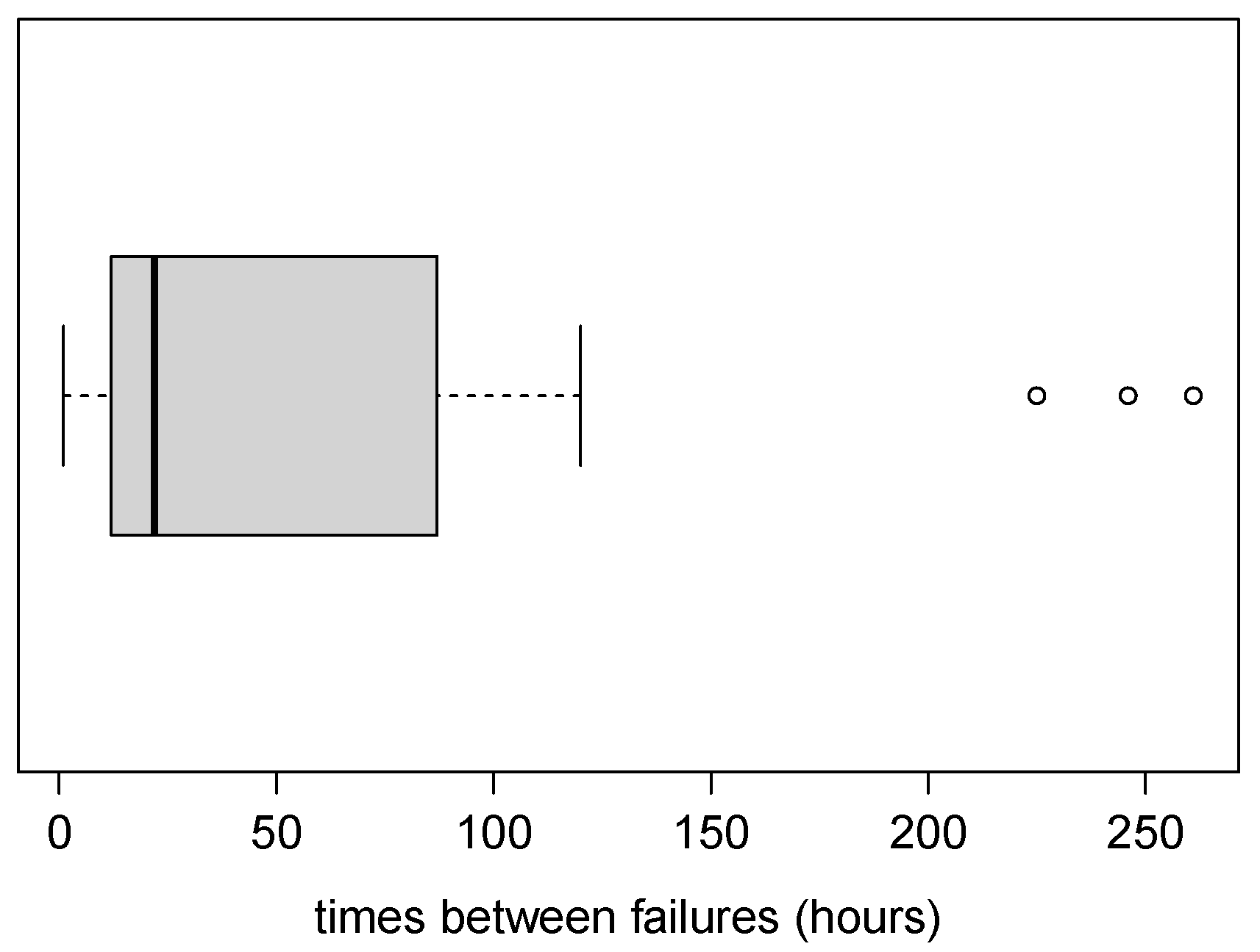
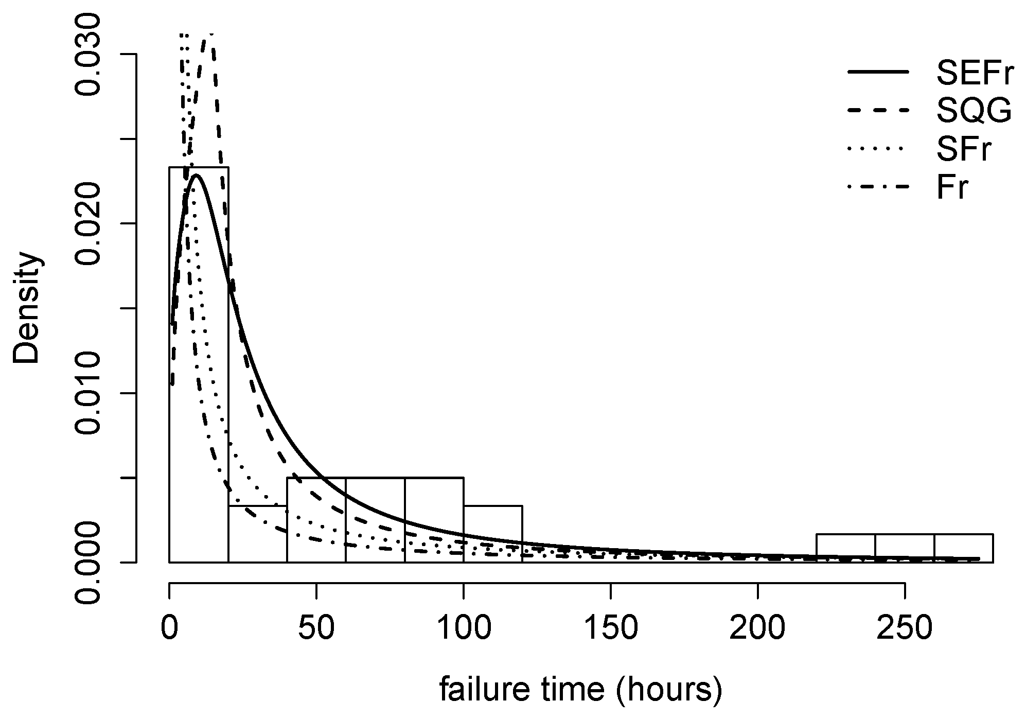
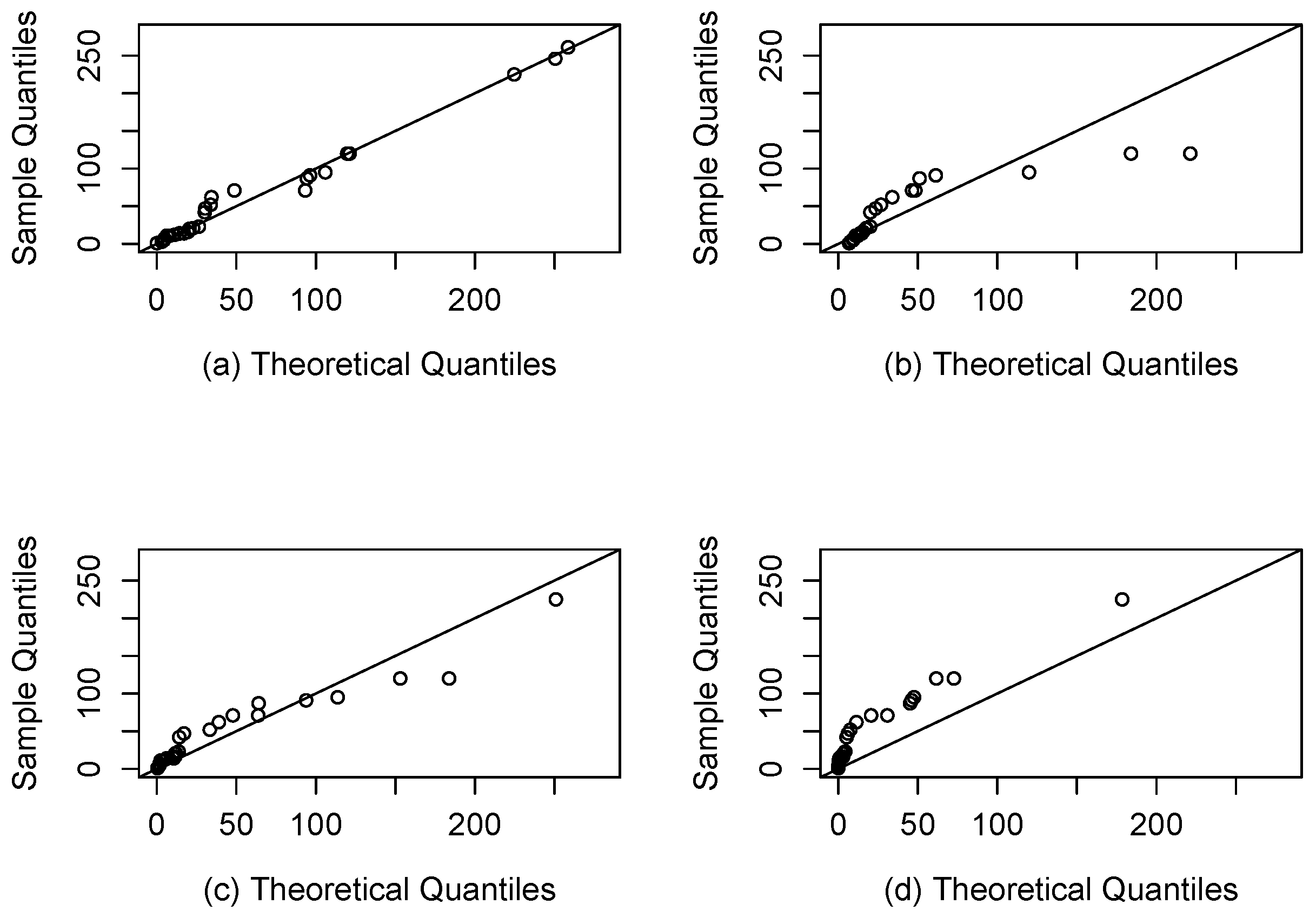
4.2. Application 2 (Air Conditioning System Failures)
5. Conclusions
- The stochastic representation of the new model in terms of the Slash-Exponential is given. In this way, an additional shape parameter is added to Fréchet model.
- Closed expressions for the pdf and cdf are given, therefore also for the survival and hazard rate function.
- It is shown that the new model is unimodal or decreasing. It is proven that if the new shape parameter tends to infinity then the SEFr approaches to Fréchet model.
- Closed expressions are given for the moments, with particular interest on skewness and kurtosis coefficients.
- We highlight that the new model presents less kurtosis than the basal Fréchet distribution. For the best of our understanding, it is the first time in literature that, as result of applying slash methodology, the new model exhibits a lighter right tail and less kurtosis compared to basal model.
- Maximum likelihood method has been proposed to estimate the parameters in the model. Score equations and the observed Fisher information matrix are studied.
- A simulation study has been carried out. There, bias, standard error, RMSE and empirical coverage probability for MLEs have been obtained for increasing sample size. The good asymptotic properties of MLEs can be seen.
- Two real applications are included where the SEFr model is compared to Fr, Slashed Quasi-Gamma and Slash-Fréchet. By using AIC and BIC, it has been seen that the new model provides a better fit compared to others.
Author Contributions
Funding
Data Availability Statement
Conflicts of Interest
References
- Fréchet, M. Sur la loi de probabilité de l’écart maximum. Ann. Soc. Polon. Math. 1927, 6, 93. [Google Scholar]
- Fisher, R.A.; Tippett, L.H.C. Limiting forms of the frequency distribution of the largest and smallest member of a sample. Proc. Camb. Philos. Soc. 1928, 24, 180–190. [Google Scholar] [CrossRef]
- Gumbel, E.J. Statistics of Extremes; Columbia University Press: New York, NY, USA, 1958. [Google Scholar]
- Embrechts, P.; Klüppelberg, C.; Mikosch, T. Modelling Extremal Events for Insurance and Finance; Springer: Berlin, Germany, 1997. [Google Scholar]
- Resnick, S.I. Extreme Values, Regular Variation and Point Processes; Springer: Berlin, Germany, 1987. [Google Scholar]
- Haan, L.; Ferreira, A. Extreme Value Theory: An Introduction; Springer: Berlin/Heidelberg, Germany, 2007. [Google Scholar]
- Kotz, S.; Nadarajah, S. Extreme Value Distributions: Theory and Applications; Imperial College Press: London, UK, 2000. [Google Scholar]
- Gupta, R.C.; Gupta, P.L.; Gupta, R.D. Modeling failure time data by Lehman alternatives. Commun. Stat. Methods 1998, 27, 887–904. [Google Scholar] [CrossRef]
- Coles, S. An Introduction to Statistical Modeling of Extreme Values; Springer: London, UK, 2001. [Google Scholar]
- Ramos, P.L.; Louzada, F.; Ramos, E.; Dey, S. The Fréchet distribution: Estimation and application—An overview. J. Stat. Manag. Syst. 2020, 23, 549–578. [Google Scholar] [CrossRef]
- Calabria, R.; Pulcini, G. Confidence limits for reliability and tolerance limits in the inverse Weibull distribution. Reliab. Eng. Syst. Saf. 1989, 24, 77–85. [Google Scholar] [CrossRef]
- Maswadah, M. Conditional confidence interval estimation for the inverse Weibull distribution based on censored generalized order statistics. J. Stat. Comput. Simul. 2003, 73, 887–898. [Google Scholar] [CrossRef]
- Salman, M.A.W.M.K.; Amer, S.S.M. Order statistics from inverse Weibull distribution and characterizations. Metron 2003, 61, 389–401. [Google Scholar]
- Abbas, K.; Tang, Y. Analysis of Fréchet distribution using reference priors. Commun. Stat. Theory Methods 2015, 44, 2945–2956. [Google Scholar] [CrossRef]
- Punathumparambath, B. Slash Exponential Distribution: Theory and Applications. Bull. Math. Stat. Res. 2020, 8, 38–49. [Google Scholar]
- Abramowitz, M.; Stegun, I.A. Handbook of Mathematical Functions with Formulas, Graphs, and Mathematical Tables. In National Bureau of Standards Applied Mathematics Series 55; United State Department of Commerce: Washington, DC, USA, 1968. [Google Scholar]
- Gupta, R.D.; Kundu, D. Generalized Exponential Distributions. Aust. New Zealand J. Stat. 1999, 41, 173–188. [Google Scholar] [CrossRef]
- Gupta, R.D.; Kundu, D. Generalized Exponential Distribution: Different Methods of Estimations. J. Stat. Comput. Simul. 2001, 69, 315–337. [Google Scholar] [CrossRef]
- Astorga, J.M.; Gómez, H.W.; Bolfarine, H. Slashed generalized exponential distribution. Commun. Stat. Theory Methods 2017, 46, 2091–2102. [Google Scholar] [CrossRef]
- Castillo, J.S.; Rojas, M.A.; Reyes, J. A More Flexible Extension of the Fréchet Distribution Based on the Incomplete Gamma Function and Applications. Symmetry 2023, 15, 1608. [Google Scholar] [CrossRef]
- Rogers, W.H.; Tukey, J.W. Understanding some long-tailed symmetrical distributions. Stat. Neerl. 1972, 26, 211–226. [Google Scholar] [CrossRef]
- Andrews, D.F.; Bickel, P.J.; Hampel, F.R.; Huber, P.J.; Rogers, W.H.; Tukey, J.W. Robust Estimates of Location: Survey and Advances; Princeton University Press: Princeton, NJ, USA, 1972. [Google Scholar]
- Gómez, H.W.; Quintana, F.A.; Torres, F.J. A new Family of Slash-Distributions with Elliptical Contours. Stat. Probab. Lett. 2007, 77, 717–725. [Google Scholar] [CrossRef]
- Arslan, O.; Genc, A. A generalization of the multivariate slash distribution. J. Stat. Plan. Inference 2009, 139, 1164–1170. [Google Scholar] [CrossRef]
- Reyes, J.; Barranco-Chamorro, I.; Gómez, H.W. Generalized modified slash distribution with applications. Commun. Stat. Theory Methods 2020, 49, 2025–2048. [Google Scholar] [CrossRef]
- Del Castillo, J.M. Slash distributions of the sum of independent logistic random variables. Stat. Probab. Lett. 2016, 110, 111–118. [Google Scholar] [CrossRef]
- Zörnig, P. On Generalized Slash Distributions: Representation by Hypergeometric Functions. Stats 2019, 2, 371–387. [Google Scholar] [CrossRef]
- Olmos, N.M.; Varela, H.; Bolfarine, H.; Gómez, H.W. An extension of the generalized half-normal distribution. Stat. Pap. 2014, 55, 967–981. [Google Scholar] [CrossRef]
- Barranco-Chamorro, I.; Iriarte, Y.A.; Gómez, Y.M.; Astorga, J.M.; Gómez, H.W. A generalized Rayleigh family of distributions based on the modified slash model. Symmetry 2021, 13, 1226. [Google Scholar] [CrossRef]
- Barrios, L.; Gómez, Y.M.; Venegas, O.; Barranco-Chamorro, I.; Gómez, H.W. The Slashed Power Half-Normal Distribution with Applications. Mathematics 2022, 10, 1528. [Google Scholar] [CrossRef]
- Gui, W. Statistical properties and applications of the Lindley slash distribution. J. Appl. Stat. Sci. 2012, 20, 283–298. [Google Scholar]
- Castillo, J.S.; Barranco-Chamorro, I.; Venegas, O.; Gómez, H.W. Slash-Weighted Lindley Distribution: Properties, Inference, and Applications. Mathematics 2023, 11, 3980. [Google Scholar] [CrossRef]
- Lehman, L.E. Elements of Large-Sample Theory; Springer: New York, NY, USA, 1999. [Google Scholar]
- Jones, D. Elementary Information Theory; Clarendon Press: Oxford, UK, 1979. [Google Scholar]
- Awad, A.M. The Shannon entropy of generalized gamma and related distributions. In Proceedings of the First Jordamian Mathematics Conference, Amman, Jordan, 2–4 September 1991; pp. 13–27. [Google Scholar]
- Block, H.; Savits, T.; Singh, V. The reversed hazard rate function. Probab. Eng. Inf. Sci. 1998, 12, 69–70. [Google Scholar] [CrossRef]
- Johnson, R.A. Stress-Strength Models for Reliability. In Handbook of Statistics; North-Holland Press: Amsterdam, The Netherlands, 1988; Volume 7. [Google Scholar]
- Milgram, M. The generalized integro-exponential function. Math. Comput. 1985, 44, 443–458. [Google Scholar] [CrossRef]
- R Core Team. R: A Language and Environment for Statistical Computing; R Foundation for Statistical Computing: Vienna, Austria, 2023; Available online: https://www.R-project.org/ (accessed on 25 March 2024).
- Rohatgi, V.K.; Saleh, A.K. An Introduction to Probability and Statistics, 3rd ed.; John Wiley& Sons: New York, NY, USA, 2001. [Google Scholar]
- Lehman, L.E.; Casella, G. Theory of Point Estimation, 2nd ed.; Springer: New York, NY, USA, 1998. [Google Scholar]
- Wang, W.; Cui, Z.; Chen, R.; Wang, Y.; Zhao, X. Regression analysis of clustered panel count data with additive mean models. Stat. Pap. 2023. [Google Scholar] [CrossRef]
- Luo, C.; Shen, L.; Xu, A. Modelling and estimation of system reliability under dynamic operating environments and lifetime ordering constraints. Reliab. Eng. Syst. Saf. 2022, 218 Pt A, 108136. [Google Scholar] [CrossRef]
- Akaike, H. A new look at the statistical model identification. IEEE Trans. Automat. Contr. 1974, 19, 716–723. [Google Scholar] [CrossRef]
- Schwarz, G. Estimating the dimension of a model. Ann. Stat. 1978, 6, 461–464. [Google Scholar] [CrossRef]
- Iriarte, Y.A.; Varela, H.; Gómez, H.J.; Gómez, H.W. A Gamma-Type Distribution with Applications. Symmetry 2020, 12, 870. [Google Scholar] [CrossRef]
- Lee, E.T.; Wang, J. Statistical Methods for Survival Data Analysis; John Wiley & Sons: New York, NY, USA, 2003; Volume 476. [Google Scholar]
- Proschan, F. Theoretical explanation of observed decreasing failure rate. Technometrics 1963, 5, 375–383. [Google Scholar] [CrossRef]


| 0.253 | 0.042 | 0.010 | 0.003 | |
| 0.368 | 0.063 | 0.016 | 0.005 | |
| 0.587 | 0.110 | 0.027 | 0.009 | |
| 0.632 | 0.123 | 0.031 | 0.010 |
| True Value | n = 50 | n = 100 | n = 200 | ||||||||||||
|---|---|---|---|---|---|---|---|---|---|---|---|---|---|---|---|
| Estimator | Bias | SE | RMSE | CP | Bias | SE | RMSE | CP | Bias | SE | RMSE | CP | |||
| 1.5 | 2 | 0.5 | 0.029 | 0.305 | 0.347 | 90.5 | 0.009 | 0.208 | 0.230 | 90.8 | 0.002 | 0.149 | 0.153 | 93.8 | |
| 0.316 | 0.682 | 2.067 | 94.0 | 0.099 | 0.356 | 0.407 | 95.1 | 0.037 | 0.241 | 0.262 | 93.3 | ||||
| 0.073 | 0.374 | 0.726 | 90.5 | 0.015 | 0.133 | 0.144 | 93.7 | 0.007 | 0.091 | 0.096 | 93.5 | ||||
| 1.2 | −0.037 | 0.253 | 0.291 | 90.6 | −0.025 | 0.177 | 0.196 | 93.8 | −0.006 | 0.122 | 0.124 | 94.9 | |||
| 0.124 | 0.404 | 0.598 | 92.8 | 0.027 | 0.259 | 0.278 | 94.1 | 0.024 | 0.181 | 0.185 | 95.1 | ||||
| 1.523 | 7.629 | 4.558 | 91.2 | 0.427 | 1.460 | 1.795 | 94.8 | 0.077 | 0.328 | 0.436 | 93.8 | ||||
| 4 | 0.5 | −0.010 | 0.149 | 0.176 | 89.1 | −0.004 | 0.106 | 0.109 | 93.3 | −0.003 | 0.074 | 0.077 | 93.9 | ||
| 0.512 | 1.222 | 3.100 | 92.9 | 0.187 | 0.722 | 0.854 | 94.8 | 0.084 | 0.483 | 0.521 | 94.7 | ||||
| 0.104 | 0.443 | 0.715 | 89.9 | 0.019 | 0.137 | 0.155 | 93.5 | 0.008 | 0.092 | 0.094 | 94.1 | ||||
| 1.2 | −0.019 | 0.132 | 0.140 | 92.4 | −0.014 | 0.089 | 0.097 | 95.3 | −0.004 | 0.061 | 0.062 | 94.8 | |||
| 0.256 | 0.810 | 1.023 | 93.4 | 0.096 | 0.527 | 0.583 | 93.1 | 0.049 | 0.362 | 0.368 | 95.2 | ||||
| 1.227 | 6.490 | 4.114 | 91.1 | 0.397 | 1.452 | 2.013 | 92.4 | 0.066 | 0.317 | 0.410 | 94.5 | ||||
| 2 | 3 | 0.7 | −0.018 | 0.242 | 0.262 | 90.9 | −0.005 | 0.170 | 0.183 | 92.9 | −0.002 | 0.120 | 0.125 | 94.3 | |
| 0.259 | 0.733 | 0.946 | 94.6 | 0.108 | 0.472 | 0.518 | 95.3 | 0.065 | 0.323 | 0.343 | 95.6 | ||||
| 0.180 | 0.842 | 1.153 | 92.0 | 0.052 | 0.252 | 0.434 | 94.0 | 0.013 | 0.133 | 0.144 | 93.4 | ||||
| 1 | −0.028 | 0.234 | 0.272 | 91.2 | −0.009 | 0.161 | 0.172 | 95.2 | −0.002 | 0.111 | 0.111 | 95.7 | |||
| 0.180 | 0.631 | 0.820 | 92.2 | 0.068 | 0.416 | 0.439 | 95.3 | 0.040 | 0.286 | 0.297 | 94.8 | ||||
| 0.889 | 4.261 | 3.233 | 91.3 | 0.164 | 0.595 | 0.912 | 93.5 | 0.036 | 0.222 | 0.266 | 94.6 | ||||
| 5 | 0.7 | −0.016 | 0.147 | 0.166 | 91.7 | 0.003 | 0.103 | 0.109 | 94.4 | 0.001 | 0.072 | 0.074 | 94.5 | ||
| 0.442 | 1.238 | 1.679 | 93.5 | 0.218 | 0.797 | 0.885 | 95.7 | 0.105 | 0.538 | 0.561 | 96.1 | ||||
| 0.197 | 0.898 | 1.110 | 91.8 | 0.024 | 0.204 | 0.234 | 93.1 | 0.009 | 0.132 | 0.145 | 93.8 | ||||
| 1 | −0.025 | 0.147 | 0.165 | 92.9 | −0.008 | 0.096 | 0.101 | 93.6 | −0.005 | 0.067 | 0.067 | 94.7 | |||
| 0.267 | 1.045 | 1.305 | 91.7 | 0.117 | 0.690 | 0.737 | 94.6 | 0.081 | 0.480 | 0.513 | 94.0 | ||||
| 0.974 | 6.529 | 3.370 | 92.4 | 0.152 | 0.561 | 0.858 | 93.9 | 0.046 | 0.222 | 0.254 | 95.2 | ||||
| 3 | 1.5 | 0.3 | 0.170 | 0.957 | 1.184 | 88.1 | 0.054 | 0.684 | 0.733 | 92.1 | 0.020 | 0.475 | 0.495 | 94.5 | |
| 0.535 | 0.966 | 3.147 | 93.9 | 0.112 | 0.350 | 0.423 | 94.4 | 0.055 | 0.227 | 0.251 | 95.0 | ||||
| 0.013 | 0.123 | 0.152 | 88.9 | 0.005 | 0.083 | 0.098 | 92.1 | 0.002 | 0.057 | 0.059 | 94.6 | ||||
| 0.9 | −0.033 | 0.689 | 0.766 | 90.6 | −0.014 | 0.487 | 0.526 | 92.8 | −0.006 | 0.340 | 0.338 | 95.0 | |||
| 0.104 | 0.327 | 0.390 | 94.4 | 0.039 | 0.215 | 0.249 | 93.9 | 0.023 | 0.148 | 0.155 | 94.7 | ||||
| 0.622 | 2.755 | 2.598 | 91.7 | 0.142 | 0.544 | 0.807 | 93.4 | 0.034 | 0.189 | 0.209 | 95.2 | ||||
| 3.5 | 0.3 | 0.022 | 0.394 | 0.461 | 89.9 | 0.007 | 0.287 | 0.306 | 92.5 | 0.001 | 0.204 | 0.202 | 95.3 | ||
| 0.923 | 1.649 | 4.378 | 93.2 | 0.289 | 0.832 | 1.182 | 95.2 | 0.093 | 0.524 | 0.547 | 95.5 | ||||
| 0.015 | 0.123 | 0.164 | 88.3 | 0.004 | 0.081 | 0.089 | 92.1 | 0.003 | 0.057 | 0.057 | 94.5 | ||||
| 0.9 | −0.021 | 0.301 | 0.352 | 89.7 | −0.005 | 0.209 | 0.232 | 93.2 | −0.003 | 0.145 | 0.150 | 93.3 | |||
| 0.280 | 0.794 | 1.344 | 93.7 | 0.123 | 0.509 | 0.549 | 95.5 | 0.064 | 0.346 | 0.370 | 95.1 | ||||
| 0.681 | 3.211 | 2.885 | 90.6 | 0.100 | 0.438 | 0.728 | 94.9 | 0.022 | 0.184 | 0.202 | 93.8 | ||||
| n | S | |||
|---|---|---|---|---|
| 128 | 9.366 | 10.508 | 3.287 | 18.483 |
| Parameters | Fr (SE) | SFr (SE) | SQG (SE) | SEFr (SE) |
|---|---|---|---|---|
| - | - | - | 9.9436 (1.3592) | |
| 0.6726 (0.0479) | 0.9242 (0.0688) | - | 1.8586 (0.2660) | |
| - | - | - | 0.6329 (0.1558) | |
| - | - | 7.7993 (0.9893) | - | |
| - | - | 10.8627 (1.3211) | - | |
| - | 0.9623 (0.1302) | 1.5211 (0.2282) | - | |
| log-likelihood | −481.0559 | −448.1104 | −411.7342 | −410.0634 |
| AIC | 964.1118 | 900.2208 | 829.4683 | 826.1268 |
| BIC | 966.9638 | 905.9249 | 838.0244 | 834.6829 |
| n | s | |||
|---|---|---|---|---|
| 30 | 59.6333 | 71.8996 | 1.6914 | 4.9595 |
| Parameters | Fr (SE) | SFr (SE) | SQG (SE) | SEFr (SE) |
|---|---|---|---|---|
| - | - | - | 38.5732 (13.9807) | |
| 0.3924 (0.0601) | 0.9508 (0.3089) | - | 1.0968 (0.2273) | |
| - | - | - | 1.1344 (0.5565) | |
| - | - | 14.7397 (3.1532) | - | |
| - | - | 14.3648 (4.2492) | - | |
| - | 0.4067 (0.0960) | 0.7165 (0.1559) | - | |
| log-likelihood | −177.5930 | −163.9272 | −153.0741 | −152.3953 |
| AIC | 357.1859 | 331.8543 | 312.1481 | 310.7905 |
| BIC | 358.5871 | 334.6567 | 316.3517 | 314.9941 |
Disclaimer/Publisher’s Note: The statements, opinions and data contained in all publications are solely those of the individual author(s) and contributor(s) and not of MDPI and/or the editor(s). MDPI and/or the editor(s) disclaim responsibility for any injury to people or property resulting from any ideas, methods, instructions or products referred to in the content. |
© 2024 by the authors. Licensee MDPI, Basel, Switzerland. This article is an open access article distributed under the terms and conditions of the Creative Commons Attribution (CC BY) license (https://creativecommons.org/licenses/by/4.0/).
Share and Cite
Gómez, Y.M.; Barranco-Chamorro, I.; Castillo, J.S.; Gómez, H.W. An Extension of the Fréchet Distribution and Applications. Axioms 2024, 13, 253. https://doi.org/10.3390/axioms13040253
Gómez YM, Barranco-Chamorro I, Castillo JS, Gómez HW. An Extension of the Fréchet Distribution and Applications. Axioms. 2024; 13(4):253. https://doi.org/10.3390/axioms13040253
Chicago/Turabian StyleGómez, Yolanda M., Inmaculada Barranco-Chamorro, Jaime S. Castillo, and Héctor W. Gómez. 2024. "An Extension of the Fréchet Distribution and Applications" Axioms 13, no. 4: 253. https://doi.org/10.3390/axioms13040253
APA StyleGómez, Y. M., Barranco-Chamorro, I., Castillo, J. S., & Gómez, H. W. (2024). An Extension of the Fréchet Distribution and Applications. Axioms, 13(4), 253. https://doi.org/10.3390/axioms13040253