Federated Learning Incentive Mechanism with Supervised Fuzzy Shapley Value

Abstract

The distributed training of federated machine learning, referred to as federated learning (FL), is discussed in models by multiple participants using local data without compromising data privacy and violating laws. In this paper, we consider the training of federated machine models with uncertain participation attitudes and uncertain benefits of each federated participant, and to encourage all participants to train the desired FL models, we design a fuzzy Shapley value incentive mechanism with supervision. In this incentive mechanism, if the supervision of the supervised mechanism detects that the payoffs of a federated participant reach a value that satisfies the Pareto optimality condition, the federated participant receives a distribution of federated payoffs. The results of numerical experiments demonstrate that the mechanism successfully achieves a fair and Pareto optimal distribution of payoffs. The contradiction between fairness and Pareto-efficient optimization is solved by introducing a supervised mechanism.

1. Introduction

The swift progression of Artificial Intelligence (AI) has caused a considerable surge in the generation of large and diverse datasets. These datasets encompass valuable information and sensitive privacy details from various domains. Notably, data islands and privacy concerns pose significant challenges in harnessing the full potential of these datasets. To address the challenges associated with data islands and data privacy, a distributed machine learning technique known as federated learning (FL) [1,2,3] was introduced by Google in 2016.

Cicceri et al. [4] put forth a proposal for the utilization of FL in healthcare, which is called “DILoCC” and built on the concept of FL and adopts the Distributed Incremental Learning (DIL) methodology to leverage the cooperation between sensing devices to build advanced ICT systems with predictive capabilities, which are capable of saving lives and avoiding economic losses. Furthermore, in realistic heterogeneous data distribution scenarios, the performance of FL applied on non-independent identically distributed (Non-IID) data degrades. Therefore, Zhang et al. [5] proposed federated continual learning (FCL) and Bidirectional Compression and Error Compensation (BCEC) algorithms to enhance the performance of non-IID data as well as to reduce communication overheads by introducing knowledge from other local models. FL enables model training to be performed locally at each node, ensuring that sensitive data remains secure and confidential without being transmitted or leaked. This approach not only maximizes the utilization of data for preferring the safeguarding of delicate data privacy, model training is given precedence [6].

Establishing a robust incentive mechanism is crucial in the FL system to encourage data owners to contribute their data and enhance model accuracy. Addressing free-riding behavior among participants, which can significantly impact the accuracy of the federated model, is a key research topic. Therefore, the development of an effective incentive mechanism holds great value in the FL system. Currently, most of the research work [7,8,9,10] assumes the completion of federated model training in the context of determining the attitudes of federated participants’ participation [11,12,13]. However, in actual model training, due to a variety of reasons, such as limited computational resources, weak economic base, limited energy, etc., it can lead to the participants’ participation attitude being uncertain and not being fully committed to the model training, i.e., the participation attitude is ambiguous.

Building upon the aforementioned points, our objective is to devise an incentive structure that guarantees fair allocation of rewards amidst uncertainty regarding the attitudes of federated participants. Consequently, we construct fuzzy Shapley-valued incentives with a supervisory mechanism under fuzzy conditions, which takes into account both fairness and Pareto efficiency considerations. However, this mechanism will increase the complexity, were the mechanism to be applied to a genuine FL situation, how would one acquire and process information about the attitudes of participants towards participation and how to design and implement the supervision mechanism. Summarizing the paper’s main contributions, they can be expressed thus:

(1)

Amidst the ambiguity and doubt of the participants’ involvement outlooks in FL, this paper proposes a fuzzy Shapley value method that can more accurately assess the degree of participants’ contribution and payoff distribution;

(2)

The clash between equity and Pareto effectiveness must be deliberated, as equity necessitates a fair distribution of payoffs among participants, while Pareto efficiency seeks that no participant’s payoff could increase without jeopardizing the payoffs of other participants;

(3)

This paper guarantees fairness and optimization of Pareto efficiency with consistency and introduces a supervisory mechanism that monitors and adjusts the behavior of participants. To guarantee that participants are treated justly, the allotment of advantages is essential in FL and to maximize the overall payoffs.

The paper is organized in the following way: An overview of the related work in the field is presented in Section 2. Preliminaries, providing necessary background information, are presented in Section 3. The FL incentive mechanism and its design are outlined in Section 4.Verification of the incentive mechanism proposal by means of numerical experiments is carried out in Section 5. A comprehensive discussion of the findings are provided in Section 6. The conclusions of this paper are described in Section 7. Proving the Theorem is given in Appendix A.

2. Related Work

The current landscape of FL incentive mechanism research comprises several prominent theoretical approaches. These include the application of the Stackelberg game [14], contract theory’s tenets [15], auctioning techniques [16], and the incorporation of the Shapley value [17]. This paper provides a comprehensive review of the research literature focusing on the design of incentive mechanisms for FL using the Shapley value. In [18], to evaluate the individual contributions of participants who own the data in training the FL model, a novel Shapley value was introduced, which is based on the contribution metric. In [19], a novel formulation for the Shapley value in FL was suggested, which eliminates the need for extra communication costs, incorporates the value of FL data, and offers incentives to the participants. In their work [20], Wang et al. employed the Shapley value to accurately assess the contribution of each participant in FL. To incentivize data owners to actively participate in federated model training and contribute their data, Liu et al. proposed a blockchain-based peer-to-peer payment system for FL in [21]. In this study [21], a blockchain-based peer-to-peer payment system was introduced for FL with the aim of providing incentives to data owners and promoting their active participation in model training. The main objective of this system is to provide a fair and practical mechanism for allocating payoffs, utilizing the principles of the Shapley value. The paper [22] presented an incentive mechanism derived from the Shapley value, aiming to promote greater participation and data sharing among participants by offering them a fair compensation. Liu et al. proposed the bootstrap-truncated gradient Shapley approach in their work [23], which focuses on the fair valuation of participants’ contributions in FL. This strategy entails reconstructing the FL model by utilizing gradient updates for computing the Shapley value. In the work [24], Nagalapattiet et al. presented a collaborative game framework in which participants exchange gradients and calculate Shapley values to identify individuals with pertinent data. The work [24] presented a cooperative game framework that facilitates the sharing of gradients among participants and utilizes Shapley values to identify individuals with relevant data. Acknowledging the disparities in computing the Shapley value for FL, Fan et al. [25] introduced an innovative comprehensive mechanism for calculating the FL Shapley value, aiming to promote fairness. Additionally, in order to mitigate the communication overhead involved in computing the Shapley value in FL, Fan et al. [26] introduced a federated Shapley value mechanism to evaluate participants’ contributions.

In [27], the authors conducted an investigation into different factors that impact FL. Additionally, they proposed an FL incentive mechanism that leverages an improved Shapley value method. In [28], an incentive design called heterogeneous client selection (IHCS) was proposed to enhance performance and mitigate security risks in FL, an approach that involves assigning a recognition value to each client using the Shapley value and is subsequently utilized to aggregate the probability of participation level. In [29], an incentive mechanism is introduced that combines the Shapley value and Pareto efficiency optimization. This approach entails incorporating a third-party entity to oversee the distribution of federated payoffs. If the payoffs can attain Pareto optimality, they are allocated utilizing the Shapley value methodology.

3. Preliminaries

3.1. Federated Learning Framework

FL is a decentralized machine learning framework designed to address data fragmentation and promote cooperation within the field of AI. The primary goal of FL is to facilitate the training of models without the need for participants’ data to leave their local environments. According to adopt this approach, collaborative model development is achieved while also ensuring the preservation of data privacy, security, and legal compliance. By breaking down barriers and allowing for decentralized training, FL promotes the sharing of knowledge and insights while preserving the confidentiality of individual data sources [1,6].

Let $N=\{1,2,\dots ,n\}$ represent a set of n data participants who participate in the FL process denoted as $\{F_1,F_2,F_3,\dots ,F_n\}$. Each participant possesses their local dataset $\{D_1,D_2,\dots ,D_n\}$. The shared model required for FL is denoted as $M_{FED}$, while $M_{SUM}$ represents the traditional machine learning model. The model accuracy of $M_{FED}$ and $M_{SUM}$ is denoted as $V_{FED}$ and $V_{SUM}$, respectively. We can state that there exists a non-negative number $\delta \ge 0$ such that

$$|V_{FED}-V_{SUM}|<\delta ,$$

(1)

which represents the $\delta$-accuracy loss of the FL algorithm [6].

Figure 1 illustrates the FL framework’s schematic diagram, and training is included can be summarized as follows:

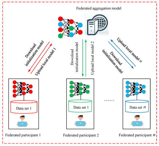
Figure 1. Federated learning framework.

Step 1:

Individual federated participants retrieve the initial global model from the aggregation server.

Step 2:

Each participant trains their local model using the received initial global model.

Step 3:

Upon completing the local model training, participants upload the updated model and associated parameters to the aggregation server.

Step 4:

The aggregation server consolidates the models and parameters uploaded by each participant for the subsequent round of updates.

The widely adopted aggregation approach is the Federated Averaging (FedAvg) algorithm [30], and Steps 2–3 are iteratively performed until the local model reaches convergence.

3.2. Cooperative Games

Consider a cooperative game denoted as $G(N,v)$, which satisfies the following conditions [31]:

$$v(S_1)+v(S_2)\le v(S_1\cup S_2),$$

(2)

$$S_1\cap S_2=⌀,v(⌀)=0.$$

(3)

Here, N denotes a finite group of participants, $S_1,S_2\in 2^N$, and $v:2^N\to \mathbb{R}$ as a game-characteristic function, $2^N$ denotes the set of all subsets of N, $v(S)$ as the payoff function for participants and $v(N)$ as the coalition payoff. Additionally, ${\phi }_i(v)$ represents the payoff of participant i in $v(N)$ and satisfies two specific conditions:

$$v(N)=\sum {\phi }_i(v)\mathrm{and}v(i)\le {\phi }_i(v),\forall i\in N,i=1,2,\dots ,n,$$

(4)

$$v(S)\le \sum _{i\in S}{\phi }_i(v),\forall S\subset N,S\ne ⌀.$$

(5)

Within this context, Equations (4) and (5) are widely recognized as the criteria for individual rationality and coalition rationality, respectively.

3.3. Shapley Value

The Shapley value was the originator of Shapley in cooperative game theory [31], addresses the problem of fair allocation of payoffs in cooperative settings, which defined as follows:

$${\phi }_i(v)=\sum _{i\in S}w(|S|)\left[v(S)-v(S\setminus i)\right],$$

(6)

$$w(|S|)=\frac{(n-|S|)!(|S|-1)!}{n!}.$$

(7)

Let S be a subset of participants, with i being equal to $i=1,2,\dots ,n$, and $S\subset N$, the value $\left|S\right|$ represents the number of subset S. The weight coefficient $w(|S|)$ is associated with the size of $\left|S\right|$. The profit of subset S is denoted as $v(S)$, while $v(S)-v(S\setminus i)$ quantifies the participant $i^{\prime }s$ contribution to coalition S was marginal. Additionally, $v(S\setminus i)$ represents the payoff of participants other than i within subset $\left|S\right|$.

3.4. Fuzzy Coalition of FL

Let $N=\{1,2,\cdots ,n\}$ denote the set consisting of coalition participants in FL, and any subset of the coalition formed by the participants be S, using the fuzzy number $L_{\chi }=\left({\chi }_1,{\chi }_2,\cdots ,{\chi }_n\right)\in {[0,1]}^N$ to denote the degree of participation of a participant i in a subset of the coalition S, i.e., $S(i):L(N)\to {[0,1]}^N$, where $S(i)=0$ denotes that the participant i does not participate in the coalition subset S at all, and $S(i)=1$ denotes that the participant i does participate in the coalition subset S, then $S=\left(S_1,S_2,\cdots ,S_n\right)$ is said to be a fuzzy coalition in FL.

Fuzzy coalitions can help solve the problem of non-cooperativeness in FL, where participants may have selfish motives and tend to keep their data and models. Establishing a fuzzy coalition can lead to the establishment of trust and cooperation among the participants to reach the training goal together. Further, under the fuzzy coalition, the stability and efficiency of the FL system are ensured by designing incentive and punishment mechanisms to motivate the cooperation of the participants.

3.5. Choquet Integral

Let $f:X\to [0,+\infty ),\mu$ is a fuzzy measure defined on X, then the Choquet integral [32,33] of f with respect to $\mu$ is defined as follows:

$${\int }_{X}f(\chi )\circ g(·)={\int }_0^{\infty }g\left(F_{\alpha }\right)d\alpha$$

(8)

When X is a finite set and $f:X\to [0,1]$, the formula for the Choquet integral is redefined as follows:

$$(c)\int fd\mu =\sum _{i=1}^n\left(f\left({\chi }_i\right)-f\left({\chi }_{i-1}\right)\right)\mu \left(A_i\right)$$

(9)

where $F_{\alpha }=\{\chi \mid f(\chi )\ge \alpha ,\chi \in X\}$, $A_i=\left\{{\chi }_i,{\chi }_{i+1},\cdots {\chi }_n\right\}$, $\alpha$ is any number belonging to the group between (0,1], $g(·)$ is the fuzzy density function. In general, assume that $0=f\left({\chi }_0\right)\le f\left({\chi }_1\right)\le f\left({\chi }_2\right)\le \cdots \le f\left({\chi }_n\right)\le 1$. If this relationship is not satisfied, it needs to be readjusted to satisfy the relationship.

In addition, the importance of Choquet integral in FL is reflected in its ability to deal with uncertainty and ambiguity information, integrate and weigh the data, and be able to solve the problem of fair benefit distribution in FL in the case of ambiguity of participants’ attitudes, etc., which can greatly help to improve the accuracy and robustness of federated models.

3.6. Pareto Optimality

Considering $\tilde{\pi }=({\tilde{\pi }}_1,{\tilde{\pi }}_2,\dots ,{\tilde{\pi }}_N):x\to {\mathbb{R}}^N$ as a target vector. For any two solutions $x_i$ and $x_i^{*}$ in x, then Pareto optimality [34] is considered and the following condition holds:

$${\tilde{\pi }}_i(x_1^{*},\cdots ,x_i^{*},\cdots ,x_N^{*})\ge {\tilde{\pi }}_i(x_1,\cdots ,x_i,\cdots ,x_N),\forall i\in N.$$

(10)

This concept aligns with the notion of Pareto optimality, where an allocation is deemed Pareto optimal if there is no alternative allocation that can improve the well-being of one participant without simultaneously worsening the well-being of another participant [35].

3.7. Nash Equilibrium

The participant i’s payoff function is ${\tilde{\pi }}_i(x)$, where $x={\left[x_1,x_2,\cdots ,x_N\right]}^T\in {\mathbb{R}}^N$ represents the vector of actions taken by all participants, and $x_i\in {\mathbb{R}}^n$ represents the action specifically taken by participant i. A Nash equilibrium is a state in which no participant can improve By unilaterally altering their behavior, they increased their income. More specifically, an action profile $x_i^{*}(i=1,\cdots ,n)$ is defined as a Nash equilibrium [36,37], if

$${\tilde{\pi }}_i(x_1^{*},\cdots ,x_i^{*},\cdots ,x_N^{*})\ge {\tilde{\pi }}_i(x_1^{*},\cdots ,x_i,\cdots ,x_N^{*}),\forall i\in N.$$

(11)

4. FL System Incentive Mechanism

4.1. The FL Incentive Model

In establishing the FL incentive model, we base our analysis on the following assumptions:

(1)

Economic Participation: All participants in the FL framework are capable of making financial contributions towards the FL process.

(2)

Participant Satisfaction: The final distribution of payoffs is designed to satisfy all participants.

(3)

Trustworthiness and Integrity: It is assumed that all participants in the FL system are entirely trustworthy and exhibit no instances of cheating or dishonest behavior.

(4)

Multi-Party Agreement: To ensure seamless execution of the FL strategy, it is essential to establish a multi-party agreement.

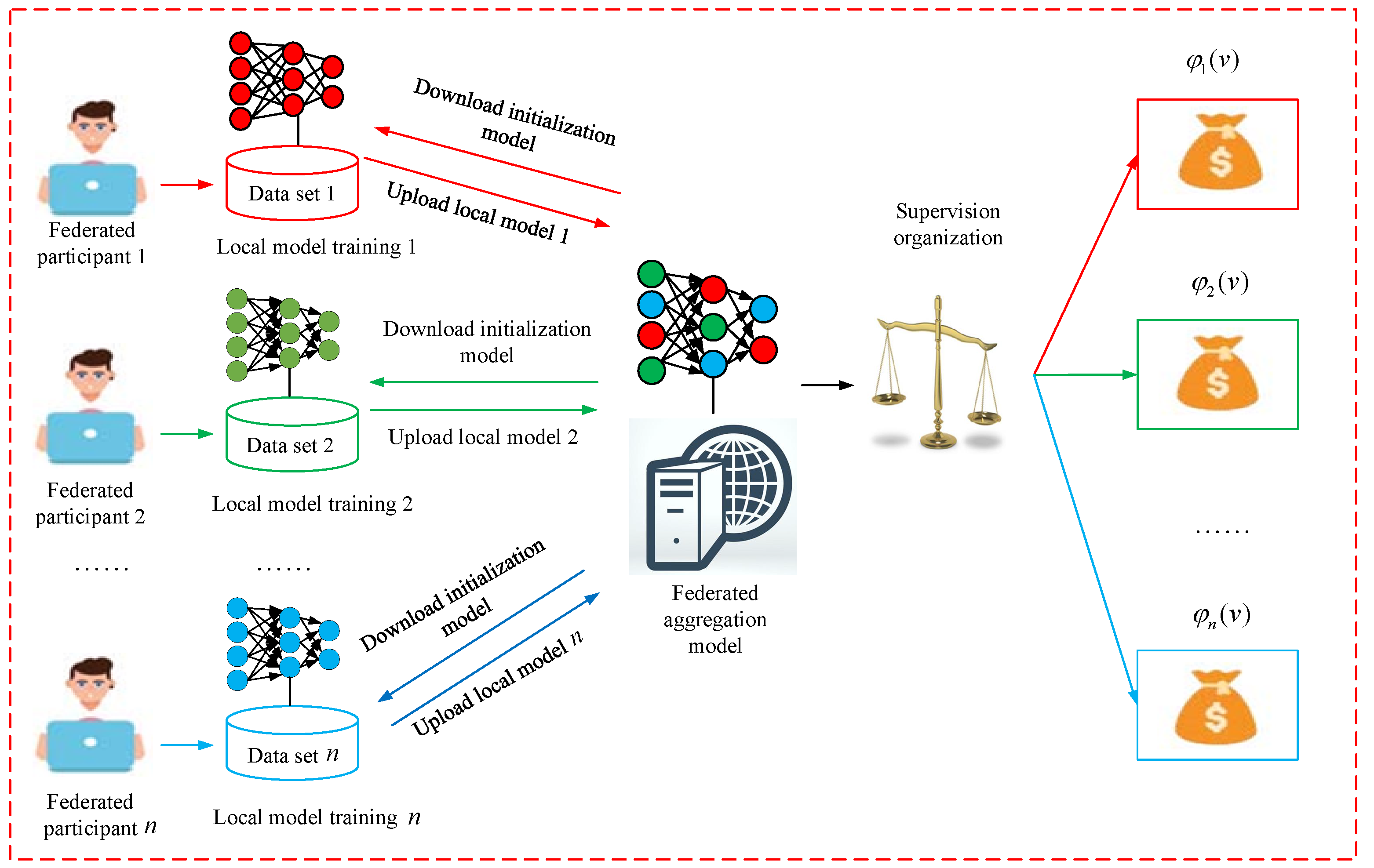
Drawing upon the principles of FL, we put forth a FL incentive model, illustrated in Figure 2. The FL incentive mechanism can be delineated through a sequence of essential steps as follows:

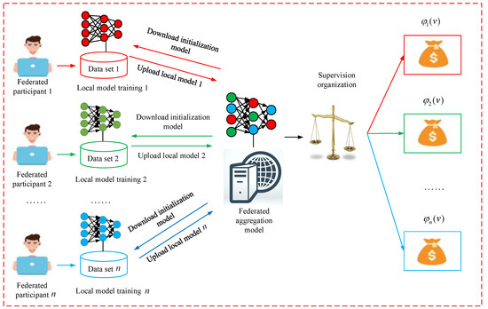
Figure 2. Federated learning incentive model.

Step 1:

Considering n participants in federated model training, each participant possesses its own local dataset, denoted as $D_i$;

Step 2:

Each participant downloads the initialized model from the aggregation server, they independently train the model using their respective local dataset $D_i$, and upload their trained model $m_i$ to the federated aggregation server:

Step 3:

To acquire a fresh global model, the federated aggregation server assumes the responsibility of gathering the model parameters $m_i$, and subsequently employs the federated aggregation algorithm to consolidate these parameters.

Step 4:

The fuzzy Shapley values method is employed to assess the individual contributions of each participant to the global model. This approach allows for the quantification of individual contributions, considering the uncertainty and fuzziness inherent in the participants’ involvement.

Step 5:

The supervising organization assesses the attainment of Pareto optimality for each participant’s payoff. If Pareto optimality is achieved, the fuzzy Shapley value formula is utilized to allocate the payoff. Conversely, the supervising organization imposes penalties on the participant, resulting in the forfeiture of a predetermined fine.

Step 6:

Rewards are allocated to participants who achieve Pareto optimality, as determined by the payoff allocation formula.

4.2. Federated Cost Utility Function

The federated participant $P_i$ needs to take up computational resources such as memory and CPU when performing local model training, and the performance of the participant set P training model $w_G^{*}$ is defined as $F=\{F_1,F_2,F_3,\dots ,F_n\}$, where $F_i$ denotes the participant $P_i$’s local data model training at the CPU clock frequency. In addition, the device of participant $P_i$ has a baseline memory ${\theta }_i$ with an average consumption ratio of ${\beta }_i^t\in [0,1]$, i.e., the actual memory consumption of ${\beta }_i^t{\theta }_i$, in the tth round of local iterations. Assuming the same sample size of input data for each local model iteration and based on the processor quadratic energy model, the computational cost function [13] of the participant $P_i$ in the local model iteration is represented by the following equation:

$$c_{\mathrm{com}}\left(P_i\right)=\alpha \zeta e_i{\gamma }_i{f}_i^2+(1-\alpha ){\beta }_i^t{\theta }_i$$

(12)

Then, define the federated cost utility function of the participant $P_i\in P$ after the rth round of model aggregation as

$$c_i^r(c_{\mathrm{com}}\left(P_i\right))=ln{c}_{\mathrm{com}}\left(P_i\right)$$

(13)

where $\alpha$ denotes the tuning factor used to adjust the computational cost of the participant $P_i$, $\zeta$ denotes the performance of $P_i$’s hardware device used to compute the effective capacitance parameter of the chipset [38], $e_i$ comes to denote the number of CPU cycles required to process a batch of data, and ${\gamma }_i$ denotes the size of data batch samples required for each round of local iteration.

4.3. Model Quality Utility Function

In this paper, the utility assessment of federated participants is defined as two metrics, model quality and freshness [39], and in the classification prediction problem, since the cross-entropy loss function [40,41] outperforms the mean-square error in terms of effectiveness, the cross-entropy loss function $H\left(f\left(y_i\right),z_i\right)=-{\sum }_{i=1}^n{z}_{i}logf\left(y_i\right)$, the labeled data information $\left(y_i,z_i\right)$ can be processed efficiently to improve the accuracy and reliability of the data. To quantify the freshness of the model, the concept of trusted time is introduced, and to ensure the verifiability of the timestamps, the federation participants need to request a timer $T_i^k\left(w_i^k\right)$ from the content container [42] in the Trusted Hardware SGX, after completing the iteration of the local model $w_i^k$. The freshness $F\left(w_i^k\right)$ of the model $w_i^k$ can be defined as $F\left(w_i^k\right)=lg{T}_i^k\left(w_i^k\right)$. Based on this, the quality assessment function $Q\left(w_i^t\right)$ for model $w_i^t$ is defined as

$$Q\left(w_i^t\right)=\frac{{\mu }_{0}F\left(w_i^k\right)}{{\mu }_1+H\left(f\left(x_i\right),z_i\right)},$$

(14)

where the model utility parameters ${\mu }_0,{\mu }_1⩾0$ are set according to the loss function, the neural network structure, and the data distribution [43]. To assess the utility of the participants, adaptive aggregation was used, where the difference between the quality of the model of participant $P_i$ after the rth round of aggregation, $Q\left(w_G^r\left(P_i\right)\right)$, and the quality of the model of those who did not take part in the aggregation, $Q\left(w_G^r\left(P\setminus \left\{P_i\right\}\right)\right)$, was taken as the utility function [44]. Based on the strongly convex function property of the model quality $Q\left(w_i^t\right)$ and the boundary $Q\left(w_i^0\right)$ of the initialized global model, define the utility function of the participant $P_i\in P$ boosted after the rth round of model aggregation as follows:

$$v_i^r(Q\left(P_i\right))={\rho }_i^r\left[Q\left(w_G^r\left(P_i\right)\right)-Q\left(w_G^r\left(P\setminus \left\{P_i\right\}\right)\right)\right],$$

(15)

where ${\rho }_i^r$ then denotes the payoff reward that federated participant $P_i$ receives in the rth round of model aggregation, and if $v_i(r)<0$, it means that $P_i$ needs to pay a price compensation for obtaining a higher-quality model parameter to prevent federated participants from engaging in free-riding behavior.

4.4. Federated Optimization Function

The FL optimization function is known from Formulas (13) and (15):

$$\underset{c_i^r(c_{\mathrm{com}}\left(P_i\right))}{argmax}\sum _{i=1}^n[v_i^r(Q\left(P_i\right))-c_i^r(c_{\mathrm{com}}\left(P_i\right))],c_i^r(c_{\mathrm{com}}\left(P_i\right))\le v_i^r(Q\left(P_i\right)).$$

(16)

4.5. The Fuzzy Shapley Value

According to the fuzzy coalition of FL in Section 3.4, Choquet integral in Section 3.5 and Formulas (8) and (9). Given a fuzzy coalition $S\in R(N)$, let $H(S)=\{S(i)\mid 0<S(i)\le 1,i\in N\},q(S)$ be the number of elements in $H(S)$, and the elements in $H(S)$ be sorted into $f_1\le f_2\le \dots \le f_{q(S)}$ in an ascending sequence. The payoff function $\tilde{v}$ of the fuzzy coalitional cooperation game $(N,\tilde{v},\chi )$ can be expressed as a Choquet integral:

$$\tilde{v}(S)=\int Sd\tilde{v}=\sum _{l=1}^{q(S)}v({\left[S\right]}_{f_l})(f_l-f_{l-1})$$

(17)

Then the fuzzy Shapley value ${\tilde{\phi }}_i(\tilde{v})$ of the fuzzy coalitional cooperation game $(N,\tilde{v})$ can be expressed as follows:

$${\tilde{\phi }}_i(\tilde{v})=\sum _{l=1}^{q(S)}{\phi }_i(v({\left[S\right]}_{f_l}))(f_l-f_{l-1}),i\in {\left[S\right]}_{f_l}\subseteq N$$

(18)

where, $f_0=0,l=1,2,\dots ,q(S)$, ${\left[S\right]}_{f_l}=\{i\in N\mid S(i)\ge f_l\}$ denotes the payoff function for a clear coalition of all participants with participation level $S(i)\ge f_l$, $v({\left[S\right]}_{f_l})$ denotes the payoff function of a clear coalition of all participants with participation level $S(i)\ge f_l$, ${\phi }_i(v({\left[S\right]}_{f_l}))$ denotes the payoff function of a clear coalition of all participants with participation level $S(i)\ge f_l$, and ${\phi }_i(v({\left[S\right]}_{f_l}))$ denotes a clear coalition of all participants with participation level $S(i)\ge f_l$ of the classical Shapley value, $v({\left[S\right]}_{f_l})$ calculated from Formula (15). As with the classical Shapley value, the fuzzy Shapley value satisfies the following theorem:

Theorem 1

(Validity). ${\displaystyle \sum _{i\in N}}{\tilde{\phi }}_i(\tilde{v})=\tilde{v}(N)$.

Theorem 2

(Symmetry). If participants $i,j\in N$ have $\tilde{v}(S\cup \left\{i\right\})=\tilde{v}(S\cup \left\{j\right\})$ for any fuzzy coalition $S\in P(N\setminus \{i,j\})$, then ${\tilde{\phi }}_i(\tilde{v})={\tilde{\phi }}_j(\tilde{v})$.

Theorem 3

(Additivity). For any two fuzzy cooperative games $<N,{\tilde{v}}_1>$ and $<N,{\tilde{v}}_2>$, if there exists a fuzzy cooperative game $<N,{\tilde{v}}_1+{\tilde{v}}_2>$, for any fuzzy coalition $S\in P(N)$, it will always satisfy $({\tilde{v}}_1+{\tilde{v}}_2)(S)={\tilde{v}}_1(S)+{\tilde{v}}_2(S)$, then ${\tilde{\phi }}_i({\tilde{v}}_1+{\tilde{v}}_2)={\tilde{\phi }}_i({\tilde{v}}_1)+{\tilde{\phi }}_i({\tilde{v}}_2)$.

Theorem 4

(Dumbness). If for all fuzzy coalitions S containing participant i, if $\tilde{v}(S)=\tilde{v}(S\setminus \left\{i\right\})$ is satisfied, then ${\tilde{\phi }}_i(\tilde{v})=0$.

Proof. 

The proofs of Theorems 1–4 are given in Appendix A.1, Appendix A.2, Appendix A.3 and Appendix A.4 of the Appendix A. □

4.6. The Conflict of Fairness and Pareto Optimality

Consider a scenario involving n participants, where each participant i has a fuzzy coalition investment denoted as $x_i$. The investment of participant i satisfies $x_i\in (0,\infty )$, $i=1,2,\dots ,n$. The fuzzy coalition investments of all participants can be represented as an n-dimensional vector $x=(x_1,x_2,\dots ,x_n)$. Furthermore, the fuzzy coalition cost investment for participant i is denoted as ${\tilde{c}}_i(x_i)$, which calculated from Formula (13). The function ${\tilde{c}}_i(x_i)$ is assumed to be differentiable, convex, and strictly monotone increasing. It satisfies the following conditions: $\frac{\partial {\tilde{v}}_i(x)}{x_i}>0$, $\frac{{\partial }^2{\tilde{v}}_i(x)}{\partial x_i^2}>0$, ${\tilde{c}}_i(0)=0$. The federated return $\tilde{v}(x_1,x_2,\dots ,x_n)$ calculated from Formulas (8), (9) and (15), which determined by the federated investment decisions made by the n participants. The function is strictly monotonically increasing, differentiable, and concave. It also satisfies the specified conditions: $\frac{\partial {\tilde{v}}_i(x)}{x_i}>0$, $\frac{{\partial }^2{\tilde{v}}_i(x)}{\partial x_i^2}<0$, $\tilde{v}(0,0,\dots ,0)=0$. The allocation of federated payoffs to the n participants follows a specific formula, as described by Equations (17) to (18).

While the fuzzy Shapley value is capable of quantifying the contribution of each participant, it fails to consider the inherent trade-off between fairness and Pareto optimality. Specifically, it overlooks the requirement of achieving Pareto optimization before to the allocation of payoffs. Consequently, it does not effectively address the issue of free-riding behavior among federated participants. Consequently, we put forward the following theorem:

Theorem 5.

While the fuzzy Shapley value method effectively promotes fairness in the distribution of payoffs after FL, it does not sufficiently tackle the problem of optimizing incentives for participants’ investments prior to FL. In other words, it does not achieve Pareto efficiency optimization prior to the commencement of FL.

Proof. 

The proof of this theorem can be found in Appendix A.5 of Appendix A. □

4.7. Introducing Supervisory Organization

The Establishment of Supervised Mechanism

4.7.1. The Implementation of a Supervisory System

The introduction of supervisors to mitigate free riding in the FL process by requiring federated participants to pay a fee to the supervisor proposed in [45]. Holmstrom [46] further emphasized the use of incentive mechanisms to address free riding, with the supervisor playing a crucial role in breaking equilibrium and creating incentives.

Assuming that the supervisor is cognizant of the fact that the federated payoff is such that it exceeds or equals the Pareto optimal payoff, they can distribute this payoff to the participants using the fuzzy Shapley value Formulas (17)–(18). However, if the federated payoffs fall short of the Pareto optimal value, the federated participants will be obligated to pay a specified fee ${\tilde{k}}_i$ in the following manner:

$$\begin{array}{cc}{\tilde{r}}_i(x)=\left\{\begin{array}{c}{\tilde{\phi }}_i(\tilde{v}(x)),\\ {\tilde{\phi }}_i(\tilde{v}(x))-{\tilde{k}}_i,\end{array}\right.\hfill & \begin{array}{c}\mathrm{if}\tilde{v}(x)\ge \tilde{v}(x^{*})\hfill \\ \mathrm{if}\tilde{v}(x)<\tilde{v}(x^{*})\hfill \end{array}\end{array}$$

(19)

where we let $x^{*}=(x_1^{*},x_2^{*},\dots ,x_n^{*})$ be the federated investment vector that satisfies Formula (A4).

4.7.2. Penalty Conditions

Theorem 6.

In the case where the federated investment mechanism $x^{*}=(x_1^{*},x_2^{*},\dots ,x_n^{*})$ meets the criteria of Pareto efficiency and the penalty ${\tilde{k}}_i$ to serve as a Nash equilibrium, it must meet the following conditions:

(1)

If the individual investment $x_i$ of participant i is less than the Pareto optimal federated investment $x_i^{*}$, i.e., e.g., $x_i<x_i^{*}$, and $\tilde{v}(x)$ is a monotonically increasing function (i.e., $\tilde{v}(x_i,x_{n-i}^{*})<\tilde{v}(x_i^{*},x_{n-i}^{*}))$, participant i is fined. The remaining payoff after deducting the fine is denoted as ${\tilde{r}}_i\left[\tilde{v}(x_i,x^{*}n-i)\right]=\tilde{\phi }i(\tilde{v}(x))-{\tilde{k}}_i$, and the profit of participant i can be expressed as follows:

$${\tilde{\pi }}_i\left[\tilde{v}(x_i,x_{n-i}^{*})\right]={\tilde{\phi }}_i(\tilde{v}(x))-{\tilde{k}}_i-{\tilde{c}}_i(x_i),i=1,2,\dots ,n.$$

(20)

(2)

If the individual investment $x_i$ of participant i is equal to the Pareto optimal federated investment $x_i^{*}$, i.e., $x_i=x_i^{*}$, then $\tilde{v}(x)=\tilde{v}(x^{*})$. The remaining payoff after the penalty is ${\tilde{r}}_i\left[\tilde{v}(x_i^{*},x_{n-i}^{*})\right]={\tilde{\phi }}_i(\tilde{v}(x^{*}))$, and the profit of participant i can be expressed as follows:

$${\tilde{\pi }}_i\left[\tilde{v}(x_i^{*},x_{n-i}^{*})\right]={\tilde{\phi }}_i(\tilde{v}(x^{*})-{\tilde{c}}_i(x_i^{*}),i=1,2,\dots ,n.$$

(21)

In this context, $x_{n-i}^{*}=(x_1^{*},\dots x_{i-1}^{*},x_{i+1}^{*},\dots ,x_n^{*})$ denotes the Pareto optimal federated investment vector consisting of $n-i$ participants.

Proof. 

The proof of this theorem can be found in Appendix A.6 of Appendix A. □

5. Illustrative Examples and Simulations

Within this section, we validate the reasonableness of the fuzzy Shapley value method through a numerical arithmetic example and achieve the effectiveness of this method through numerical simulations and experimental comparisons.

5.1. Illustrative Examples

Assuming that there are three federated participants jointly training the FL model, the payment function denoted as $v(x_1,x_2,x_3)=10x_1+8x_2+4x_3+x_1{x}_2$, exhibits a strictly increasing linear behavior in the deterministic federation scenario. Furthermore, the cost functions $\tilde{c}(x_1)=\frac{1}{2}{x}_1^2$, $\tilde{c}(x_2)=x_2^2$, and $\tilde{c}(x_3)=\frac{1}{4}{x}_3^2$ are strictly monotonically increasing and convex. Now, due to the limitations of the energy, ability and resources of the federated participants, the levels of these three federated participants are $40\%$, $60\%$ and $80\%$, i.e., consider the distribution of benefits of each federated participant under the fuzzy coalition $s=(\frac{2}{5},\frac{3}{5},\frac{4}{5})$.

Since $v(0)=0$, $v(x_1)=10x_1$, $v(x_2)=8x_2$, $v(x_3)=4x_3$, $v(x_1,x_2)=x_1{x}_2$, $v(x_1,x_3)=v(x_2,x_3)=0$ and $v(x_1,x_2,x_3)=10x_1+8x_2+4x_3+x_1{x}_2$, and according to Equations (6) and (7), the deterministic case computes the federated participant 1, 2, and 3 in the deterministic coalition with the fuzzy Shapley values, and then based on the derived revenue sharing ratio, the revenue sharing values of each federated participant under different cooperation strategies can be derived, as shown in Table 1.

Table 1. Calculated value of benefits to federated participants under the defined coalition ${\phi }_i(v({\left[S\right]}_{f_l}))$.

	Benefits under Different Coalitions
${\left[S\right]}_{f_l}$	$\left\{1\right\}$	$\left\{2\right\}$	$\left\{3\right\}$	$\{1,2\}$	$\{1,3\}$	$\{2,3\}$	$\{1,2,3\}$
1	$10x_1$	0	0	$\frac{40x_1^2{x}_2+8x_1{x}_2^2+4x_1{x}_2{x}_3+3x_1^2{x}_2^2}{50x_1+40x_2+8x_3+6x_1{x}_2}$	0	0	$\frac{20}{3}{x}_1+\frac{4}{3}{x}_2+\frac{2}{3}{x}_3+\frac{1}{2}{x}_1{x}_2$
2	0	$8x_2$	0	$\frac{10x_1^2{x}_2+32x_1{x}_2^2+4x_1{x}_2{x}_3+3x_1^2{x}_2^2}{50x_1+40x_2+8x_3+6x_1{x}_2}$	0	0	$\frac{5}{3}{x}_1+\frac{16}{3}{x}_2+\frac{2}{3}{x}_3+\frac{1}{2}{x}_1{x}_2$
3	0	0	$4x_3$	0	0	0	$\frac{5}{3}{x}_1+\frac{4}{3}{x}_2+\frac{8}{3}{x}_3$

Due to the fuzzy participation attitudes of the three federated participants, the elements in $Q(S)$ are ordered in increasing sequence as $f_0=0$, $f_1=\frac{2}{5}$, $f_2=\frac{3}{5}$, $f_3=\frac{4}{5}$, and according to the Formula (17), the fuzzy coalition under the federation payoff is

$$\begin{array}{cc}\hfill \tilde{v}(x_1,x_2,x_3)& =v(x_1,x_2,x_3)(f_1-f_0)+v(x_2,x_3)(f_2-f_1)+v(x_3)(f_3-f_2)\hfill \\ \hfill & =4x_1+\frac{16}{5}{x}_2+\frac{12}{5}{x}_3+\frac{2}{5}{x}_1{x}_2,\hfill \end{array}$$

Similarly, $\tilde{v}(0)=0$, $\tilde{v}(x_1)=4x_1$, $\tilde{v}(x_2)=\frac{24}{5}{x}_2$, $\tilde{v}(x_3)=\frac{16}{5}{x}_3$, $\tilde{v}(x_1,x_2)=\frac{8}{5}{x}_2+\frac{2}{5}{x}_1{x}_2$, $\tilde{v}(x_1,x_3)=\frac{8}{5}{x}_3$, $\tilde{v}(x_2,x_3)=\frac{4}{5}{x}_3$.

When the federated investments are $x^{*}=(x_1^{*},x_2^{*},x_3^{*})$, the fuzzy case maximizes the federated profit

$$max\tilde{R}=\tilde{v}(x_1,x_2,x_3)-\sum _{i=1}^3{\tilde{c}}_i(x_i)=4x_1+\frac{16}{5}{x}_2+\frac{12}{5}{x}_3+\frac{2}{5}{x}_1{x}_2-\frac{1}{2}{x}_1^2-x_2^2-\frac{1}{4}{x}_3^2$$

while satisfying Pareto optimality. This is achieved by ensuring that the first-order condition is met:

$$\left\{\begin{array}{c}4-x_1^{*}+\frac{1}{5}{x}_2^{*}=0\hfill \\ \frac{16}{5}+\frac{1}{5}{x}_1^{*}-2x_2^{*}=0\hfill \\ \frac{12}{5}-\frac{1}{2}{x}_3^{*}=0\hfill \end{array}\right.$$

The Pareto optimal federated investments are determined as follows: $x_1^{*}=5.04$, $x_2^{*}=2.61$, and $x_3^{*}=4.80$. The corresponding federal payment is $\tilde{v}(x^{*})=45.29$, and the maximum profit under the given circumstances is $max{\tilde{R}}^{*}=20.02$ in the worst-case scenario. Using Formula (18), the fuzzy case distributes benefits among federated participants as follows:

$$\begin{array}{cc}\hfill {\tilde{\phi }}_1(\tilde{v}(x))& =\frac{8}{3}{x}_1+\frac{8}{15}{x}_2+\frac{4}{15}{x}_3+\frac{1}{5}{x}_1{x}_2\hfill \\ \hfill {\tilde{\phi }}_2(\tilde{v}(x))& =\frac{2}{3}{x}_1+\frac{32}{15}{x}_2+\frac{4}{15}{x}_3+\frac{1}{5}{x}_1{x}_2\hfill \\ \hfill {\tilde{\phi }}_3(\tilde{v}(x))& =\frac{2}{3}{x}_1+\frac{8}{15}{x}_2+\frac{28}{15}{x}_3\hfill \end{array}$$

Hence, the profit function for the three federated participants can be expressed as

$$\begin{array}{cc}\hfill & {\tilde{\pi }}_1(\tilde{v}(x))=\frac{8}{3}{x}_1+\frac{8}{15}{x}_2+\frac{4}{15}{x}_3+\frac{1}{5}{x}_1{x}_2-\frac{1}{2}{x}_1^2\hfill \\ \hfill & {\tilde{\pi }}_2(\tilde{v}(x))=\frac{2}{3}{x}_1+\frac{32}{15}{x}_2+\frac{4}{15}{x}_3+\frac{1}{5}{x}_1{x}_2-x_2^2\hfill \\ \hfill & {\tilde{\pi }}_3(\tilde{v}(x))=\frac{2}{3}{x}_1+\frac{8}{15}{x}_2+\frac{28}{15}{x}_3-\frac{1}{4}{x}_3^2\hfill \end{array}$$

To attain Nash equilibrium in the federation, participants have the autonomy to determine their investments and aim to maximize their benefits. As a result, the first-order condition for Nash equilibrium is expressed as follows:

$$\left\{\begin{array}{c}\frac{8}{3}-x_1+\frac{1}{5}{x}_2=0\hfill \\ \frac{32}{15}+\frac{1}{5}{x}_1-2x_2=0\hfill \\ \frac{28}{15}-\frac{1}{2}{x}_3=0.\hfill \end{array}\right.$$

Based on our analysis, we identify that the federated investments that meet the Nash equilibrium conditions are $x_1=2.94$, $x_2=1.36$, and $x_3=3.73$. The corresponding federated profit is $\tilde{v}(x)=26.66$, and the maximum amount of benefit achievable is $max\tilde{R}=17.01$.

By comparing the Pareto efficiency value and the Nash equilibrium value presented in Table 2, it becomes evident that while the fuzzy Shapley value method ensures fairness in the aftermath, it lacks in optimizing incentives beforehand. In the Nash equilibrium, the individual investments are lower than the Pareto optimal level, resulting in suboptimal federated profits.

Table 2. Federated investment and profit comparison.

Invest and Profit Comparison	Invest ${\mathit{x}}_1$	Invest ${\mathit{x}}_2$	Invest ${\mathit{x}}_3$	Federated Payoff	Maximum Profit
Pareto optimality	5.04	2.61	4.80	45.29	20.02
Nash equilibrium	2.94	1.36	3.73	26.66	17.01

For future research, we suggest incorporating a supervisory authority. In the event that the supervisory authority acknowledges that the federated payoff is greater than or equal to the Pareto optimal payoff of 45.29, it will distribute the payoff among the federated participants using the fuzzy Shapley value method. However, if the federated payoff falls below the Pareto optimal payoff of 45.29, the participants receive a payoff denoted by ${\tilde{\tau }}_i$. When the participants’ investments reach the Pareto optimal values, specifically $x_1^{*}=5.04$, $x_2^{*}=2.61$ and $x_3^{*}=4.80$, then

$$\begin{array}{cc}\hfill {\tilde{\phi }}_1(\tilde{v}(x^{*}))& =\frac{8}{3}{x}_1^{*}+\frac{8}{15}{x}_2^{*}+\frac{4}{15}{x}_3^{*}+\frac{1}{5}{x}_1^{*}{x}_2^{*}=18.74\hfill \\ \hfill {\tilde{\phi }}_2(\tilde{v}(x^{*}))& =\frac{2}{3}{x}_1^{*}+\frac{32}{15}{x}_2^{*}+\frac{4}{15}{x}_3^{*}+\frac{1}{5}{x}_1^{*}{x}_2^{*}=12.84\hfill \\ \hfill {\tilde{\phi }}_3(\tilde{v}(x^{*}))& =\frac{2}{3}{x}_1^{*}+\frac{8}{15}{x}_2^{*}+\frac{28}{15}{x}_3^{*}=13.71\hfill \\ \hfill {\tilde{\pi }}_1(\tilde{v}(x^{*}))& =\frac{8}{3}{x}_1^{*}+\frac{8}{15}{x}_2^{*}+\frac{4}{15}{x}_3^{*}+\frac{1}{5}{x}_1^{*}{x}_2^{*}-\frac{1}{2}{x_1^{*}}^2=6.04\hfill \\ \hfill {\tilde{\pi }}_2(\tilde{v}(x^{*}))& =\frac{2}{3}{x}_1^{*}+\frac{32}{15}{x}_2^{*}+\frac{4}{15}{x}_3^{*}+\frac{1}{5}{x}_1^{*}{x}_2^{*}-{x_2^{*}}^2=6.03\hfill \\ \hfill {\tilde{\pi }}_3(\tilde{v}(x^{*}))& =\frac{2}{3}{x}_1^{*}+\frac{8}{15}{x}_2^{*}+\frac{28}{15}{x}_3^{*}-\frac{1}{4}{x_3^{*}}^2=7.95.\hfill \end{array}$$

As a result, the permissible intervals for ${\tilde{\tau }}_1$, ${\tilde{\tau }}_2$, and ${\tilde{\tau }}_3$ are $0\le {\tilde{\tau }}_1\le 6.04$, $0\le {\tilde{\tau }}_2\le 6.03$, and $0\le {\tilde{\tau }}_3\le 7.95$ correspondingly. The utilities ${\tilde{\phi }}_1(\tilde{v}(x))$, ${\tilde{\phi }}_2(\tilde{v}(x))$, and ${\tilde{\phi }}_3(\tilde{v}(x))$ for participants 1, 2, and 3 can be represented as follows:

$${\tilde{\phi }}_1(\tilde{v}(x))=\left\{\begin{array}{cc}\frac{8}{3}{x}_1+\frac{8}{15}{x}_2+\frac{4}{15}{x}_3+\frac{1}{5}{x}_1{x}_2& \mathrm{if}\tilde{v}(x)\ge 45.29\hfill \\ {\tilde{\tau }}_1,& \mathrm{if}\tilde{v}(x)<45.29\hfill \end{array}\right.$$

$${\tilde{\phi }}_2(\tilde{v}(x))=\left\{\begin{array}{cc}\frac{2}{3}{x}_1+\frac{32}{15}{x}_2+\frac{4}{15}{x}_3+\frac{1}{5}{x}_1{x}_2,& \mathrm{if}\tilde{v}(x)\ge 45.29\hfill \\ {\tilde{\tau }}_2,& \mathrm{if}\tilde{v}(x)<45.29\hfill \end{array}\right.$$

$${\tilde{\phi }}_3(\tilde{v}(x))=\left\{\begin{array}{cc}\frac{2}{3}{x}_1+\frac{8}{15}{x}_2+\frac{28}{15}{x}_3,\hspace{1em}\hspace{1em}\hspace{1em}& \mathrm{if}\tilde{v}(x)\ge 45.29\hfill \\ {\tilde{\tau }}_3,& \mathrm{if}\tilde{v}(x)<45.29.\hfill \end{array}\right.$$

In our subsequent examination, we will illustrate that the Nash equilibrium, serving as the monitoring mechanism, meets the Pareto efficiency criterion as indicated by $x^{*}=(x_1^{*},x_2^{*},x_3^{*})=(5.04,2.61,4.80)$.

(1)

Examining the value of participant 1,when the value of $x_2^{*}=2.61$ and $x_3^{*}=4.80$, then

$$\begin{array}{cc}{\tilde{\phi }}_1(\tilde{v}(x))=\left\{\begin{array}{c}3.54x_1+2.67,\\ {\tilde{\tau }}_1,\end{array}\right.\hfill & \begin{array}{c}\mathrm{if}x\ge 5.04\hfill \\ \mathrm{if}x<5.04\hfill \end{array}\end{array}$$

For participant 1, if participant 1 invests $x_1\ge 5.04$ (with $0\le {\tilde{\tau }}_1\le 6.04$), who profit function can be expressed as ${\tilde{\pi }}_1(x)=3.54x_1+2.67-\frac{1}{2}{x}_1^2$. It is observed that $\frac{\partial {\tilde{\pi }}_1(x_1)}{\partial x_1}=3.54-x_1<0$, indicating that the revenue function ${\tilde{\pi }}_1(x)$ for participant 1 consistently diminishes across the range $[5.04,\infty )$. Therefore, with an investment of $x_1=5.04$, participant 1 can attain the utmost earnings of ${\tilde{\pi }}_1(x)=6.04$. However, should participant 1 allocate an investment of $x_1<5.04$, the return is ${\tilde{\tau }}_1$, while the earnings equate to ${\tilde{\pi }}_1(x)={\tilde{\tau }}_1-\frac{1}{2}{x}_1^2$. In this case, we have ${\tilde{\pi }}_1(x)={\tilde{\tau }}_1-\frac{1}{2}{x}_1^2\le 6.04$. Thus, with $x_2^{*}=2.61$ and $x_3^{*}=4.8$, participant 1 can attain the maximum earning ${\tilde{\pi }}_1(x)=6.04$ through an investment of $x_1^{*}=5.04$.

(2)

Examining the value of participant 2 when the values of $x_1=5.04$ and $x_3=4.80$, then

$$\begin{array}{cc}{\tilde{\phi }}_2(\tilde{v}(x))=\left\{\begin{array}{c}3.14x_2+4.64,\\ {\tilde{\tau }}_2,\end{array}\right.\hfill & \begin{array}{c}\mathrm{if}x\ge 2.61\hfill \\ \mathrm{if}x<2.61\hfill \end{array}\end{array}$$

For participant 2, when the investment is $x_2\ge 2.61$ (with $0\le {\tilde{\tau }}_2\le 6.03$), the profit function can be expressed as ${\tilde{\pi }}_2(x)=3.14x_2+4.64-x_2^2$. We observe that $\frac{\partial {\tilde{\pi }}_2(x_2)}{\partial x_2}=3.14-2x_2<0$, indicating that the revenue function ${\tilde{\pi }}_2(x)$ for participant 2 consistently diminishes across the range $[2.61,\infty )$. Therefore, by allocating $x_2=2.61$ in investment, participant 2 can attain the highest earnings of ${\tilde{\pi }}_2(x)=6.03$. However, should participant 2 allocate an investment of $x_1<2.61$, the return is ${\tilde{\tau }}_2$, while the earnings equate to ${\tilde{\pi }}_2(x)={\tilde{\tau }}_2-x_2^2$. In this case, we have ${\tilde{\pi }}_2(x)={\tilde{\tau }}_2-x_2^2\le 6.03$. Thus, with $x_1^{*}=5.04$ and $x_3^{*}=4.8$, participant 2 can achieve the utmost earnings of ${\tilde{\pi }}_2(x)=6.03$ through an investment of $x_2=2.61$.

(3)

Examining the value of participant 3 when the values of $x_1^{*}=5.04$ and $x_2^{*}=2.61$, then

$$\begin{array}{cc}{\tilde{\phi }}_3(\tilde{v}(x))=\left\{\begin{array}{c}1.87x_3+4.75,\\ {\tilde{\tau }}_3,\end{array}\right.\hfill & \begin{array}{c}\mathrm{if}x\ge 4.80\hfill \\ \mathrm{if}x<4.80\hfill \end{array}\end{array}$$

For participant 3, if the investment of participant 3 is $x_3\ge 4.80$ (with $0\le {\tilde{\tau }}_3\le 7.95$), the profit function can be expressed as ${\tilde{\pi }}_3(x)=1.87x_3+4.75-\frac{1}{4}{x}_3^2$. It is observed that $\frac{\partial {\tilde{\pi }}_3(x_3)}{\partial x_3}=1.87-\frac{1}{2}{x}_3<0$, indicating that the revenue function ${\tilde{\pi }}_3(x)$ for participant 3 consistently diminishes across the range $[4.80,\infty )$. Therefore, with an investment of $x_3=4.80$, participant 3 can attain the utmost earnings of ${\tilde{\pi }}_3(x)=7.95$. However, should participant 3 allocate an investment of $x_3<4.80$, the return is ${\tilde{\tau }}_3$, while the earnings equate to ${\tilde{\pi }}_3(x)={\tilde{\tau }}_3-\frac{1}{4}{x}_3^2$. In this case, we have ${\tilde{\pi }}_3(x)={\tilde{\tau }}_3-\frac{1}{4}{x}_3^2\le 4.80$. Thus, with $x_1^{*}=5.04$ and $x_2^{*}=2.61$, participant 3 can achieve the peak earnings of ${\tilde{\pi }}_3(x)=7.95$ through an investment of $x_3=4.80$.

5.2. Illustrative Simulations

The results of the experimental simulation are shown in Figure 3 as follows: In Figure 3a, we can observe that the federated participants’ investments are Pareto optimal, however, the investments that satisfy the Nash equilibrium are not Pareto optimal.

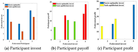
Figure 3. Comparison of investments and payoffs.

In Figure 3b, we can see that the participants who satisfy the Pareto optimal investments receive higher payoffs than the participants who satisfy the Nash equilibrium investments, while Figure 3c shows that federated participants receive higher maximum profits in the case of satisfying Pareto optimal investments than in the case of satisfying Nash equilibrium investments.

In Table 3, refs. [9,19,27,28] do not take ambiguity and Pareto optimality into account, although they do take fairness into account. In particular, ref. [27] only considers the fairness of the distribution of gains under participant attitude certainty and does not discuss in depth the issue of Pareto optimality in FL, which maximizes the gains for all participants. Meanwhile, ref. [29] considers the fairness and Pareto optimality of benefit distribution in the case of certainty of participants’ attitudes. Therefore, the method in this paper is more consistent with the practical application scenario, and it can solve the fairness and Pareto optimal consistency of gain distribution under uncertainty of participants’ attitudes, which can motivate more participants to join in the FL.

Table 3. Comparison of experimental results.

Research Methods	Fuzziness	Fairness	Pareto Optimality
[9,19,27,28]	✗	✓	✗
[29]	✗	✓	✓
This paper	✓	✓	✓

With these experimental simulation results, we can conclude that for FL, the investment strategy without the introduction of the monitoring mechanism does not reach the Nash equilibrium, and the investment strategy with the addition of the monitoring mechanism reaches the Pareto optimality.

6. Discussions

Constructing a fuzzy Shapley value technique that can manage the ambiguity in the uncertainty of participation attitudes in FL is achievable, and the extent of participants’ contributions and benefits can be assessed more accurately and through the introduction of a supervised mechanism. The method, through its mechanism, guarantees that the distribution of benefits is equitable and Pareto-efficient, which enhances the accuracy of the distribution of benefits.

However, the incentive mechanism also has some disadvantages: it involves several concepts and techniques such as fuzzy sets, fuzzy probabilities and supervision mechanisms, which increases the complexity of the mechanism, and the application of the mechanism to a real FL scenario needs to consider how to obtain and process information about the attitudes of participants towards participation and how to design and implement the supervision mechanism. In addition, there may be a degree of subjectivity in developing rules and standards for the supervised mechanism.

Therefore, the method has some advantages in dealing with the uncertainty of participants’ participation attitudes and achieving fairness and Pareto efficiency consistency in FL. At the same time, it also brings disadvantages to FL in its application, such as complexity, difficulty of implementation, and subjectivity of rule-making.

7. Conclusions

In the model training of FL, we considered the case of uncertain and ambiguous attitudes toward federated participant engagement, i.e., participants are not necessarily fully engaged in FL. To promote engagement among all participants in federated model training, this paper devises an incentive system utilizing the fuzzy Shapley value approach alongside supervised functions, which resolves the tension between equity and effectiveness in the distribution of payoffs within the FL. By conducting numerical computation validation and contrasting research findings, this paper constructs a fuzzy Shapley value method with supervised functions that helps to improve the effectiveness of FL, ensures the fairness and reasonableness of the participants in the distribution of payoffs.

Consequently, using this incentive mechanism guarantees the fairness of the distribution of benefits and the Pareto optimal consistency of the federated participants in the case of uncertainty and ambiguity in their attitude to participation, which offers theoretical insights for practical implementations.

Appendix A.1. Proof of Theorem 1

Proof. 

The validity of the traditional Shapley value implies that

$$\begin{array}{cc}\hfill \sum _{i=1}^n{\tilde{\phi }}_i(\tilde{v})& =\sum _{i=1}^n\sum _{l=1}^{q(S)}{\tilde{\phi }}_i(v({\left[S\right]}_{f_l}))(f_l-f_{l-1})\hfill \\ \hfill & =\sum _{l=1}^{q(S)}\sum _{i=1}^n{\tilde{\phi }}_i(v({\left[S\right]}_{f_l}))(f_l-f_{l-1})\hfill \\ \hfill & =\sum _{l=1}^{q(S)}v({\left[N\right]}_{f_l})(f_l-f_{l-1})\hfill \\ \hfill & =\tilde{v}(N)\hfill \end{array}$$

Hence, the validity of fuzzy Shapley value is established. □

Appendix A.2. Proof of Theorem 2

Proof. 

From the symmetry of classical Shapley values it follows that

$$\begin{array}{cc}\hfill \tilde{v}(S\cup \left\{i\right\})& =\sum _{l=1}^{q(S)}v({[S\cup \left\{i\right\}]}_{f_l})(f_l-f_{l-1}),\hfill \\ \hfill \tilde{v}(S\cup \left\{j\right\})& =\sum _{l=1}^{q(S)}v({[S\cup \left\{j\right\}]}_{f_l})(f_l-f_{l-1}),\hfill \\ \hfill {\tilde{\phi }}_i(\tilde{v})& =\sum _{l=1}^{q(S)}{\tilde{\phi }}_i(v({[S\cup \left\{i\right\}]}_{f_l}))(f_l-f_{l-1}),\hfill \\ \hfill {\tilde{\phi }}_j(\tilde{v})& =\sum _{l=1}^{q(S)}{\tilde{\phi }}_j(v({[S\cup \left\{j\right\}]}_{f_l}))(f_l-f_{l-1}),\hfill \end{array}$$

due to the fact that $\tilde{v}(S\cup \left\{i\right\})=\tilde{v}(S\cup \left\{j\right\})$, then

$$\begin{array}{cc}\hfill \sum _{l=1}^{q(S)}{\tilde{\phi }}_i(v({[S\cup \left\{i\right\}]}_{f_l}))(f_l-f_{l-1})& =\sum _{l=1}^{q(S)}{\tilde{\phi }}_j(v({[S\cup \left\{j\right\}]}_{f_l}))(f_l-f_{l-1})\hfill \end{array}$$

and thus ${\tilde{\phi }}_i(\tilde{v})={\tilde{\phi }}_j(\tilde{v})$. Hence, the symmetry of fuzzy Shapley value is proved. □

Appendix A.3. Proof of Theorem 3

Proof. 

The validity of the traditional Shapley value implies that

$$\begin{array}{cc}\hfill \left({\tilde{v}}_1+{\tilde{v}}_2\right)(S)& =\sum _{l=1}^{q(S)}(v_1({\left[S\right]}_{f_l})+v_2({\left[S\right]}_{f_l}))(f_l-f_{l-1})\hfill \\ \hfill & =\sum _{l=1}^{q(S)}{v}_1({\left[S\right]}_{f_l})(f_l-f_{l-1})+\sum _{l=1}^{q(S)}{v}_2({\left[S\right]}_{f_l})(f_l-f_{l-1})\hfill \\ \hfill & ={\tilde{v}}_1(S)+{\tilde{v}}_2(S)\hfill \end{array}$$

due to the fact that

$$\begin{array}{cc}\hfill {\tilde{\phi }}_i({\tilde{v}}_1+{\tilde{v}}_2)(S)& =\sum _{l=1}^{q(S)}{\tilde{\phi }}_i(v_1({\left[S\right]}_{f_l})+v_2({\left[S\right]}_{f_l}))(f_l-f_{l-1})\hfill \\ \hfill & =\sum _{l=1}^{q(S)}{\tilde{\phi }}_i(v_1({\left[S\right]}_{f_l}))(f_l-f_{l-1})+\sum _{l=1}^{q(S)}{\tilde{\phi }}_i(v_2({\left[S\right]}_{f_l}))(f_l-f_{l-1})\hfill \\ \hfill & ={\tilde{\phi }}_i\left({\tilde{v}}_1\right)+{\tilde{\phi }}_i\left({\tilde{v}}_2\right)\hfill \end{array}$$

and thus ${\tilde{\phi }}_i\left({\tilde{v}}_1+{\tilde{v}}_2\right)={\tilde{\phi }}_i\left({\tilde{v}}_1\right)+{\tilde{\phi }}_i\left({\tilde{v}}_2\right)$, hence the additivity of fuzzy Shapley value is proved. □

Appendix A.4. Proof of Theorem 4

Proof. 

From the dummy of classical Shapley value it follows that

$$\tilde{v}(S)=\sum _{l=1}^{q(S)}v({\left[S\right]}_{f_l})(f_l-f_{l-1}),$$

$$\tilde{v}(S\setminus \left\{i\right\})=\sum _{l=1}^{q(S)}v({[S\setminus \left\{i\right\}]}_{f_l})(f_l-f_{l-1})$$

due to the fact that $\tilde{v}(S)=\tilde{v}(S\setminus \left\{i\right\})$, hence

$$\begin{array}{c}\hfill \sum _{l=1}^{q(S)}v({\left[S\right]}_{f_l})(f_l-f_{l-1})=\sum _{l=1}^{q(S)}v({[S\setminus \left\{i\right\}]}_{f_l})(f_l-f_{l-1})\end{array}$$

and thus

$$\begin{array}{cc}\hfill {\tilde{\phi }}_i(\tilde{v})& =\sum _{l=1}^{q(S)}{\tilde{\phi }}_i(v({\left[S\right]}_{f_l}))(f_l-f_{l-1})\hfill \\ \hfill & =\sum _{l=1}^{q(S)}{\tilde{\phi }}_i(v({[S\setminus \left\{i\right\}]}_{f_l})(f_l-f_{l-1})\hfill \\ \hfill & =\sum _{l=1}^{q(S)}0(f_l-f_{l-1})\hfill \\ \hfill & =0\hfill \end{array}$$

Consequently, the dummy of fuzzy Shapley value is thus demonstrated. □

Appendix A.5. Proof of Theorem 5

Proof. 

With the legitimacy of the fuzzy Shapley value established, we can derive that

$$\sum _{i=1}^n{\tilde{\phi }}_i(\tilde{v}(x))=\tilde{v}(x),\forall \tilde{v}(x).$$

(A1)

By differentiating Formula (A1) with respect to x, we find that

$$\sum _{i=1}^n{{\tilde{\phi }}_i}^{\prime }(\tilde{v}(x))=1.$$

(A2)

Here, ${{\tilde{\phi }}_i}^{\prime }(\tilde{v}(x))=\partial {\tilde{\phi }}_i/\partial \tilde{v}(x)$ represents the partial derivative of ${\tilde{\phi }}_i$ with respect to $\tilde{v}(x)$. In the context of the Nash equilibrium, each federated participant’s investment is denoted as $x_i$, and their profit is given by ${\tilde{\pi }}_i(\tilde{v}(x))={\tilde{\phi }}_i(\tilde{v}(x))-{\tilde{c}}_i(x_i)$. The profit maximization for participant i occurs at:

$$max{\tilde{\pi }}_i(\tilde{v}(x))={\tilde{\phi }}_i(\tilde{v}(x))-{\tilde{c}}_i(x_i),i=1,2,\dots ,n$$

(A3)

The Nash equilibrium’s first-order condition is thus

$${\tilde{\phi }}_i^{\prime }(\tilde{v}(x))={\tilde{c}}_i^{\prime }(x),i=1,2,\dots ,n.$$

(A4)

where ${\tilde{\phi }}_i^{\prime }(\tilde{v}(x))=\partial {\tilde{\phi }}_i/\partial x$, $x_i^{\prime }=\partial \tilde{x}/\partial x_i$, ${\tilde{c}}_i^{\prime }(x)=\partial {\tilde{c}}_i(x)/\partial x_i$. To achieve maximum federated profits, federated investments must satisfy Pareto efficiency:

$$x^{*}=arg\underset{x}{max}\left(\tilde{v}(x)-\sum _{i=1}^n{\tilde{c}}_i\left(x_i\right)\right).$$

(A5)

The Pareto optimality’s first-order requirement is

$$x_i^{\prime }={\tilde{c}}_i^{\prime }(x),i=1,2,\dots ,n.$$

(A6)

By considering Formulas (A4) and (A6), we observe that the Nash equilibrium corresponds to Pareto optimality, requiring the fulfillment of the following conditions:

$${\tilde{\phi }}_i^{\prime }(\tilde{v}(x))=1,i=1,2,\dots ,n$$

(A7)

Yet, this is inconsistent with meeting the criterion of the fuzzy Shapley value requirement ${\displaystyle \sum _{i=1}^n}{\tilde{\phi }}_i^{\prime }(\tilde{v}(x))=1$. □

Appendix A.6. Proof of Theorem 6

Proof. 

For the discussion to be meaningful, let us suppose that when the federated participants attain Pareto efficiency, the allocated federal revenues according to the fuzzy Shapley value method for each participant i exceed their investment costs, i.e., $\tilde{v}(x_i^{*})>{\tilde{c}}_i(x_i^{*})$. If $x^{*}=(x_1^{*},x_2^{*},\dots ,x_n^{*})$ represents the Nash equilibrium of this mechanism, the following condition should hold: ${\tilde{\pi }}_i\left[\tilde{v}(x_i^{*},x_{n-i}^{*})\right]\ge {\tilde{\pi }}_i\left[\tilde{v}(x_i,x_{n-i}^{*})\right]$ and

$$\begin{array}{c}\hfill {\tilde{\phi }}_i(\tilde{v}(x^{*}))-{\tilde{c}}_i(x_i^{*})\ge {\tilde{\phi }}_i(\tilde{v}(x))-{\tilde{k}}_i-{\tilde{c}}_i(x_i)\\ \hfill {\tilde{k}}_i\ge [{\tilde{\phi }}_i(\tilde{v}(x))-{\tilde{c}}_i(x_i)]-[{\phi }_i(\tilde{v}(x^{*}))-{\tilde{c}}_i(x_i^{*})].\end{array}$$

(A8)

In the FL process, the coalition’s invisible and non-unique investment cost ${\tilde{c}}_i(x_i)$ makes Formula (A8) unsuitable for formulating penalties. However, it is important to note that ${\tilde{c}}_i(x_i)\ge 0$, leading to ${\tilde{\phi }}_i(\tilde{v}(x))-[{\tilde{\phi }}_i(\tilde{v}(x^{*}))-{\tilde{c}}_i(x_i^{*})]\ge [{\tilde{\phi }}_i(\tilde{v}(x))-{\tilde{c}}_i(x_i)]-[{\phi }_i(\tilde{v}(x^{*}))-{\tilde{c}}_i(x_i^{*})]$. Hence, Equation (A8) holds true solely under the condition that ${\tilde{k}}_i\ge {\tilde{\phi }}_i(\tilde{v}(x))-[{\phi }_i(\tilde{v}(x^{*}))-{\tilde{c}}_i(x_i^{*})]$, guaranteeing the realization of Pareto efficiency. Therefore, the penalty requirement for the overseer to achieve Pareto efficiency is

$${\tilde{k}}_i\ge {\tilde{\phi }}_i(\tilde{v}(x))-[{\tilde{\phi }}_i(\tilde{v}(x^{*}))-{\tilde{c}}_i(x_i^{*})].$$

(A9)

To enhance participants’ enthusiasm, it is vital to ensure that penalties are not overly steep and comply with the principles of restricted involvement and restricted liability. Assuming that all participants in FL have limited liability, the penalty amount should not exceed the participant’s payoff. Hence, if a participant’s payoff is zero, no penalty is necessary. Consequently, based on Formula (19), we derive ${\tilde{\phi }}_i(\tilde{v}(x))-{\tilde{k}}_i\ge 0$, leading to the conclusion that

$${\tilde{k}}_i\le {\tilde{\phi }}_i(\tilde{v}(x)).$$

(A10)

From Formulas (A9) and (A10), we establish the following expression:

$${\tilde{\phi }}_i(\tilde{v}(x))-[{\tilde{\phi }}_i(\tilde{v}(x^{*}))-{\tilde{c}}_i(x_i^{*})]\le {\tilde{k}}_i\le {\tilde{\phi }}_i(\tilde{v}(x)).$$

(A11)

If we denote the net gain of participant i following the penalty as ${\tilde{\delta }}_i$, then ${\tilde{\delta }}_i={\tilde{\phi }}_i(\tilde{v}(x))-{\tilde{k}}_i$. By utilizing Formula (A11), we obtain the following expression:

$$0\le {\tilde{\delta }}_i\le {\phi }_i(\tilde{v}(x^{*}))-{\tilde{c}}_i(x_i^{*})$$

(A12)

Building upon the earlier analysis and taking into account the constraint of restricted liability, the optimization of the Pareto value is accomplished. If the overseer’s penalty conforms to Equation (A11), the optimal mechanism can be delineated as:

$$\begin{array}{cc}{\tilde{r}}_i(x)=\left\{\begin{array}{c}{\tilde{\phi }}_i(\tilde{v}(x)),\\ {\tilde{\delta }}_i,\end{array}\right.\hfill & \begin{array}{c}\mathrm{if}\tilde{v}(x)\ge \tilde{v}(x^{*})\hfill \\ \mathrm{if}\tilde{v}(x)<v(x^{*})\hfill \end{array}\end{array}$$

(A13)

In this scenario, the value of ${\tilde{\delta }}_i$ must comply with Equation (A13), where $i=1,2,\dots ,n$. We will now proceed to explain the mechanism under two different penalty value conditions as specified in Formula (A13).

If ${\tilde{k}}_i={\tilde{\phi }}_i(\tilde{v}(x))$, it indicates that the overseer recognizes that the federated reward equals or exceeds the Pareto-efficient reward. Under such circumstances, the overseer will distribute the federated reward among all participants according to the equation of fuzzy Shapley value. Should the federated reward not reach the Pareto-efficient level, the entire will be affected by the overseer. The equation is as follows:

$$\begin{array}{cc}{\tilde{r}}_i(x)=\left\{\begin{array}{c}{\tilde{\phi }}_i(\tilde{v}(x)),\\ 0,\end{array}\right.\hfill & \begin{array}{c}\mathrm{if}\tilde{v}(x)\ge \tilde{v}(x^{*})\hfill \\ \mathrm{if}\tilde{v}(x)<v(x^{*}).\hfill \end{array}\end{array}$$

(A14)

Furthermore, we will illustrate that the federated investment $x^{*}=(x_1^{*},x_2^{*},\dots ,x_n^{*})$ leading to Pareto efficiency constitutes the Nash equilibrium of this mechanism. If we assume that participant i invests $x_i<x^{*}$ in the FL process, as the other participants allocate $x_{n-i}^{*}$, owing to the monotonic nature of the function $\tilde{v}(x)$, it follows that $\tilde{v}(x_i,x_{n-i}^{*})<\tilde{v}(x_i^{*},x_{n-i}^{*})$. Moreover, ${\tilde{r}}_i(x_i,x_{n-i}^{*})=0$, and participant i’s earnings amount to ${\tilde{\pi }}_i(x_i)=-{\tilde{c}}_i(x_i)\le 0$. Consequently, a rational participant i would not invest $x_i<x^{*}$. Given that participant i invests $x_i\ge x^{*}$ in the FL process, and considering the monotonicity of the function $\tilde{v}(x)$, the profit of participant i can be expressed as ${\tilde{\pi }}_i(x_i)={\tilde{\phi }}_i(x_i)-{\tilde{c}}_i(x_i)>0$. Consequently, a rational participant i would choose to invest $x_i\ge x^{*}$. □

References

- Konečnỳ, J.; McMahan, H.B.; Ramage, D.; Richtárik, P. Federated optimization: Distributed machine learning for on-device intelligence. arXiv 2016, arXiv:1610.02527. [Google Scholar]
- McMahan, H.B.; Moore, E.; Ramage, D.; y Arcas, B.A. Federated learning of deep networks using model averaging. arXiv 2016, arXiv:1602.05629. [Google Scholar]
- Konečnỳ, J.; McMahan, H.B.; Yu, F.X.; Richtárik, P.; Suresh, A.T.; Bacon, D. Federated learning: Strategies for improving communication efficiency. arXiv 2016, arXiv:1610.05492. [Google Scholar]
- Cicceri, G.; Tricomi, G.; Benomar, Z.; Longo, F.; Puliafito, A.; Merlino, G. Dilocc: An approach for distributed incremental learning across the computing continuum. In Proceedings of the 2021 IEEE International Conference on Smart Computing (SMARTCOMP), Irvine, CA, USA, 23–27 August 2021; pp. 113–120. [Google Scholar]
- Zhang, Z.; Zhang, Y.; Guo, D.; Zhao, S.; Zhu, X. Communication-efficient federated continual learning for distributed learning system with non-iid data. Sci. China Inf. Sci. 2023, 66, 122102. [Google Scholar] [CrossRef]
- Yang, Q.; Liu, Y.; Chen, T.; Tong, Y. Federated machine learning: Concept and applications. ACM Trans. Intell. Syst. Technol. (Tist) 2019, 10, 1–19. [Google Scholar] [CrossRef]
- Kairouz, P.; McMahan, H.B.; Avent, B.; Bellet, A.; Bennis, M.; Bhagoji, A.N.; Bonawitz, K.; Charles, Z.; Cormode, G.; Cummings, R.; et al. Advances and open problems in federated learning. Found. Trends Mach. Learn. 2021, 14, 1–210. [Google Scholar] [CrossRef]
- Sarikaya, Y.; Ercetin, O. Motivating workers in federated learning: A stackelberg game perspective. IEEE Netw. Lett. 2019, 2, 23–27. [Google Scholar] [CrossRef]
- Yu, H.; Liu, Z.; Liu, Y.; Chen, T.; Cong, M.; Weng, X.; Niyato, D.; Yang, Q. A fairness-aware incentive scheme for federated learning. In Proceedings of the Proceedings of the AAAI/ACM Conference on AI, Ethics, and Society, New York, NY, USA, 7–9 February 2020; Volume 2020, pp. 393–399. [Google Scholar]
- Li, T.; Sanjabi, M.; Beirami, A.; Smith, V. Fair resource allocation in federated learning. arXiv 2019, arXiv:1905.10497. [Google Scholar]
- Zhan, Y.; Li, P.; Qu, Z.; Zeng, D.; Guo, S. A learning-based incentive mechanism for federated learning. IEEE Internet Things J. 2020, 7, 6360–6368. [Google Scholar] [CrossRef]
- Kang, J.; Xiong, Z.; Niyato, D.; Xie, S.; Zhang, J. Incentive mechanism for reliable federated learning: A joint optimization approach to combining reputation and contract theory. IEEE Internet Things J. 2019, 6, 10700–10714. [Google Scholar] [CrossRef]
- Tran, N.H.; Bao, W.; Zomaya, A.; Nguyen, M.N.; Hong, C.S. Federated learning over wireless networks: Optimization model design and analysis. In Proceedings of the IEEE INFOCOM 2019-IEEE conference on computer communications, Paris, France, 29 April–2 May 2019; pp. 1387–1395. [Google Scholar]
- Kim, H.; Park, J.; Bennis, M.; Kim, S.L. Blockchained on-device federated learning. IEEE Commun. Lett. 2019, 24, 1279–1283. [Google Scholar] [CrossRef]
- Feng, S.; Niyato, D.; Wang, P.; Kim, D.I.; Liang, Y.C. Joint service pricing and cooperative relay communication for federated learning. In Proceedings of the 2019 International Conference on Internet of Things (iThings) and IEEE Green Computing and Communications (GreenCom) and IEEE Cyber, Physical and Social Computing (CPSCom) and IEEE Smart Data (SmartData), Atlanta, GA, USA, 14–17 July 2019; pp. 815–820. [Google Scholar]
- Yang, X. An exterior point method for computing points that satisfy second-order necessary conditions for a C1, 1 optimization problem. J. Math. Anal. Appl. 1994, 187, 118–133. [Google Scholar] [CrossRef]
- Wang, Z.; Hu, Q.; Li, R.; Xu, M.; Xiong, Z. Incentive mechanism design for joint resource allocation in blockchain-based federated learning. IEEE Trans. Parallel Distrib. Syst. 2023, 34, 1536–1547. [Google Scholar] [CrossRef]
- Song, T.; Tong, Y.; Wei, S. Profit allocation for federated learning. In Proceedings of the 2019 IEEE International Conference on Big Data (Big Data), Los Angeles, CA, USA, 9–12 December 2019; pp. 2577–2586. [Google Scholar]
- Wang, T.; Rausch, J.; Zhang, C.; Jia, R.; Song, D. A principled approach to data valuation for federated learning. In Federated Learning: Privacy and Incentive; Springer: Berlin/Heidelberg, Germany, 2020; pp. 153–167. [Google Scholar]
- Wang, G.; Dang, C.X.; Zhou, Z. Measure contribution of participants in federated learning. In Proceedings of the 2019 IEEE international conference on big data (Big Data), Los Angeles, CA, USA, 9–12 December 2019; pp. 2597–2604. [Google Scholar]
- Liu, Y.; Ai, Z.; Sun, S.; Zhang, S.; Liu, Z.; Yu, H. Fedcoin: A peer-to-peer payment system for federated learning. In Federated Learning: Privacy and Incentive; Springer: Berlin/Heidelberg, Germany, 2020; pp. 125–138. [Google Scholar]
- Zeng, R.; Zeng, C.; Wang, X.; Li, B.; Chu, X. A comprehensive survey of incentive mechanism for federated learning. arXiv 2021, arXiv:2106.15406. [Google Scholar]
- Liu, Z.; Chen, Y.; Yu, H.; Liu, Y.; Cui, L. Gtg-shapley: Efficient and accurate participant contribution evaluation in federated learning. ACM Trans. Intell. Syst. Technol. (Tist) 2022, 13, 1–21. [Google Scholar] [CrossRef]
- Nagalapatti, L.; Narayanam, R. Game of gradients: Mitigating irrelevant clients in federated learning. Proc. AAAI Conf. Artif. Intell. 2021, 35, 9046–9054. [Google Scholar] [CrossRef]
- Fan, Z.; Fang, H.; Zhou, Z.; Pei, J.; Friedlander, M.P.; Liu, C.; Zhang, Y. Improving fairness for data valuation in horizontal federated learning. In Proceedings of the 2022 IEEE 38th International Conference on Data Engineering (ICDE), Kuala Lumpur, Malaysia, 9–12 May 2022; pp. 2440–2453. [Google Scholar]
- Fan, Z.; Fang, H.; Zhou, Z.; Pei, J.; Friedlander, M.P.; Zhang, Y. Fair and efficient contribution valuation for vertical federated learning. arXiv 2022, arXiv:2201.02658. [Google Scholar]
- Yang, X.; Tan, W.; Peng, C.; Xiang, S.; Niu, K. Federated Learning Incentive Mechanism Design via Enhanced Shapley Value Method. Wirel. Commun. Mob. Comput. 2022, 2022, 9690657. [Google Scholar] [CrossRef]
- Pene, P.; Liao, W.; Yu, W. Incentive Design for Heterogeneous Client Selection: A Robust Federated Learning Approach. IEEE Internet Things J. 2023, 11, 5939–5950. [Google Scholar] [CrossRef]
- Yang, X.; Xiang, S.; Peng, C.; Tan, W.; Li, Z.; Wu, N.; Zhou, Y. Federated Learning Incentive Mechanism Design via Shapley Value and Pareto Optimality. Axioms 2023, 12, 636. [Google Scholar] [CrossRef]
- McMahan, B.; Moore, E.; Ramage, D.; Hampson, S.; y Arcas, B.A. Communication-efficient learning of deep networks from decentralized data. In Proceedings of the Artificial Intelligence and Statistics. PMLR, Fort Lauderdale, FL, USA, 20–22 April 2017; pp. 1273–1282. [Google Scholar]
- Shapley, L.S. A value for n-person games. Contrib. Theory Games 1953, 2, 307–317. [Google Scholar]
- Murofushi, T.; Sugeno, M. An interpretation of fuzzy measures and the Choquet integral as an integral with respect to a fuzzy measure. Fuzzy Sets Syst. 1989, 29, 201–227. [Google Scholar] [CrossRef]
- Mesiar, R. Fuzzy measures and integrals. Fuzzy Sets Syst. 2005, 156, 365–370. [Google Scholar] [CrossRef]
- Zhou, Z.H.; Yu, Y.; Qian, C. Evolutionary Learning: Advances in Theories and Algorithms; Springer: Berlin/Heidelberg, Germany, 2019. [Google Scholar]
- Pardalos, P.M.; Migdalas, A.; Pitsoulis, L. Pareto Optimality, Game Theory and Equilibria; Springer Science & Business Media: Berlin/Heidelberg, Germany, 2008; Volume 7. [Google Scholar]
- Nas, J. Non-cooperative games. Ann. Math. 1951, 54, 286–295. [Google Scholar] [CrossRef]
- Ye, M.; Hu, G. Distributed Nash Equilibrium Seeking by a Consensus Based Approach. IEEE Trans. Autom. Control 2017, 62, 4811–4818. [Google Scholar] [CrossRef]
- Kang, J.; Xiong, Z.; Niyato, D.; Yu, H.; Liang, Y.C.; Kim, D.I. Incentive design for efficient federated learning in mobile networks: A contract theory approach. In Proceedings of the 2019 IEEE VTS Asia Pacific Wireless Communications Symposium (APWCS), Singapore, 28–30 August 2019; pp. 1–5. [Google Scholar]
- Pandey, S.R.; Tran, N.H.; Bennis, M.; Tun, Y.K.; Manzoor, A.; Hong, C.S. A crowdsourcing framework for on-device federated learning. IEEE Trans. Wirel. Commun. 2019, 19, 3241–3256. [Google Scholar] [CrossRef]
- Deng, J.; Guo, J.; Zafeiriou, S. Arcface: Additive angular margin loss for deep face recognition. In Proceedings of the IEEE/CVF Conference on Computer Vision and Pattern Recognition, Long Beach, CA, USA, 15–20 June 2019; pp. 4690–4699. [Google Scholar]
- De Boer, P.T.; Kroese, D.P.; Mannor, S.; Rubinstein, R.Y. A tutorial on the cross-entropy method. Ann. Oper. Res. 2005, 134, 19–67. [Google Scholar] [CrossRef]
- Jauernig, P.; Sadeghi, A.R.; Stapf, E. Trusted execution environments: Properties, applications, and challenges. IEEE Secur. Priv. Mag. 2020, 8, 56–60. [Google Scholar] [CrossRef]
- Wang, H.; Kaplan, Z.; Niu, D.; Li, B. Optimizing federated learning on non-iid data with reinforcement learning. In Proceedings of the IEEE INFOCOM 2020-IEEE Conference on Computer Communications, Toronto, ON, Canada, 6–9 July 2020; pp. 1698–1707. [Google Scholar]
- Karimireddy, S.P.; Kale, S.; Mohri, M.; Reddi, S.; Stich, S.; Suresh, A.T. Scaffold: Stochastic controlled averaging for federated learning. Int. Conf. Mach. Learn. 2019, 119, 5132–5143. [Google Scholar]
- Alchian, A.A.; Demsetz, H. Production, information costs, and economic organization. Am. Econ. Rev. 1972, 62, 777–795. [Google Scholar]
- Holmstrom, B. Moral hazard in teams. Bell J. Econ. 1982, 13, 324–340. [Google Scholar] [CrossRef]
Disclaimer/Publisher’s Note: The statements, opinions and data contained in all publications are solely those of the individual author(s) and contributor(s) and not of MDPI and/or the editor(s). MDPI and/or the editor(s) disclaim responsibility for any injury to people or property resulting from any ideas, methods, instructions or products referred to in the content. |
© 2024 by the authors. Licensee MDPI, Basel, Switzerland. This article is an open access article distributed under the terms and conditions of the Creative Commons Attribution (CC BY) license (https://creativecommons.org/licenses/by/4.0/).