Strict Vector Equilibrium Problems of Multi-Product Supply–Demand Networks with Capacity Constraints and Uncertain Demands

Abstract

This paper considers a multi-product, multi-criteria supply–demand network equilibrium model with capacity constraints and uncertain demands. Strict network equilibrium principles are proposed both in the case of a single criterion and multi-criteria, respectively. Based on a single criterion, it proves that strict network equilibrium flows are equivalent to vector variational inequalities, and the existence of strict network equilibrium flows is derived by virtue of the Fan–Browder fixed point theorem. Based on multi-criteria, the scalarization of strict network equilibrium flows is given by using Gerstewitz’s function without any convexity assumptions. Meanwhile, the necessary and sufficient conditions of strict network equilibrium flows are derived in terms of vector variational inequalities. Finally, an example is given to illustrate the application of the derived theoretical results.

1. Introduction

The study of the supply–demand network equilibrium models has been the subject of great interest due to their theoretical challenges and practical application. The fundamental principle is Wardrop’s equilibrium principle [1], which states that users in transport networks choose one of the paths among all the paths joining the same origin–destination (OD) pair at minimum cost. After Wardrop, many scholars have proposed various network equilibrium models based on a single criterion. Dong et al. [2] considered a supply chain network equilibrium model with random demands. Meng et al. [3] proposed a note on supply chain network equilibrium models. Nagurney [4] presented a supply chain network equilibrium model and investigated the relationship between transportation and supply chain network equilibria. Nagurney et al. [5] developed an equilibrium model of a competitive supply chain network. Additionally, motivated by practical concerns, network equilibrium models based on multiple criteria cost functions have been studied; for example, Chen and Yen [6] were the first to propose a traffic network equilibrium model based on multiple criteria cost functions without capacity constraints, and present an equivalent relation between vector network equilibrium models and vector variational inequalities. Cheng and Wu [7] presented a multi-product supply–demand network equilibrium model with multiple criteria.

For a supply–demand network, it is well known that when the flows pass through two different paths which contain common arcs at the same time, the capacity constraints of the two paths may interact. So, the capacity constraints are important factors that affect the equilibrium states and the selection of the set of feasible network flows. Based on this cause, a substantial number of works have been devoted to studying the vector equilibrium principle [5,8,9,10,11,12,13,14] with capacity constraints of paths. In addition, considering that the data are uncertain in practice and are not known exactly, along with the change of network users’ demand preferences and the fluctuation of purchasing power, the demands of network flow should not be fixed, and the network equilibrium with uncertain demands have attracted much attention. Very recently, Cao et al. [15] focused on the traffic network equilibrium problem with uncertain demands, in which the uncertain set consisted of finite discrete scenarios. Subsequently, Wei et al. [16] assumed that the demands belonged to a closed interval and proposed (weak) vector equilibrium principles involving a single product. Proper efficiency is widely applied to solve vector optimization and vector equilibrium problems. It can help one to eliminate some abnormal efficient decisions and provide proper efficient decisions. Several classical proper efficiency measures, such as Benson efficiency [17], super efficiency [18], and Henig efficiency [19], have been applied to solve network equilibrium models. Cheng and Fu [20] introduced a kind of proper efficiency–strict efficiency, and it has been used to solve vector optimization models (for example, see Yu et al. [21]). On the other hand, variational inequality theory is an effective tool to solve equilibrium problems (for example, see Chen and Yen [6]).

In this paper, inspired by the work in [7,10,16,17], we consider strict vector equilibrium principles of a multi-product, multi-criteria supply–demand network with capacity constraints and uncertain demands, where the demands are assumed to belong to a closed interval and are irrelevant to the costs for all OD pairs. The main contribution is to derive the existence results of strict vector equilibrium flows of a multi-product supply–demand network with capacity constraints and uncertain demands by virtue of the Fan–Browder fixed point theorem and obtain the relations between the strict vector equilibrium flows and vector variational inequalities, with both a single criterion and multi-criteria cost functions, which, to the best of our knowledge have not been studied before.

The rest of this article is arranged as follows: in Section 2, some mathematical preliminaries are described. In Section 3, we propose a strict network equilibrium principle for a multi-product supply–demand network problem involving real-valued cost functions with capacity constraints and uncertain demands. The equivalence relation between the strict network equilibrium flow and the strictly efficient solution of variational inequalities is established. The existence of the strict network equilibrium flows is also derived by means of the Fan–Browder fixed point theorem. Section 4 proposes a strict network equilibrium principle for a multi-product supply–demand network problem with capacity constraints and uncertain demands involving vector-valued cost functions, and the similar equivalence relation of strict network equilibrium flows in terms of vector variational inequalities is deduced by using Gerstewitz’s scalarization function. Section 5 gives an illustrative example. Section 6 provides a brief summary of the paper.

2. Definition and Preliminaries

In this section, some notations are set and we recall the notions of efficient points of a nonempty set, and the variational inequality and strictly efficient points of a nonempty set. Throughout the paper, we suppose that the vectors are always row vectors unless otherwise stated. Let ${\mathbb{R}}^n$ be the n-dimensional Euclidean space and ${\mathbb{R}}_{+}^n$ be its non-negative orthant. Let ${\mathbb{R}}^{n\times n}$ be the $n\times n$ matrix space and

$${\mathbb{R}}_{+}^{n\times n}=\{k=(k_1,\cdots ,k_n)\in {\mathbb{R}}^{n\times n}:k_i={(k_i^1,\cdots ,k_i^n)}^{\prime },k_i^j\ge 0,j=1,\cdots ,n\}$$

be its non-negative orthant, where ${(k_i^1,\cdots ,k_i^n)}^{\prime }$ denotes the transpose of the matrix $(k_i^1,\cdots ,k_i^n)$. Given $y,z\in {\mathbb{R}}^{n\times n}$, let $\langle y,z^{\prime }\rangle =y{z}^{\prime }$ represent the multiplication of matrix y and z. A pointed closed convex cone $\Gamma \subset {\mathbb{R}}^n$ induces the orderings in ${\mathbb{R}}^n$: for any $x_1,x_2\in {\mathbb{R}}^n$,

$$\begin{array}{c}\hfill x_1⩽x_2\mathrm{iff}{x}_2-x_1\in \Gamma ,\\ \hfill x_1<x_2\mathrm{iff}{x}_2-x_1\in \mathrm{int}\Gamma ,\end{array}$$

where $\mathrm{int}\Gamma$ denotes the nonempty interior of $\Gamma$. For convenience of writing, let ${\mathbb{R}}^n=X$. Let ${\Xi }_X$ be a nonempty convex subset of the cone $\Gamma$ and $\mathrm{cl}\left({\Xi }_X\right)$ be its closure. $\mathrm{cone}\left({\Xi }_X\right)=\{\sigma x:\sigma \in R_{+}^1,x\in {\Xi }_X\}$ is the conic hull of the set ${\Xi }_X$. If $0\notin \mathrm{cl}\left({\Xi }_X\right)$, $\Gamma =\mathrm{cone}\left({\Xi }_X\right)$, then the set ${\Xi }_X$ is said to be a base of the cone $\Gamma$.

Let N be a nonempty subset of X; $H:N\to {\mathbb{R}}^n$ is a mapping. The notion of efficient points of the set N is as follows.

Definition 1

(see [21]). A vector $\overline{x}\in N$ is said to be an efficient point of the set N if

$$\begin{array}{c}\hfill (N-\overline{x})\cap (-\Gamma \setminus \left\{0\right\})=\varnothing .\end{array}$$

Let EP(N) denote the set of the efficient points of the set N.

The variational inequality is to find a vector $\overline{x}\in N$, such that

$$\langle H\left(\overline{x}\right),x-\overline{x}\rangle \ge 0,\forall x\in N.$$

The concept of strictly efficient points of the set N is as follows.

Definition 2

(see [21]). Suppose that ${\Xi }_X$ is a base of Γ. The vector $\overline{x}\in N$ is called a strictly efficient point of the set N with ${\Xi }_X$ if there is a neighborhood ${\Theta }_X$ of 0, such that

$$\mathit{cone}(N-\overline{x}+\Gamma )\cap ({\Theta }_X-{\Xi }_X)=\varnothing .$$

Let SEP(N) denote the set of strictly efficient points of the set N.

3. Existence of Strict Vector Equilibrium Flows with Single Criterion

For a supply–demand network $\mathcal{G}=[\mathcal{N},\mathcal{C},\mathcal{V},\mathcal{P},\mathcal{D}]$, let $\mathcal{N},\mathcal{C},\mathcal{P}$, and $\mathcal{D}$ denote the set of nodes, the set of arcs, the set of OD pairs, and the uncertain demand vectors, respectively. Let us suppose that there are m different kinds of products passing through the network and that a typical product is denoted by o. For each arc $c\in \mathcal{C}$ and product o, ${\varrho }_c^o$ represents arc flow of product o between two different nodes. $\mathcal{V}={\left({\overline{\varrho }}_c^o\right)}_{\in C}$ denotes the capacity vector, where ${\overline{\varrho }}_c^o>0$ implies the capacity of arc c for the product o. The arc flow ${\varrho }_c^o$ needs to satisfy the following capacity constraint:

$$0\le {\varrho }_c^o\le {\overline{\varrho }}_c^o.$$

Let us assume that there are s OD pairs in the set $\mathcal{P}$. The available paths connecting OD pair $p\in \mathcal{P}$ form the set ${\omega }_p$, and let ${\sum }_{p\in \mathcal{P}}\left|{\omega }_p\right|=n$, where n is a positive integer. For each acyclic path $a\in {\omega }_p$, we denote by ${\varrho }_a^o\ge 0$ the path flow of the product o on path a. The relation between arc flows and path flows is as follows:

$${\varrho }_c^o=\sum _{p\in \mathcal{P}}\sum _{a\in {\omega }_p}{\delta }_{ca}{\varrho }_a^o,$$

where

$${\delta }_{ca}=\left\{\begin{array}{cc}1,\hfill & ifcbelongstopatha,\hfill \\ 0,\hfill & otherwise.\hfill \end{array}\right.$$

Let us suppose that ${\mu }_a^o$ and ${\lambda }_a^o$ are the lower and upper capacity constraints on path a with product o, respectively, i.e.,

$${\mu }_a^o\le {\varrho }_a^o\le {\lambda }_a^o.$$

The matrix $\varrho ={\left({\varrho }_a^o\right)}_{m\times n}$ is called a network flow. Thus, each column vector ${\varrho }_a={({\varrho }_a^1,\cdots ,{\varrho }_a^m)}^{\prime }$ of the matrix $\varrho$ is the flow on path a, while the row vector ${\varrho }^o=({\varrho }_1^o,\cdots ,{\varrho }_n^o)$ is the network flow with product o.

We denote demand vectors of the network flow by $\mathcal{D}=(d_p^o\left({\epsilon }_p^o\right):p\in \mathcal{P},o=1,\cdots ,m)$, where the component $d_p^o\left({\epsilon }_p^o\right)$ denotes the uncertain demand for OD pair p and product o. Let us suppose that $d_p^o\left({\epsilon }_p^o\right)$ belongs to a closed interval ${\Delta }_p^o$, i.e., $d_p^o\left({\epsilon }_p^o\right)\in {\Delta }_p^o=[d_p^o-{\epsilon }_p^o,d_p^o+{\epsilon }_p^o]$, where $d_p^o$ represents an appropriate fixed demand and ${\epsilon }_p^o\ge 0$ denotes a deviation. It is reasonable to assume that the values of $d_p^o$ and ${\epsilon }_p^o$ that depend on p and o are different for each OD pair and product in practical supply–demand network problems. We would like to point out that the uncertain demand $d_p^o\left({\epsilon }_p^o\right)$ that is irrelevant to the costs is significantly different from the one introduced in [12,22].

We say that the network flow $\varrho$ satisfies the uncertain demands constraint if and only if

$$\sum _{a\in {\omega }_p}{\varrho }_a^o=d_p^o\left({\epsilon }_p^o\right),\forall p\in \mathcal{P},o=1,\cdots ,m.$$

A network flow $\varrho$ satisfying both the capacity constraints and the uncertain demands constraints is called a feasible flow. The set of all feasible flows is denoted by

$$Q=\{\varrho :{\mu }_a^o\le {\varrho }_a^o\le {\lambda }_a^o,0\le \sum _{p\in \mathcal{P}}\sum _{a\in {\omega }_p}{\delta }_{ca}{\varrho }_a^o\le {\overline{\varrho }}_c^o,\forall c\in \mathcal{C},\mathrm{and}$$

$$\sum _{a\in {\omega }_p}{\varrho }_a^o=d_p^o\left({\epsilon }_p^o\right),\forall p\in \mathcal{P},\forall o=1,\cdots ,m\}.$$

Let $Q\ne \varnothing$. Clearly, Q is closed, convex, and compact.

For each product o, let $h_c^o\left(\varrho \right):{\mathbb{R}}^{m\times n}\to {\mathbb{R}}_{+}$ be the cost function on arc c; the cost function on path $a\in {\omega }_p$ is computed by

$$h_a^o\left(\varrho \right)=\sum _{c\in a}{h}_c^o\left(\varrho \right).$$

The cost on the network is given as a form of matrix $h\left(\varrho \right)={\left(h_a^o\left(\varrho \right)\right)}_{m\times n}$, where the ath column $h_a\left(\varrho \right)={(h_a^1\left(\varrho \right),\cdots ,h_a^m\left(\varrho \right))}^{\prime }$ represents the cost on path a; the oth row $h^o\left(\varrho \right)=(h_1^o\left(\varrho \right),\cdots ,h_n^o\left(\varrho \right))$ represents the cost on the network with product o. In this paper, unless otherwise stated, we always assume that for any $p\in \mathcal{P}$ and $a,b\in {\omega }_p$,

$$h_b\left(\varrho \right)-h_a\left(\varrho \right)\ne 0,\mathrm{if}b\ne a,$$

which has been also used in the literature [7].

Definition 3.

Supposing a flow $\varrho \in Q$,

(i) 

 for an arc $c\in \mathcal{C}$ and product $o=1,\cdots ,m$, if ${\varrho }_c^o={\overline{\varrho }}_c^o$, then c is called a saturated arc of product o and flow ϱ, or a nonsaturated arc of product o and flow ϱ.

(ii) 

for a path $a\in {\bigcup }_{p\in \mathcal{P}}{\omega }_p$ and product $o=1,\cdots ,m$, if the path a contains a saturated arc c of product o and flow ϱ, then a is called a saturated path of product o and flow ϱ, otherwise, a nonsaturated path of product o and flow ϱ.

In the following content, we propose the concept of strict network equilibrium flow for a kind of multi-product supply–demand network involving real-valued cost functions with capacity constraints and uncertain demands, which has not been studied in the existing literature. In what follows, we always assume that $\Xi$ is a base of ${\mathbb{R}}_{+}^m$, $\tilde{\Xi }$ is a base of ${\mathbb{R}}_{+}^{m\times m}$, $\Theta$ is a neighborhood of 0 in ${\mathbb{R}}^m$, and $\tilde{\Theta }$ is a neighborhood of 0 in ${\mathbb{R}}^{m\times m}$.

Definition 4.

(Strict network equilibrium principle). A feasible network flow $\varrho \in Q$ is a strict network equilibrium flow, if, for each $p\in \mathcal{P}$, $a,b\in {\omega }_p$, $o=1,\cdots ,m$, there is a neighborhood Θ of 0 in ${\mathbb{R}}^m$ satisfying $\Theta -\Xi \subset -\mathit{int}{\mathbb{R}}_{+}^m$, one has as an implication

$$\begin{array}{c}\hfill \mathit{cone}(h_{{\omega }_p}\left(\varrho \right)+{\mathbb{R}}_{+}^m-h_a\left(\varrho \right))\cap (\mathit{cone}(\Theta -\Xi )\setminus \left\{0\right\})=\varnothing \\ \hfill h_b\left(\varrho \right)-h_a\left(\varrho \right)\ne 0\end{array}\}\Rightarrow$$

${\varrho }_b^o={\mu }_b^o$, $b\ne a$, or ${\varrho }_a^o={\lambda }_a^o$, or path a is a saturated path with product o and flow ϱ.

Now, let us review the concept of the strict efficiency of vector variational inequalities, which will be employed to derive the main conclusions.

Definition 5.

A flow $\varrho \in Q$ is said to be a strictly efficient solution of the vector variational inequality if and only if there exist $\tilde{\Xi }$ and $\tilde{\Theta }$ satisfying $\tilde{\Theta }-\tilde{\Xi }\subset -\mathit{int}{\mathbb{R}}_{+}^{m\times m}$,

$$\mathit{cone}(\langle h\left(\varrho \right),{(\chi -\varrho )}^{\prime }\rangle +{\mathbb{R}}_{+}^{m\times m})\cap (\mathit{cone}(\tilde{\Theta }-\tilde{\Xi })\setminus \left\{0\right\})=\varnothing ,\forall \chi \in Q.$$

It is noteworthy that the vector $\varrho \in Q$ is a strictly efficient solution of the following variational inequality:

$$\mathrm{cone}(\langle h\left(\varrho \right),{(\chi -\varrho )}^{\prime }\rangle +{\mathbb{R}}_{+}^{m\times m})\cap (\mathrm{cone}(\tilde{\Theta }-\tilde{\Xi })\setminus \left\{0\right\})=\varnothing ,\forall \chi \in Q,$$

if the vector $\varrho \in Q$ is a solution of the following variational inequality: find $\varrho \in Q$, satisfying

$$\langle h\left(\varrho \right),{(\chi -\varrho )}^{\prime }\rangle \notin -{\mathbb{R}}_{+}^{m\times m}\setminus \left\{0\right\},\forall \chi \in Q,$$

Next, we shall consider the relations between a strictly efficient solution of the vector variational inequality and the strict network equilibrium flow.

Theorem 1.

If the vector $\varrho \in Q$ is a strict network equilibrium flow, then ϱ is a strictly efficient solution of the following variational inequality: find $\varrho \in Q$, satisfying

$$\mathit{cone}(\langle h\left(\varrho \right),{(\chi -\varrho )}^{\prime }\rangle +{\mathbb{R}}_{+}^{m\times m})\cap (\mathit{cone}(\tilde{\Theta }-\tilde{\Xi })\setminus \left\{0\right\})=\varnothing ,\forall \chi \in Q.$$

Proof. 

If the vector $\varrho \in Q$ is a strict network equilibrium flow, for each $p\in \mathcal{P}$, $a,b\in {\omega }_p$, $o=1,\cdots ,m$, it has the following implication:

$$\begin{array}{c}\hfill \mathrm{cone}(h_{{\omega }_p}\left(\varrho \right)+{\mathbb{R}}_{+}^m-h_a\left(\varrho \right))\cap (\mathrm{cone}(\Theta -\Xi )\setminus \left\{0\right\})=\varnothing \\ \hfill h_b\left(\varrho \right)-h_a\left(\varrho \right)\ne 0\end{array}\}\Rightarrow$$

${\varrho }_b^o={\mu }_b^o$, $b\ne a$, or ${\varrho }_a^o={\lambda }_a^o$, or path a is a saturated path of product o and flow $\varrho$.

We first show that

$$\langle h\left(\varrho \right),{(\chi -\varrho )}^{\prime }\rangle \notin -{\mathbb{R}}_{+}^{m\times m},\forall \chi \in Q.$$

(1)

For any $\chi \in Q$, it holds

$$\begin{array}{ccc}& & \langle h\left(\varrho \right),{(\chi -\varrho )}^{\prime }\rangle \hfill \\ & & =\langle (h_1\left(\varrho \right),\cdots ,h_n\left(\varrho \right)),{({\chi }_1-{\varrho }_1,\cdots ,{\chi }_n-{\varrho }_n)}^{\prime }\rangle \hfill \\ & & =\sum _{\overline{a}=1}^n\langle h_{\overline{a}}\left(\varrho \right),{({\chi }_{\overline{a}}-{\varrho }_{\overline{a}})}^{\prime }\rangle \hfill \\ & & =\sum _{p=1}^s\left[\sum _{\overline{a}\in {\omega }_p}\langle h_{\overline{a}}\left(\varrho \right),{({\chi }_{\overline{a}}-{\varrho }_{\overline{a}})}^{\prime }\rangle \right].\hfill \end{array}$$

Because $\langle h_{\overline{a}}\left(\varrho \right),{({\chi }_{\overline{a}}-{\varrho }_{\overline{a}})}^{\prime }\rangle$ is an $m\times m$ matrix, the component is $h_{\overline{a}}^{\rho }\left(\varrho \right)({\chi }_{\overline{a}}^{\eta }-{\varrho }_{\overline{a}}^{\eta })$, $\rho ,\eta =1,2,\cdots ,m$; so, $\langle h\left(\varrho \right),{(\chi -\varrho )}^{\prime }\rangle$ is also an $m\times m$ matrix, the component is ${\sum }_{p=1}^s\left[{\sum }_{\overline{a}\in {\omega }_p}{h}_{\overline{a}}^{\rho }\left(\varrho \right)({\chi }_{\overline{a}}^{\eta }-{\varrho }_{\overline{a}}^{\eta })\right]$, $\rho ,\eta =1,2,\cdots ,m$. Let

$${\wedge }_p\left(\varrho \right)=\{\overline{b}\in {\omega }_p:h_{\overline{b}}\left(\varrho \right)\in \mathrm{SEP}\{h_b\left(\varrho \right):b\in {\omega }_p\}\}\subset {\omega }_p.$$

Hence, for each $\overline{b}\in {\wedge }_p\left(\varrho \right)\subset {\omega }_p$,

$$\mathrm{cone}(h_{{\omega }_p}\left(\varrho \right)+{\mathbb{R}}_{+}^m-h_{\overline{b}}\left(\varrho \right))\cap (\mathrm{cone}(\Theta -\Xi )\setminus \left\{0\right\})=\varnothing .$$

It follows from Definition 4 that for any $b\in {\omega }_p$, $o=1,\cdots ,m$ and $b\ne \overline{b}$, ${\varrho }_b^o={\mu }_b^o$, ${\varrho }_{\overline{b}}^o={\lambda }_{\overline{b}}^o$, or path $\overline{b}$ is a saturated path of product o and flow $\varrho$. Because $\mathrm{SEP}\{h_b\left(\varrho \right):b\in {\omega }_p\}\subset \mathrm{EP}\{h_b\left(\varrho \right):b\in {\omega }_p\}$, we obtain

$$h_{\overline{b}}\left(\varrho \right)\in \mathrm{EP}\{h_b\left(\varrho \right):b\in {\omega }_p\},$$

that is,

$$h_b\left(\varrho \right)-h_{\overline{b}}\left(\varrho \right)\notin -{\mathbb{R}}_{+}^m\setminus \left\{0\right\},\forall b\in {\omega }_p,p\in \mathcal{P} \mathrm{a}\mathrm{n}\mathrm{d} b\ne \overline{b}.$$

Due to $h_b\left(\varrho \right)-h_{\overline{b}}\left(\varrho \right)\ne 0$, one has

$$h_b\left(\varrho \right)-h_{\overline{b}}\left(\varrho \right)\notin -{\mathbb{R}}_{+}^m,\forall b\in {\omega }_p,p\in \mathcal{P} \mathrm{a}\mathrm{n}\mathrm{d} b\ne \overline{b}.$$

So there is an $\overline{\rho }=1,2,\cdots ,m$ such that

$$h_b^{\overline{\rho }}\left(\varrho \right)-h_{\overline{b}}^{\overline{\rho }}\left(\varrho \right)>0.$$

Hence, one has

$$\begin{array}{ccc}& & \sum _{p=1}^s\left[\sum _{\overline{a}\in {\omega }_p}{h}_{\overline{a}}^{\overline{\rho }}\left(\varrho \right)({\chi }_{\overline{a}}^{\eta }-{\varrho }_{\overline{a}}^{\eta })\right]\hfill \\ & & =\sum _{p=1}^s\left[\sum _{\overline{a}\in {\omega }_p\setminus \left\{\overline{b}\right\}}{h}_{\overline{a}}^{\overline{\rho }}\left(\varrho \right)({\chi }_{\overline{a}}^{\eta }-{\varrho }_{\overline{a}}^{\eta })+h_{\overline{b}}^{\overline{\rho }}\left(\varrho \right)({\chi }_{\overline{b}}^{\eta }-{\varrho }_{\overline{b}}^{\eta })\right].\hfill \end{array}$$

Because $\overline{a}\in {\omega }_p\setminus \left\{\overline{b}\right\}$, we have ${\varrho }_{\overline{a}}^{\eta }={\mu }_{\overline{a}}^{\eta }$, ${\varrho }_{\overline{b}}^{\eta }={\lambda }_{\overline{b}}^{\eta }$ for each $\eta =1,2,\cdots ,m$,

$$\begin{array}{ccc}& & \sum _{p=1}^s\left[\sum _{\overline{a}\in {\omega }_p}{h}_{\overline{a}}^{\overline{\rho }}\left(\varrho \right)({\chi }_{\overline{a}}^{\eta }-{\varrho }_{\overline{a}}^{\eta })\right]\hfill \\ & & =\sum _{p=1}^s\left[\sum _{\overline{a}\in {\omega }_p\setminus \left\{\overline{b}\right\}}{h}_{\overline{a}}^{\overline{\rho }}\left(\varrho \right)({\chi }_{\overline{a}}^{\eta }-{\mu }_{\overline{a}}^{\eta })+h_{\overline{b}}^{\overline{\rho }}\left(\varrho \right)({\chi }_{\overline{b}}^{\eta }-{\lambda }_{\overline{b}}^{\eta })\right].\hfill \end{array}$$

And, because $\overline{a}\in {\omega }_p\setminus \left\{\overline{b}\right\}$, it holds that $h_{\overline{a}}^{\overline{\rho }}\left(\varrho \right)>h_{\overline{b}}^{\overline{\rho }}\left(\varrho \right)$. Due to $\chi \in Q$, there must exist $\overline{\eta }=1,2,\cdots ,m$ satisfying ${\chi }_{\overline{a}}^{\overline{\eta }}-{\mu }_{\overline{a}}^{\overline{\eta }}>0$. Hence, we obtain

$$\begin{array}{ccc}& & \sum _{p=1}^s\left[\sum _{\overline{a}\in {\omega }_p\setminus \left\{\overline{b}\right\}}{h}_{\overline{a}}^{\overline{\rho }}\left(\varrho \right)({\chi }_{\overline{a}}^{\overline{\eta }}-{\mu }_{\overline{a}}^{\overline{\eta }})+h_{\overline{b}}^{\overline{\rho }}\left(\varrho \right)({\chi }_{\overline{b}}^{\overline{\eta }}-{\lambda }_{\overline{b}}^{\overline{\eta }})\right]\hfill \\ & & >\sum _{p=1}^s{h}_{\overline{b}}^{\overline{\rho }}\left(\varrho \right)\left[\sum _{\overline{a}\in {\omega }_p}{\chi }_{\overline{a}}^{\overline{\eta }}-\left(\sum _{\overline{a}\in {\omega }_p\setminus \left\{\overline{b}\right\}}{\mu }_{\overline{a}}^{\overline{\eta }}+{\lambda }_{\overline{b}}^{\overline{\eta }}\right)\right]\hfill \\ & & =\sum _{p=1}^s{h}_{\overline{b}}^{\overline{\rho }}\left(\varrho \right)\left[\sum _{\overline{a}\in {\omega }_p}{\chi }_{\overline{a}}^{\overline{\eta }}-\left(\sum _{\overline{a}\in {\omega }_p\setminus \left\{\overline{b}\right\}}{\varrho }_{\overline{a}}^{\overline{\eta }}+{\varrho }_{\overline{b}}^{\overline{\eta }}\right)\right]\hfill \\ & & =\sum _{p=1}^s{h}_{\overline{b}}^{\overline{\rho }}\left(\varrho \right)\left[\sum _{\overline{a}\in {\omega }_p}{\chi }_{\overline{a}}^{\overline{\eta }}-\sum _{\overline{a}\in {\omega }_p}{\varrho }_{\overline{a}}^{\overline{\eta }}\right].\hfill \end{array}$$

Since $\chi \in Q$ and $\varrho \in Q$, we obtain that

$$\sum _{\overline{a}\in {\omega }_p}{\chi }_{\overline{a}}^{\overline{\eta }}=d_p^{\overline{\eta }}\left({\epsilon }_p^{\overline{\eta }}\right),\sum _{\overline{a}\in {\omega }_p}{\varrho }_{\overline{a}}^{\overline{\eta }}=d_p^{\overline{\eta }}\left({\epsilon }_p^{\overline{\eta }}\right).$$

Therefore, there exist $\overline{\rho }=1,2,\cdots ,m$ and $\overline{\eta }=1,2,\cdots ,m$, satisfying

$$\begin{array}{ccc}& & \sum _{p=1}^s\left[\sum _{\overline{a}\in {\omega }_p}{h}_{\overline{a}}^{\overline{\rho }}\left(\varrho \right)({\chi }_{\overline{a}}^{\eta }-{\varrho }_{\overline{a}}^{\eta })\right]\hfill \\ & & >\sum _{p=1}^s{h}_{\overline{b}}^{\overline{\rho }}\left(\varrho \right)\left[d_p^{\overline{\eta }}\left({\epsilon }_p^{\overline{\eta }}\right)-d_p^{\overline{\eta }}\left({\epsilon }_p^{\overline{\eta }}\right)\right]\hfill \\ & & =0.\hfill \end{array}$$

Thus, inequation (1) holds.

Next, let

$$\begin{array}{c}\hfill \mathrm{cone}(\langle h\left(\varrho \right),{(\chi -\varrho )}^{\prime }\rangle +{\mathbb{R}}_{+}^{m\times m})\cap (\mathrm{cone}(\tilde{\Theta }-\tilde{\Xi })\setminus \left\{0\right\})\ne \varnothing ,\forall \chi \in Q.\end{array}$$

Therefore, there must be an $\overline{k}\ne 0$ satisfying

$$\begin{array}{c}\hfill \overline{k}\in \mathrm{cone}(\langle h\left(\varrho \right),{(\chi -\varrho )}^{\prime }\rangle +{\mathbb{R}}_{+}^{m\times m})\cap (\mathrm{cone}(\tilde{\Theta }-\tilde{\Xi })\setminus \left\{0\right\}),\forall \chi \in Q.\end{array}$$

We set $\overline{k}=\tilde{\delta }\tilde{k}$, where $\tilde{k}\in \langle h\left(\varrho \right),{(\chi -\varrho )}^{\prime }\rangle +{\mathbb{R}}_{+}^{m\times m}$, $\tilde{\delta }>0$ because of $\overline{k}\ne 0$. Hence, $\tilde{\delta }\tilde{k}\in \mathrm{cone}(\tilde{\Theta }-\tilde{\Xi })\setminus \left\{0\right\}$. Thus there are $\tilde{\sigma }>0$ and $\tilde{r}\in \tilde{\Theta }-\tilde{\Xi }$ satisfying $\tilde{\delta }\tilde{k}=\tilde{\sigma }\tilde{r}$. Therefore, there are $\tilde{\chi }\in Q$ and $\theta \in {\mathbb{R}}_{+}^{m\times m}$ satisfying $\tilde{k}=\frac{\tilde{\sigma }\tilde{r}}{\tilde{\delta }}=\langle h\left(\varrho \right),{(\tilde{\chi }-\varrho )}^{\prime }\rangle +\theta$, which is equivalent to

$$\langle h\left(\varrho \right),{(\tilde{\chi }-\varrho )}^{\prime }\rangle =\frac{\tilde{\sigma }\tilde{r}}{\tilde{\delta }}-\theta \in -{\mathbb{R}}_{+}^{m\times m},$$

which contradicts (1). Hence, it holds that

$$\mathrm{cone}(\langle h\left(\varrho \right),{(\chi -\varrho )}^{\prime }\rangle +{\mathbb{R}}_{+}^{m\times m})\cap (\mathrm{cone}(\tilde{\Theta }-\tilde{\Xi })\setminus \left\{0\right\})=\varnothing ,\forall \chi \in Q.$$

□

Theorem 2.

The vector $\varrho \in Q$ is a strict network equilibrium flow if ϱ is a solution of the following vector variational inequality: find $\varrho \in Q$ satisfying

$$\begin{array}{c}\hfill \langle h\left(\varrho \right),{(\chi -\varrho )}^{\prime }\rangle \notin -{\mathbb{R}}_{+}^{m\times m}\setminus \left\{0\right\},\forall \chi \in Q.\end{array}$$

(2)

Proof. 

Assume that $\varrho \in Q$ satisfies inequality (2). For each $p\in \mathcal{P}$ and $a,b\in {\omega }_p$, $b\ne a$, $o=1,\cdots ,m$, if

$$\begin{array}{c}\hfill \mathrm{cone}(h_{{\omega }_p}\left(\varrho \right)+{\mathbb{R}}_{+}^m-h_a\left(\varrho \right))\cap (\mathrm{cone}(\Theta -\Xi )\setminus \left\{0\right\})=\varnothing ,\end{array}$$

$h_b\left(\varrho \right)-h_a\left(\varrho \right)\ne 0$, and a is a nonsaturated path of product o and flow $\varrho$, we will deduce ${\varrho }_b^o={\mu }_b^o$ or ${\varrho }_a^o={\lambda }_a^o$. Let ${\beth }_a=\{c\in \mathcal{C}:\mathrm{arc}c\mathrm{belongs}\mathrm{to}\mathrm{path}a\}$. We assume that the conclusion is false, i.e., ${\varrho }_b\ne {\mu }_b$ or ${\varrho }_a\ne {\lambda }_a$. Taking ${\nabla }^o=min\left\{\underset{c\in {\beth }_a}{min}({\overline{\varrho }}_c^o-{\varrho }_c^o),{\varrho }_b^o-{\mu }_b^o,{\lambda }_a^o-{\varrho }_a^o\right\}>0$ and $\nabla ={({\nabla }^1,\cdots ,{\nabla }^o,\cdots ,{\nabla }^m)}^{\prime }$, let $\chi$ be

$${\chi }_{\overline{a}}=\left\{\begin{array}{c}{\varrho }_{\overline{a}},\mathrm{i}\mathrm{f}\overline{a}\ne bora,\hfill \\ {\varrho }_b-\nabla ,\mathrm{i}\mathrm{f}\overline{a}=b,\hfill \\ {\varrho }_a+\nabla ,\mathrm{i}\mathrm{f}\overline{a}=a.\hfill \end{array}\right.$$

Because $\varrho \in Q$, i.e., $\forall p\in \mathcal{P}$, $o=1,2,\cdots ,m$, ${\sum }_{\overline{a}\in {\omega }_p}{\varrho }_{\overline{a}}^o=d_p^o\left({\epsilon }_p^o\right)$, one has

$$\begin{array}{ccc}\hfill \sum _{\overline{a}\in {\omega }_p}{\chi }_{\overline{a}}^o& =& \sum _{\overline{a}\in {\omega }_p\setminus \{b,a\}}{\chi }_{\overline{a}}^o+{\chi }_b^o+{\chi }_a^o\hfill \\ & =& \sum _{\overline{a}\in {\omega }_p\setminus \{b,a\}}{\varrho }_{\overline{a}}^o+{\varrho }_b^o-{\nabla }^o+{\varrho }_a^o+{\nabla }^o\hfill \\ & =& \sum _{\overline{a}\in {\omega }_p}{\varrho }_{\overline{a}}^o=d_p^o\left({\epsilon }_p^o\right).\hfill \end{array}$$

So, $\chi \in Q$. Now,

$$\begin{array}{ccc}& & \langle h\left(\varrho \right),{(\chi -\varrho )}^{\prime }\rangle \hfill \\ & & =\sum _{\overline{a}=1}^n\langle h_{\overline{a}}\left(\varrho \right),{({\chi }_{\overline{a}}-{\varrho }_{\overline{a}})}^{\prime }\rangle \hfill \\ & & =\sum _{\overline{a}\ne b,a}\langle h_{\overline{a}}\left(\varrho \right),{({\varrho }_{\overline{a}}-{\varrho }_{\overline{a}})}^{\prime }\rangle +\langle h_b\left(\varrho \right),{({\varrho }_b-\nabla -{\varrho }_b)}^{\prime }\rangle +\langle h_a\left(\varrho \right),{({\varrho }_a+\nabla -{\varrho }_a)}^{\prime }\rangle \hfill \\ & & =\langle \nabla ,{(h_a\left(\varrho \right)-h_b\left(\varrho \right))}^{\prime }\rangle \notin -{\mathbb{R}}_{+}^{m\times m}\setminus \left\{0\right\}.\hfill \end{array}$$

We know that $\langle h\left(\varrho \right),{(\chi -\varrho )}^{\prime }\rangle$ is an $m\times m$ matrix; the component is $(h_a^{\rho }\left(\varrho \right)-h_b^{\rho }\left(\varrho \right)){\varrho }_b^{\eta }$, $\rho ,\eta =1,2,\cdots ,m$. If $\langle \nabla ,{(h_a\left(\varrho \right)-h_b\left(\varrho \right))}^{\prime }\rangle \ne 0$, then for each $\rho ,\eta =1,2,\cdots ,m$,

$$(h_a^{\rho }\left(\varrho \right)-h_b^{\rho }\left(\varrho \right)){\nabla }^{\eta }\ge 0,$$

with strict inequality holding for some $\rho ,\eta =1,2,\cdots ,m$. By ${\nabla }^{\eta }\ge 0$, one has

$$h_a^{\rho }\left(\varrho \right)-h_b^{\rho }\left(\varrho \right)\ge 0,$$

that is,

$$h_a\left(\varrho \right)-h_b\left(\varrho \right)\in {\mathbb{R}}_{+}^m\setminus \left\{0\right\},$$

which is equivalent to

$$h_b\left(\varrho \right)-h_a\left(\varrho \right)\in -{\mathbb{R}}_{+}^m\setminus \left\{0\right\}.$$

Noticing that

$$-{\mathbb{R}}_{+}^m\setminus \left\{0\right\}\subset (\mathrm{cone}(\Theta -\Xi )\setminus \left\{0\right\}),$$

and

$$\begin{array}{c}\hfill h_b\left(\varrho \right)-h_a\left(\varrho \right)\in \mathrm{cone}(h_{{\omega }_i}\left(\varrho \right)+{\mathbb{R}}_{+}^m-h_a\left(\varrho \right)),\end{array}$$

(3)

we get

$$\begin{array}{c}\hfill h_b\left(\varrho \right)-h_a\left(\varrho \right)\in \mathrm{cone}(\Theta -\Xi )\setminus \left\{0\right\}.\end{array}$$

(4)

By Equations (3) and (4) and $h_b\left(\varrho \right)-h_a\left(\varrho \right)\ne 0$, we obtain

$$h_b\left(\varrho \right)-h_a\left(\varrho \right)\in \mathrm{cone}(h_{{\omega }_p}\left(\varrho \right)+{\mathbb{R}}_{+}^m-h_a\left(\varrho \right))\cap (\mathrm{cone}(\Theta -\Xi )\setminus \left\{0\right\}),$$

a contradiction. Thus, the conclusion ${\varrho }_b={\mu }_b$ or ${\varrho }_a={\lambda }_a$ holds. □

We now propose the existence of strict network equilibrium flow by virtue of an equivalent form of Fan–Browder’s fixed point theorem ([23,24]), which is formulated in the following lemma.

Lemma 1

(see [10]). Let ℧ denote a Hausdorff topological vector space; $\mathcal{K}$ is a nonempty compact convex subset of ℧. Assume that the set-valued map $g:\mathcal{K}\to 2^{\mathcal{K}}\cup \{\varnothing \}$ has the following conditions:

(i) 

  for any $\varsigma \in \mathcal{K}$, $g\left(\varsigma \right)$ is a convex set;

(ii) 

 for any $\varsigma \in \mathcal{K}$, $\varsigma \notin g\left(\varsigma \right)$;

(iii) 

for any $\iota \in \mathcal{K}$, $g^{-1}\left(\iota \right)=\{\varsigma \in \mathcal{K}:\iota \in g\left(\varsigma \right)\}$ is an open set in $\mathcal{K}$.

Then, there exists $\tilde{\varsigma }\in \mathcal{K}$ satisfying $g\left(\tilde{\varsigma }\right)=\varnothing$.

Theorem 3.

Consider a multi-product supply–demand network equilibrium problem with capacity constraints and uncertain demands $\mathcal{G}=[\mathcal{N},\mathcal{C},\mathcal{V},\mathcal{P},\mathcal{D}]$. Let $\overline{\varrho }\in \mathit{int}{\mathbb{R}}_{+}^{m\times m}$ be given. If, for any $\chi \in Q$, the function $\langle \overline{\varrho },\langle h\left(\varrho \right),{(\chi -\varrho )}^{\prime }\rangle \rangle$ is continuous on Q. Then, the network $\mathcal{G}$ exists as a strict vector equilibrium flow.

Proof. 

Consider the following variational inequality: find $\varrho \in Q$ satisfying

$$\begin{array}{c}\hfill \langle \overline{\varrho },\langle h\left(\varrho \right),{(\chi -\varrho )}^{\prime }\rangle \rangle \in {\mathbb{R}}_{+}^{m\times m},\forall \chi \in Q.\end{array}$$

(5)

Firstly, we will show that the variational inequality (5) admits a solution. We define a set-valued map $\Omega :Q\to 2^Q\cup \{\varnothing \}$ as $\Omega \left(\varrho \right)=\left\{\chi \in Q:\langle \overline{\varrho },\langle h\left(\varrho \right),{(\chi -\varrho )}^{\prime }\rangle \rangle \in \mathrm{int}(-{\mathbb{R}}_{+}^{m\times m})\right\}$. Then, one has the following results:

(i)

  $\Omega \left(\varrho \right)$ is convex;

(ii)

 for each $\varrho \in Q$, $\varrho \notin \Omega \left(\varrho \right)$;

(iii)

if $\chi \in \Omega \left(\varrho \right)$, one has $\langle \overline{\varrho },\langle h\left(\varrho \right),{(\chi -\varrho )}^{\prime }\rangle \rangle \in \mathrm{int}(-{\mathbb{R}}_{+}^{m\times m})$, which implies that there exists a $\xi \in {\mathbb{R}}_{+}^{m\times m}$ such that $\langle \overline{\varrho },\langle h\left(\varrho \right),{(\chi -\varrho )}^{\prime }\rangle \rangle +\xi \in \mathrm{int}(-{\mathbb{R}}_{+}^{m\times m})$. Since $\langle \overline{\varrho },\langle h\left(\varrho \right),{(\chi -\varrho )}^{\prime }\rangle \rangle$ is continuous on Q by hypothesis, one can reach that there exists an open neighborhood $\Theta \left(\varrho \right)$ of $\varrho$ such that

$$\langle \overline{\varrho },\langle h\left(\widehat{\varrho }\right),{(\chi -\widehat{\varrho })}^{\prime }\rangle \rangle <\langle \overline{\varrho },\langle h\left(\varrho \right),{(\chi -\varrho )}^{\prime }\rangle \rangle +\xi \in \mathrm{int}(-{\mathbb{R}}_{+}^{m\times m}),\forall \widehat{\varrho }\in \Theta \left(\varrho \right)$$

which implies that

$$\Theta \left(\varrho \right)\subset {\Omega }^{-1}\left(\chi \right)=\{\varrho \in Q:\langle \overline{\varrho },\langle h\left(\varrho \right),{(\chi -\varrho )}^{\prime }\rangle \rangle \in \mathrm{int}(-{\mathbb{R}}_{+}^{m\times m}),$$

i.e., ${\Omega }^{-1}\left(\chi \right)$ is open.

By Lemma 1, we obtain that the variational inequality (5) has a solution $\tilde{\varrho }\in Q$. Next, we prove that $\tilde{\varrho }$ is a strict network equilibrium flow. According to Theorem 2, we needs to prove that $\tilde{\varrho }$ is a solution to the following vector variational inequality:

$$\langle h\left(\varrho \right),{(\chi -\varrho )}^{\prime }\rangle \notin -{\mathbb{R}}_{+}^{m\times m}\setminus \left\{0\right\},\forall \chi \in Q.$$

Let us suppose to the contrary that $\tilde{\varrho }$ is not a solution; then, there is $\tilde{\chi }\in Q$, such that $\langle h\left(\tilde{\varrho }\right),{(\tilde{\chi }-\tilde{\varrho })}^{\prime }\rangle \in -{\mathbb{R}}_{+}^{m\times m}\setminus \left\{0\right\}$. For $\overline{\varrho }\in \mathrm{int}{\mathbb{R}}_{+}^{m\times m}$, we obtain

$$\langle \overline{\varrho },\langle h\left(\tilde{\varrho }\right),{(\tilde{\chi }-\tilde{\varrho })}^{\prime }\rangle \rangle \in -{\mathbb{R}}_{+}^{m\times m}\setminus \left\{0\right\},$$

a contradiction. □

4. Strict Vector Equilibrium Flows with Multi-Criteria via Scalarization

It seems unreasonable for network users to choose a path based on a single criterion. In fact, the network users need to consider time, tariffs, fuel, and other relevant cost factors simultaneously. That is, the cost function is a multi-criteria one. In the following sections, the equilibrium model of the multi-product supply–demand network $\mathcal{G}=[\mathcal{N},\mathcal{C},\mathcal{V},\mathcal{P},\mathcal{D}]$ based on multi-criteria cost functions is investigated. Let us suppose that the cost on arc $c\in \mathcal{C}$ with product o is: $H_c^o\left(\varrho \right):{\mathbb{R}}^{m\times n}\to {\mathbb{R}}_{+}^e$, where $e>1$ is a positive integer. The cost on the path $a\in {\omega }_p$, $p\in P$ with product o is computed by

$$H_a^o\left(\varrho \right)=\sum _{c\in a}{H}_c^o\left(\varrho \right).$$

Hence, $H_a^o\left(\varrho \right):{\mathbb{R}}^{m\times n}\to {\mathbb{R}}_{+}^e$ and we set it in the form

$$H_a^o\left(\varrho \right)=u_a^o\left(\varrho \right){\vartheta }_0,\forall a\in {\omega }_p,p\in \mathcal{P}\mathrm{and}o=1,\cdots ,m,$$

(6)

where $u_a^o\left(\varrho \right):{\mathbb{R}}^{m\times n}\to {\mathbb{R}}_{+}$, ${\vartheta }_0\in \mathrm{int}{\mathbb{R}}_{+}^e$.

The cost on the network concerning product o is denoted by $H^o\left(\varrho \right)=(H_1^o\left(\varrho \right),\cdots ,H_n^o\left(\varrho \right))$, the cost on path a is denoted by $H_a\left(\varrho \right)=(H_a^1\left(\varrho \right),\cdots ,H_a^o\left(\varrho \right),\cdots ,H_a^m\left(\varrho \right))$, and the cost of the network is denoted by $H\left(\varrho \right)=(H_a\left(\varrho \right):a\in {\omega }_p,p\in \mathcal{P})$.

In the following, $\mathrm{Y}={\mathbb{R}}^e$ is a e-dimensional Euclidean space with the ordering cone ${\mathbb{R}}_{+}^e$, where $e>1$ is a positive integer. $\overline{\Xi }$ always denotes a base of ${\mathbb{R}}_{+}^{m\times e}$, and $\overline{\Theta }$ denotes a neighborhood of 0 in ${\mathbb{R}}^{m\times e}$. Firstly, we introduce the concept of strict network equilibrium flow for a multi-product, multi-criteria supply–demand network with capacity constraints and uncertain demands.

Definition 6.

The feasible network flow $\varrho \in Q$ is called a strict network equilibrium flow for a multi-product, multi-criteria supply–demand network with capacity constraints and uncertain demands, if, for any $p\in \mathcal{P}$, $a,b\in {\omega }_p$, $o=1,\cdots ,m$, there is a neighborhood $\overline{\Theta }$ of 0 in ${\mathbb{R}}^{m\times e}$, such that $\overline{\Theta }-\overline{\Xi }\subset -int{\mathbb{R}}_{+}^{m\times e}$, one has the implication

$$\begin{array}{c}\hfill \mathit{cone}(H_{{\omega }_p}\left(\varrho \right)+{\mathbb{R}}_{+}^{m\times e}-H_a\left(\varrho \right))\cap (\mathit{cone}(\overline{\Theta }-\overline{\Xi })\setminus \left\{0\right\})=\varnothing \\ \hfill H_b\left(\varrho \right)-H_a\left(\varrho \right)\ne 0\end{array}\}\Rightarrow$$

${\varrho }_b^o={\mu }_b^o$, $b\ne a$, or ${\varrho }_a^o={\lambda }_a^o$, or path a is a saturated path of product o and flow ϱ.

As we all know, a viable approach to solve vector problems is to convert them into scalar problems. In this paper, we use the following nonlinear scalarization function (i.e., Gerstewitz’s function) to scalarize the vector-valued strict network equilibrium flows without any assumptions about convexity.

Definition 7

(see [25]). For a given $v\in \mathrm{int}{\mathbb{R}}_{+}^e$, let ${\psi }_v:{\mathbb{R}}^e\to \mathbb{R}$ be defined by

$${\psi }_v\left(x\right)=min\{\delta \in \mathbb{R}:x\in \delta v-{\mathbb{R}}_{+}^e\},\forall x\in {\mathbb{R}}^e.$$

Lemma 2 and Lemma 3 provide some properties of the above function that we will use in the proof of Theorem 4.

Lemma 2

(see [26]). Let $v\in \mathit{int}{\mathbb{R}}_{+}^e$. For each $\sigma \in \mathbb{R}$ and $x\in {\mathbb{R}}^e$, one has

(i) 

  ${\psi }_v\left(x\right)<\sigma \iff x\in \sigma v-\mathit{int}{\mathbb{R}}_{+}^e;$

(ii) 

 ${\psi }_v\left(x\right)⩽\sigma \iff x\in \sigma v-{\mathbb{R}}_{+}^e;$

(iii) 

${\psi }_v\left(x\right)⩾\sigma \iff x\notin \sigma v-\mathit{int}{\mathbb{R}}_{+}^e;$

(iv) 

${\psi }_v\left(x\right)>\sigma \iff x\notin \sigma v-{\mathbb{R}}_{+}^e;$

(v) 

 ${\psi }_v\left(x\right)=\sigma \iff x\in \sigma v-\partial {\mathbb{R}}_{+}^e,$ where $\partial {\mathbb{R}}_{+}^e$ is the topological boundary of ${\mathbb{R}}_{+}^e$.

Lemma 3

(see [7]). Given $v\in \mathit{int}{\mathbb{R}}_{+}^e$, $x\in {\mathbb{R}}^e$, and $\sigma \in \mathbb{R}$, one has

$${\psi }_v(-x)⩾-{\psi }_v\left(x\right),{\psi }_v(-\sigma x)⩾-{\psi }_v\left(\sigma x\right),$$

and

$${\psi }_v(-\sigma v)=-{\psi }_v\left(\sigma v\right)=-\sigma .$$

We denote

$${\psi }_v\circ H_a^o\left(\varrho \right)={\psi }_v\left(H_a^o\left(\varrho \right)\right)=min\{\delta \in \mathbb{R}:H_a^o\left(\varrho \right)\in \delta v-{\mathbb{R}}_{+}^e\},$$

for any $\varrho \in Q$, $a\in {\omega }_p$, $p\in \mathcal{P}$, $o=1,\cdots ,m$;

$${\psi }_v\circ H_a\left(\varrho \right)={({\psi }_v\circ H_a^o\left(\varrho \right):o=1,\cdots ,m)}^{\prime }\in {\mathbb{R}}^m;$$

and

$${\psi }_v\left(\varrho \right)={\psi }_v\circ H\left(\varrho \right)=({\psi }_v\circ H_a\left(\varrho \right):a\in {\omega }_p,p\in P)\in {\mathbb{R}}^{m\times n}.$$

Definition 8.

The feasible network flow $\varrho \in Q$ is called in ${\psi }_v$-strict vector equilibrium for a multi-product supply–demand network involving vector-valued cost functions, if, for any $p\in \mathcal{P}$, $a,b\in {\omega }_p$, $o=1,\cdots ,m$, there exist $v\in \mathit{int}{\mathbb{R}}_{+}^e$ and a neighborhood Θ of 0 in ${\mathbb{R}}^m$ satisfying $\Theta -\Xi \subset -\mathit{int}{\mathbb{R}}_{+}^m$, one has the implication

$$\begin{array}{c}\hfill \mathit{cone}({\psi }_v\circ H_{{\omega }_p}\left(\varrho \right)+{\mathbb{R}}_{+}^m-{\psi }_v\circ H_a\left(\varrho \right))\cap (\mathit{cone}(\Theta -\Xi )\setminus \left\{0\right\})=\varnothing \\ \hfill {\psi }_v\circ H_b\left(\varrho \right)-{\psi }_v\circ H_a\left(\varrho \right)\ne 0\end{array}\}\Rightarrow$$

${\varrho }_b^o={\mu }_b^o$, $b\ne a$, or ${\varrho }_a^o={\lambda }_a^o$, or path a is a saturated path of product o and flow ϱ.

Now, we will scalarize strict vector equilibrium problems for a multi-product supply–demand network involving vector-valued cost functions.

Theorem 4.

Let us suppose that $H_a^o\left(\varrho \right)$ is defined as in (6) for each $a\in {\omega }_p$, $p\in \mathcal{P}$, and $o=1,\cdots ,m$. The feasible network flow $\varrho \in Q$ is a strict network equilibrium flow for a multi-product, multi-criteria supply–demand network with capacity constraints and uncertain demands if and only if ϱ is in ${\psi }_{{\vartheta }_0}$-strict vector equilibrium.

Proof. 

Necessity: suppose that $\varrho \in Q$ is a strict network equilibrium flow for a multi-product, multi-criteria supply–demand network with capacity constraints and uncertain demands. For any $p\in \mathcal{P}$, $a,b\in {\omega }_p$ and $o=1,\cdots ,m$, it is necessary to verify the following implication:

$$\begin{array}{c}\mathrm{cone}({\psi }_{{\vartheta }_0}\circ H_{{\omega }_p}\left(\varrho \right)+{\mathbb{R}}_{+}^m-{\psi }_{{\vartheta }_0}\circ H_a\left(\varrho \right))\cap (\mathrm{cone}(\Theta -\Xi )\setminus \left\{0\right\})=\varnothing \hfill \\ {\psi }_{{\vartheta }_0}\circ H_b\left(\varrho \right)-{\psi }_{{\vartheta }_0}\circ H_a\left(\varrho \right)\ne 0\hfill \end{array}\}\Rightarrow$$

${\varrho }_b^o={\mu }_b^o$, $b\ne a$, or ${\varrho }_a^o={\lambda }_a^o$, or path a is a saturated path of product o and flow $\varrho$.

Firstly, it holds that

$$\{\begin{array}{c}\mathrm{cone}({\psi }_{{\vartheta }_0}\circ H_{{\omega }_p}\left(\varrho \right)+{\mathbb{R}}_{+}^m-{\psi }_{{\vartheta }_0}\circ H_a\left(\varrho \right))\cap (\mathrm{cone}(\Theta -\Xi )\setminus \left\{0\right\})=\varnothing \hfill \\ {\psi }_{{\vartheta }_0}\circ H_b\left(\varrho \right)-{\psi }_{{\vartheta }_0}\circ H_a\left(\varrho \right)\ne 0\hfill \end{array}$$

implies

$$\{\begin{array}{c}\mathrm{cone}(H_{{\omega }_p}\left(\varrho \right)+{\mathbb{R}}_{+}^{m\times e}-H_a\left(\varrho \right))\cap (\mathrm{cone}(\overline{\Theta }-\overline{\Xi })\setminus \left\{0\right\})=\varnothing \hfill \\ H_b\left(\varrho \right)-H_a\left(\varrho \right)\ne 0.\hfill \end{array}$$

Indeed, from ${\psi }_{{\vartheta }_0}\circ H_b\left(\varrho \right)-{\psi }_{{\vartheta }_0}\circ H_a\left(\varrho \right)\ne 0$, we have

$$H_b\left(\varrho \right)-H_a\left(\varrho \right)\ne 0,\forall a,b\in {\omega }_p,b\ne a.$$

From (6), one has $H_{{\omega }_p}\left(\varrho \right)=u_{{\omega }_p}\left(\varrho \right)\circ {\vartheta }_0$, where $u_{{\omega }_p}\left(\varrho \right)=\left\{u_b\left(\varrho \right):b\in {\omega }_p\right\}$, $u_b\left(\varrho \right)=(u_b^1\left(\varrho \right),\cdots ,u_b^o\left(\varrho \right),\cdots ,u_b^m\left(\varrho \right))$. By Lemma 3, it holds that

$$\begin{array}{ccc}& {\psi }_{{\vartheta }_0}\circ H_{{\omega }_p}\left(\varrho \right)& =\{{\psi }_{{\vartheta }_0}\circ H_b\left(\varrho \right):b\in {\omega }_p\}\hfill \\ & & =\{({\psi }_{{\vartheta }_0}\circ H_b^1\left(\varrho \right),{\psi }_{{\vartheta }_0}\circ H_b^2\left(\varrho \right),\cdots ,{\psi }_{{\vartheta }_0}\circ H_b^m\left(\varrho \right)):b\in {\omega }_p\}\hfill \\ & & =\{(u_b^1\left(\varrho \right),\cdots ,u_b^m\left(\varrho \right)):b\in {\omega }_p\}\hfill \\ & & =u_{{\omega }_p}\left(\varrho \right).\hfill \end{array}$$

Therefore, $\mathrm{cone}({\psi }_{{\vartheta }_0}\circ H_{{\omega }_p}\left(\varrho \right)+{\mathbb{R}}_{+}^m-{\psi }_{{\vartheta }_0}\circ H_a\left(\varrho \right))\cap (\mathrm{cone}(\Theta -\Xi )\setminus \left\{0\right\})=\varnothing$ turns into

$$\mathrm{cone}(u_{{\omega }_p}\left(\varrho \right)+{\mathbb{R}}_{+}^m-u_a\left(\varrho \right))\cap (\mathrm{cone}(\Theta -\Xi )\setminus \left\{0\right\})=\varnothing .$$

That is, $u_a\left(\varrho \right)\in \mathrm{SEP}\{u_b\left(\varrho \right):b\in {\omega }_p\}$. Due to $\mathrm{SEP}\{u_b\left(\varrho \right):b\in {\omega }_p\}\subset \mathrm{EP}\{u_b\left(\varrho \right):b\in {\omega }_p\}$, so $u_a\left(\varrho \right)\in \mathrm{EP}\{u_b\left(\varrho \right):b\in {\omega }_p\}$, that is,

$$u_b\left(\varrho \right)-u_a\left(\varrho \right)\notin -{\mathbb{R}}_{+}^m\setminus \left\{0\right\},\forall b\in {\omega }_p.$$

(7)

Let us suppose that

$$\begin{array}{c}\hfill \mathrm{cone}(H_{{\omega }_p}\left(\varrho \right)+{\mathbb{R}}_{+}^{m\times e}-H_a\left(\varrho \right))\cap (\mathrm{cone}(\overline{\Theta }-\overline{\Xi })\setminus \left\{0\right\})\ne \varnothing ,\end{array}$$

there is a $\overline{k}\ne 0$ satisfying $\overline{k}\in \mathrm{cone}(H_{{\omega }_p}\left(\varrho \right)+{\mathbb{R}}_{+}^{m\times e}-H_a\left(\varrho \right))\cap (\mathrm{cone}(\overline{\Theta }-\overline{\Xi })\setminus \left\{0\right\})$. We set $\overline{k}=\tilde{\delta }\tilde{k}$, where $\tilde{k}\in H_{{\omega }_p}\left(\varrho \right)+{\mathbb{R}}_{+}^{m\times e}-H_a\left(\varrho \right)$, $\tilde{\delta }>0$. Because $\tilde{\delta }\tilde{k}\in \mathrm{cone}(\overline{\Theta }-\overline{\Xi })\setminus \left\{0\right\}$, there exist $\tilde{\sigma }>0$ and $\tilde{r}\in \overline{\Theta }-\overline{\Xi }$ satisfying $\tilde{\delta }\tilde{k}=\tilde{\sigma }\tilde{r}$. So $\tilde{k}=\frac{\tilde{\sigma }\tilde{r}}{\tilde{\delta }}\in H_{{\omega }_i}\left(\varrho \right)+{\mathbb{R}}_{+}^{m\times e}-H_a\left(\varrho \right)\cap (\overline{\Theta }-\overline{\Xi })$, $\tilde{k}\ne 0$. Hence, there are $\tilde{b}\in {\omega }_p$, $\tilde{\theta }\in {\mathbb{R}}_{+}^{m\times e}$ satisfying

$$\tilde{k}=H_{\tilde{b}}\left(\varrho \right)+\tilde{\theta }-H_a\left(\varrho \right),$$

equivalently,

$$H_{\tilde{b}}\left(\varrho \right)-H_a\left(\varrho \right)=\tilde{k}-\tilde{\theta }\in -{\mathbb{R}}_{+}^{m\times e}.$$

i.e.,

$$H_{\tilde{b}}^o\left(\varrho \right)-H_a^o\left(\varrho \right)\in -{\mathbb{R}}_{+}^e,o=1,\cdots ,m.$$

It follows from Lemma 2 that

$${\psi }_{{\vartheta }_0}(H_{\tilde{b}}^o\left(\varrho \right)-H_a^o\left(\varrho \right))\le 0.$$

By (6) and Lemma 3, one has

$$u_{\tilde{b}}^o\left(\varrho \right)-u_a^o\left(\varrho \right)\le 0,o=1,\cdots ,m,$$

i.e.,

$$u_{\tilde{b}}\left(\varrho \right)-u_a\left(\varrho \right)\in -{\mathbb{R}}_{+}^m.$$

If $u_{\tilde{b}}\left(\varrho \right)-u_a\left(\varrho \right)=0$, $H_{\tilde{b}}\left(\varrho \right)-H_a\left(\varrho \right)=0$, so $\tilde{k}=\tilde{\theta }$, which contradicts $\tilde{k}\in \overline{\Theta }-\overline{\Xi }$ and $\tilde{\theta }\in {\mathbb{R}}_{+}^{m\times e}$. Hence,

$$u_{\tilde{b}}\left(\varrho \right)-u_a\left(\varrho \right)\in -{\mathbb{R}}_{+}^m\setminus \left\{0\right\},$$

which leads to a contradiction with (7). Therefore, one has the implication:

$$\{\begin{array}{c}\mathrm{cone}({\psi }_{{\vartheta }_0}\circ H_{{\omega }_p}\left(\varrho \right)+{\mathbb{R}}_{+}^m-{\psi }_{{\vartheta }_0}\circ H_a\left(\varrho \right))\cap (\mathrm{cone}(\Theta -\Xi )\setminus \left\{0\right\})=\varnothing \hfill \\ {\psi }_{{\vartheta }_0}\circ H_b\left(\varrho \right)-{\psi }_{{\vartheta }_0}\circ H_a\left(\varrho \right)\ne 0\hfill \end{array}$$

$$\Rightarrow \{\begin{array}{c}\mathrm{cone}(H_{{\omega }_p}\left(\varrho \right)+{\mathbb{R}}_{+}^{m\times e}-H_a\left(\varrho \right))\cap (\mathrm{cone}(\overline{\Theta }-\overline{\Xi })\setminus \left\{0\right\})=\varnothing \hfill \\ H_b\left(\varrho \right)-H_a\left(\varrho \right)\ne 0.\hfill \end{array}$$

Since $\varrho \in Q$ is a strict network equilibrium flow, for any $p\in \mathcal{P}$, $a,b\in {\omega }_p$, $o=1,\cdots ,m$, one has

$$\begin{array}{c}\hfill \mathrm{cone}(H_{{\omega }_p}\left(\varrho \right)+{\mathbb{R}}_{+}^{m\times e}-H_a\left(\varrho \right))\cap (\mathrm{cone}(\overline{\Theta }-\overline{\Xi })\setminus \left\{0\right\})=\varnothing \\ \hfill H_b\left(\varrho \right)-H_a\left(\varrho \right)\ne 0\end{array}\}\Rightarrow$$

${\varrho }_b^o={\mu }_b^o$, $b\ne a$, or ${\varrho }_a^o={\lambda }_a^o$, or path a is a saturated path of product o and flow $\varrho$. Hence, we obtain that

$$\begin{array}{c}\mathrm{cone}({\psi }_{{\vartheta }_0}\circ H_{{\omega }_i}\left(\varrho \right)+{\mathbb{R}}_{+}^m-{\psi }_{{\vartheta }_0}\circ H_a\left(\varrho \right))\cap (\mathrm{cone}(\Theta -\Xi )\setminus \left\{0\right\})=\varnothing \hfill \\ {\psi }_{{\vartheta }_0}\circ H_b\left(\varrho \right)-{\psi }_{{\vartheta }_0}\circ H_a\left(\varrho \right)\ne 0\hfill \end{array}\}\Rightarrow$$

${\varrho }_b^o={\mu }_b^o$, $b\ne a$, or ${\varrho }_a^o={\lambda }_a^o$, or path a is a saturated path of product o and flow $\varrho$, for any $p\in \mathcal{P}$, $a,b\in {\omega }_p$ and $o=1,\cdots ,m$.

Sufficiency: assume that $\varrho \in Q$ is in ${\psi }_{{\vartheta }_0}$-strict vector equilibrium for a multi-product supply–demand network involving vector-valued cost functions. We first verify the implication

$$\{\begin{array}{c}\mathrm{cone}(H_{{\omega }_p}\left(\varrho \right)+{\mathbb{R}}_{+}^{m\times e}-H_a\left(\varrho \right))\cap (\mathrm{cone}(\overline{\Theta }-\overline{\Xi })\setminus \left\{0\right\})=\varnothing \hfill \\ H_b\left(\varrho \right)-H_a\left(\varrho \right)\ne 0\hfill \end{array}$$

$$\Rightarrow \{\begin{array}{c}\mathrm{cone}({\psi }_{{\vartheta }_0}\circ H_{{\omega }_p}\left(\varrho \right)+{\mathbb{R}}_{+}^m-{\psi }_{{\vartheta }_0}\circ H_a\left(\varrho \right))\cap (\mathrm{cone}(\Theta -\Xi )\setminus \left\{0\right\})=\varnothing \hfill \\ {\psi }_{{\vartheta }_0}\circ H_b\left(\varrho \right)-{\psi }_{{\vartheta }_0}\circ H_a\left(\varrho \right)\ne 0.\hfill \end{array}$$

If

$$\begin{array}{c}\hfill \mathrm{cone}({\psi }_{{\vartheta }_0}\circ H_{{\omega }_p}\left(\varrho \right)+{\mathbb{R}}_{+}^m-{\psi }_{{\vartheta }_0}\circ H_a\left(\varrho \right))\cap (\mathrm{cone}(\Theta -\Xi )\setminus \left\{0\right\})\ne \varnothing .\end{array}$$

The following is similar to the proof of necessity. There is a $\tilde{r}\in ({\psi }_{{\vartheta }_0}\circ H_{{\omega }_p}\left(\varrho \right)+{\mathbb{R}}_{+}^m-{\psi }_{{\vartheta }_0}\circ H_a\left(\varrho \right))\cap (\Theta -\Xi )$ satisfying $\tilde{r}\ne 0$. Therefore, there are $\tilde{b}\in {\omega }_p$ and $\widehat{\theta }\in {\mathbb{R}}_{+}^m$ satisfying

$$\tilde{r}={\psi }_{{\vartheta }_0}\circ H_{\tilde{b}}\left(\varrho \right)+\widehat{\theta }-{\psi }_{{\vartheta }_0}\circ H_a\left(\varrho \right).$$

i.e.,

$${\psi }_{{\vartheta }_0}\circ H_{\tilde{b}}\left(\varrho \right)-{\psi }_{{\vartheta }_0}\circ H_a\left(\varrho \right)=\tilde{r}-\widehat{\theta }\in -{\mathbb{R}}_{+}^m.$$

Together (6) with Lemma 3, one has

$$u_{\tilde{b}}\left(\varrho \right)-u_a\left(\varrho \right)\in -{\mathbb{R}}_{+}^m.$$

Hence, it holds that

$$H_{\tilde{b}}\left(\varrho \right)-H_a\left(\varrho \right)\in -{\mathbb{R}}_{+}^{m\times e}.$$

If $H_{\tilde{b}}\left(\varrho \right)-H_a\left(\varrho \right)=0$, $\tilde{r}=\widehat{\theta }$, which leads to a contradiction with $\tilde{r}\in \Theta -\Xi$ and $\widehat{\theta }\in {\mathbb{R}}_{+}^m$. Therefore,

$$\begin{array}{c}\hfill H_{\tilde{b}}\left(\varrho \right)-H_a\left(\varrho \right)\in -{\mathbb{R}}_{+}^{m\times e}\setminus \left\{0\right\}.\end{array}$$

(8)

Because $\mathrm{cone}(H_{{\omega }_p}\left(\varrho \right)+{\mathbb{R}}_{+}^{m\times e}-H_a\left(\varrho \right))\cap (\mathrm{cone}(\overline{\Theta }-\overline{\Xi })\setminus \left\{0\right\})=\varnothing$, then $H_a\left(\varrho \right)\in \mathrm{SEP}\{H_b\left(\varrho \right):$$b\in {\omega }_p\}$. Therefore, $H_a\left(\varrho \right)\in \mathrm{EP}\{H_b\left(\varrho \right):b\in {\omega }_p\}$, i.e.,

$$H_b\left(\varrho \right)-H_a\left(\varrho \right)\notin -{\mathbb{R}}_{+}^{m\times e}\setminus \left\{0\right\},\forall b\in {\omega }_p,$$

which leads to a contradiction with (8). Hence, it holds that

$$\begin{array}{c}\hfill \mathrm{cone}({\psi }_{{\vartheta }_0}\circ H_{{\omega }_p}\left(\varrho \right)+{\mathbb{R}}_{+}^m-{\psi }_{{\vartheta }_0}\circ H_a\left(\varrho \right))\cap (\mathrm{cone}(\Theta -\Xi )\setminus \left\{0\right\})=\varnothing .\end{array}$$

Additionally, due to $H_b\left(\varrho \right)-H_a\left(\varrho \right)\ne 0$, one has ${\psi }_{{\vartheta }_0}\circ H_b\left(\varrho \right)-{\psi }_{{\vartheta }_0}\circ H_a\left(\varrho \right)\ne 0$. It follows from Definition 8 that ${\varrho }_b^o={\mu }_b^o$, $b\ne a$, or ${\varrho }_a^o={\lambda }_a^o$, or path a is a saturated path of product o and flow $\varrho$, for any $p\in \mathcal{P}$, $a,b\in {\omega }_p$ and $o=1,\cdots ,m$. Therefore, $\varrho \in Q$ is a strict network equilibrium flow for a multi-product, multi-criteria supply–demand network with capacity constraints and uncertain demands. This completes the proof. □

It should be noted that the relations among strict network equilibrium flows involving real-valued cost functions, ${\psi }_{{\vartheta }_0}$-strict vector equilibrium flows, and vector variational inequalities have been investigated in Theorems 1, 2, and 4. Then, strict network equilibrium flows for a multi-product supply–demand network involving vector-valued cost functions can be replaced by the following corresponding vector variational inequality: find $\varrho \in Q$ satisfying

$$\langle {\psi }_{{\vartheta }_0}\left(\varrho \right),{(\chi -\varrho )}^{\prime }\rangle \notin -{\mathbb{R}}_{+}^{m\times m}\setminus \left\{0\right\},\forall \chi \in Q.$$

(9)

Additionally, it was shown in [7] (see Theorem 3.2 and Theorem 3.3) that the variational inequality (9) is equivalent to the following variational inequality: find $\varrho \in Q$ satisfying

$$\langle H\left(\varrho \right),{(\chi -\varrho )}^{\prime }\rangle \notin -{\left({\mathbb{R}}_{+}^e\right)}^{m\times m}\setminus \left\{0\right\},\forall \chi \in Q.$$

These approaches allow us to obtain strict network equilibrium flows for a multi-product supply–demand network involving vector-valued cost functions.

5. An Illustrative Example

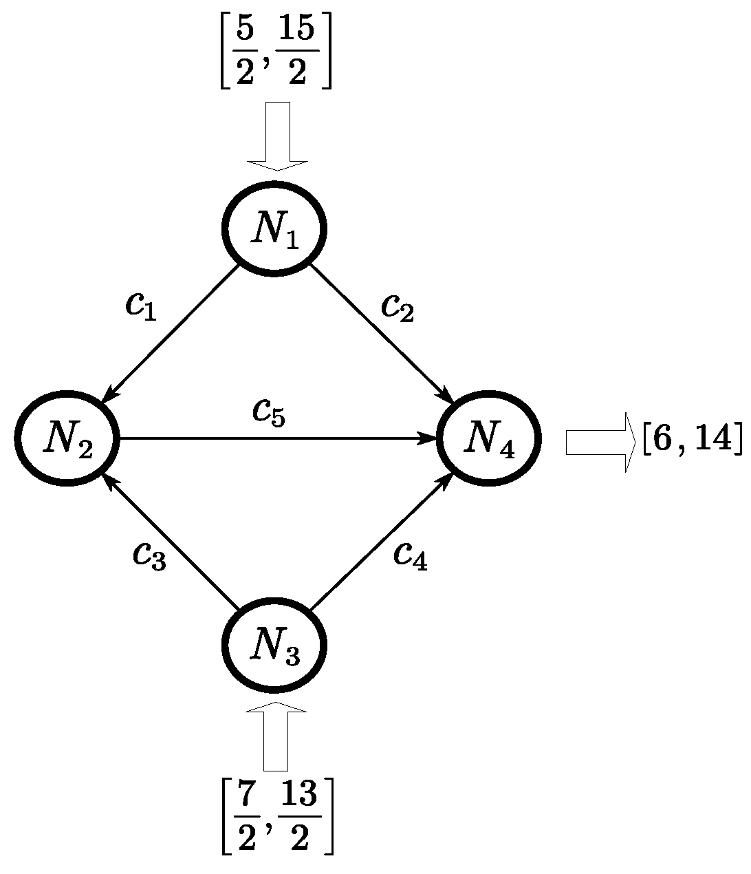
In this section, an example is provided to demonstrate the application of the obtained theoretical results. The example has the network topology depicted in Figure 1.

Table 1. OD pairs and paths.

p	${\mathbf{OD}}_{\mathit{p}}$		${\mathit{\omega }}_{\mathit{p}}$
1	${\mathcal{N}}_1\to {\mathcal{N}}_4$	$a_1$	$(c_1,c_5)$
		$a_2$	$\left(c_2\right)$
2	${\mathcal{N}}_3\to {\mathcal{N}}_4$	$a_3$	$(c_3,c_5)$
		$a_4$	$\left(c_4\right)$

summarizes the constituent paths of each OD pair.

The network consists of four nodes: $\mathcal{N}=\{{\mathcal{N}}_1,{\mathcal{N}}_2,{\mathcal{N}}_3,{\mathcal{N}}_4\}$ and five arcs: $\mathcal{C}=\{c_1,c_2,c_3,c_4,c_5\}$. We assume that $\mathcal{V}=\{{\overline{\varrho }}_{c_1}^1,{\overline{\varrho }}_{c_2}^1,{\overline{\varrho }}_{c_3}^1,{\overline{\varrho }}_{c_4}^1,{\overline{\varrho }}_{c_5}^1\}=\{5,4,3,6,4\}$, $\mathcal{P}=\{\{{\mathcal{N}}_1,{\mathcal{N}}_4\},\{{\mathcal{N}}_3,{\mathcal{N}}_4\}\}$, $m=1$, $e=2$, and $\mathcal{D}=\{d_1^1\left({\epsilon }_1^1\right),d_2^1\left({\epsilon }_2^1\right)\}$, where $d_1^1=5$, $d_2^1=5$, ${\epsilon }_1^1=\frac{5}{2}$, ${\epsilon }_2^1=\frac{3}{2}$, then $d_1^1\left({\epsilon }_1^1\right)\in [\frac{5}{2},\frac{15}{2}]$, $d_2^1\left({\epsilon }_2^1\right)\in [\frac{7}{2},\frac{13}{2}]$. Let $({\mu }_1^1,{\mu }_2^1,{\mu }_3^1,{\mu }_4^1)=(2,\frac{3}{2},\frac{1}{2},1)$ and $({\lambda }_1^1,{\lambda }_2^1,{\lambda }_3^1,{\lambda }_4^1)=(5,4,3,6)$. The costs on each arc are chosen as follows:

$$\begin{array}{cccccc}\hfill H_{c_1}^1\left({\varrho }_1^1\right)& =({\varrho }_1^1,{\varrho }_1^1),\hfill & \hfill H_{c_2}^1\left({\varrho }_2^1\right)& =(4{\varrho }_2^1,5{\varrho }_2^1),\hfill & \hfill H_{c_3}^1\left({\varrho }_3^1\right)& =(2{\varrho }_3^1,3{\varrho }_3^1),\hfill \\ \hfill H_{c_4}^1\left({\varrho }_4^1\right)& =(5{\varrho }_4^1,6{\varrho }_4^1),\hfill & \hfill H_{c_5}^1\left({\varrho }_1^1\right)& =({\varrho }_1^1,2{\varrho }_1^1),\hfill & \hfill H_{c_5}^1\left({\varrho }_3^1\right)& =({\varrho }_3^1,2{\varrho }_3^1).\hfill \end{array}$$

By a direct calculation, we derive the costs on four different paths:

$$\begin{array}{cc}\hfill H_1^1\left({\varrho }_1^1\right)=H_{a_1}^1\left({\varrho }_1^1\right)+H_{a_5}^1\left({\varrho }_1^1\right)=(2{\varrho }_1^1,3{\varrho }_1^1),& H_2^1\left({\varrho }_2^1\right)=H_{a_2}^1\left({\varrho }_2^1\right)=(4{\varrho }_2^1,5{\varrho }_2^1),\hfill \\ \hfill H_3^1\left({\varrho }_3^1\right)=H_{a_3}^1\left({\varrho }_3^1\right)+H_{a_5}^1\left({\varrho }_3^1\right)=(3{\varrho }_3^1,5{\varrho }_3^1),& H_4^1\left({\varrho }_4^1\right)=H_{a_4}^1\left({\varrho }_4^1\right)=(5{\varrho }_4^1,6{\varrho }_4^1).\hfill \end{array}$$

Setting $\varrho =({\varrho }_1^1,{\varrho }_2^1,{\varrho }_3^1,{\varrho }_4^1)=(3,2,1,4)$. Obviously, $\varrho \in Q$ is a feasible network flow. Thus,

$$H_1^1\left({\varrho }_1^1\right)=(6,9),H_2^1\left({\varrho }_2^1\right)=(8,10),H_3^1\left({\varrho }_3^1\right)=(3,5),H_4^1\left({\varrho }_4^1\right)=(20,24).$$

Now, we verify that the feasible flow $\varrho$ is a strict vector equilibrium flow. For OD pairs $\{{\mathcal{N}}_1,{\mathcal{N}}_4\}$, $\{{\mathcal{N}}_3,{\mathcal{N}}_4\}$, we choose $\overline{\Theta }=(0,1)$ and $\overline{\Xi }=(1,1)$; it holds that

$$\{\begin{array}{c}\mathrm{cone}(H_2^1\left({\varrho }_2^1\right)+{\mathbb{R}}_{+}^2-H_1^1\left({\varrho }_1^1\right))\cap (\mathrm{cone}(\overline{\Theta }-\overline{\Xi })\setminus \left\{0\right\})=\varnothing \hfill \\ H_2\left(\varrho \right)-H_1\left(\varrho \right)\ne 0\hfill \end{array}$$

and

$$\{\begin{array}{c}\mathrm{cone}(H_4^1\left({\varrho }_4^1\right)+{\mathbb{R}}_{+}^2-H_3^1\left({\varrho }_3^1\right))\cap (\mathrm{cone}(\overline{\Theta }-\overline{\Xi })\setminus \left\{0\right\})=\varnothing \hfill \\ H_4\left(\varrho \right)-H_3\left(\varrho \right)\ne 0\hfill \end{array}$$

Since the arc flow ${\varrho }_{c_5}^1$ is

$${\varrho }_{c_5}^1=\sum _{i\in \mathcal{I}}\sum _{k\in {\omega }_i}{\delta }_{ck}{\varrho }_k^j={\varrho }_1^1+{\varrho }_3^1=4={\overline{\varrho }}_{c_5}^1,$$

it follows from Definition 3 that arc $c_5$ is a saturated arc of flow $\varrho$, paths 3 and 5 are saturated paths of flow $\varrho$. Hence, by Definition 6, we obtain that $\varrho$ is a strict vector equilibrium flow.

Next, we show that $\varrho =({\varrho }_1^1,{\varrho }_2^1,{\varrho }_3^1,{\varrho }_4^1)=(3,2,1,4)$ is a solution of the following variational inequality:

$$\langle H\left(\varrho \right),{(\chi -\varrho )}^{\prime }\rangle \notin -{\mathbb{R}}_{+}^2\setminus \left\{0\right\},\forall \chi \in Q.$$

(10)

We take $\chi =({\chi }_1^1,{\chi }_2^1,{\chi }_3^1,{\chi }_4^1)=(3,3,1,4)$; it is obvious that $\chi \in Q$. Direct computation shows that

$$\begin{array}{ccc}& & \langle H\left(\varrho \right),{(\chi -\varrho )}^{\prime }\rangle \hfill \\ & & =\langle (H_1^1\left({\varrho }_1^1\right),H_2^1\left({\varrho }_2^1\right),H_3^1\left({\varrho }_3^1\right),H_4^1\left({\varrho }_4^1\right)),{({\chi }_1^1-{\varrho }_1^1,{\chi }_2^1-{\varrho }_2^1,{\chi }_3^1-{\varrho }_3^1,{\chi }_4^1-{\varrho }_4^1)}^{\prime }\rangle \hfill \\ & & =〈\left(\begin{array}{cccc}2{\varrho }_1^1& 4{\varrho }_2^1& 3{\varrho }_3^1& 5{\varrho }_4^1\\ 3{\varrho }_1^1& 5{\varrho }_2^1& 5{\varrho }_3^1& 6{\varrho }_4^1\end{array}\right),{\left(\begin{array}{cccc}3-{\varrho }_1^1,& 3-{\varrho }_2^1,& 1-{\varrho }_3^1,& 4-{\varrho }_4^1\end{array}\right)}^{\prime }〉\hfill \\ & & ={\left(\begin{array}{c}2{\varrho }_1^1(3-{\varrho }_1^1)+4{\varrho }_2^1(3-{\varrho }_2^1)+3{\varrho }_3^1(1-{\varrho }_3^1)+5{\varrho }_4^1(4-{\varrho }_4^1)\\ 3{\varrho }_1^1(3-{\varrho }_1^1)+5{\varrho }_2^1(3-{\varrho }_2^1)+5{\varrho }_3^1(1-{\varrho }_3^1)+6{\varrho }_4^1(4-{\varrho }_4^1)\end{array}\right)}^{\prime }\hfill \\ & & =\left(\begin{array}{c}8,10\end{array}\right)\notin -{\mathbb{R}}_{+}^2\setminus \left\{0\right\}.\hfill \end{array}$$

Therefore, the strict vector equilibrium flow $\varrho =(3,2,1,4)$ is a solution of variational inequality (10).

6. Conclusions

This paper considered the strict network equilibrium flows for a multi-product supply–demand network with capacity constraints and uncertain demands, where the uncertain demands were assumed to be in a closed interval. The main contribution is theoretical in nature, in that we derived the existence results of strict network equilibrium flows by virtue of the Fan–Browder fixed point theorem based on a single criterion cost function and showed that such a strict network equilibrium flow for a multi-product supply–demand network with capacity constraints and uncertain demands is equivalent to a vector variational inequality when considering both real value and vector value cost function, and we developed a scalarization method for strict vector equilibrium flows based on vector-valued cost functions by using Gerstewitz’s function. The results obtained in this paper provide a viable approach to solving the multi-product, multi-criteria supply–demand network equilibrium model with capacity constraints and uncertain demands.

In this paper, we presented an analytical framework based on the concept of network equilibrium to attain optimal performance for a multi-product supply–demand network with capacity constraints and uncertain demands. In future research, designing concrete simulation experiments and developing substantial areas of applications of the theory presented in our paper should be considered as a potential research project.

References

1. Wardrop, J.G. Some theoretical aspects of road traffic research. Proc. Inst. Civ. Eng. 1952, 1, 325–378. [Google Scholar] [CrossRef]
2. Dong, J.; Zhang, D.; Nagurney, A. A supply chain network equilibrium model with random demands. Eur. J. Oper. Res. 2004, 156, 194–212. [Google Scholar] [CrossRef]
3. Meng, Q.; Huang, Y.K.; Chen, R.L. A note on supply chain network equilibrium models. Transport. Res. E 2008, 184, 13–23. [Google Scholar] [CrossRef]
4. Nagurney, A. On the relationship between supply chain and transportation network equilibria: A supernetwork equivalence with computations. Transport. Res. E 2006, 42, 293–316. [Google Scholar] [CrossRef]
5. Nagurney, A.; Dong, J.; Zhang, D. A supply chain network equilibrium model. Transport. Res. E 2002, 38, 281–303. [Google Scholar] [CrossRef]
6. Chen, G.Y.; Yen, N.D. On the Variational Inequality Model for Network Equilibrium; Internal Report 196; Department of Mathematics, University of Pisa: Pisa, Italy, 1993; pp. 724–735. [Google Scholar]
7. Cheng, T.C.E.; Wu, Y.N. A multi-product, multi-criterion supply-demand network equilibrium model. Oper. Res. 2006, 54, 544–554. [Google Scholar] [CrossRef]
8. Khanh, P.O.; Luu, L.M. On the existence of solutions to vector quasivariational inequalities and quasicomplementarity problems with applications to traffic network equilibria. J. Optimiz. Theory Appl. 2004, 123, 533–548. [Google Scholar] [CrossRef]
9. Khanh, P.O.; Luu, L.M. Some existence results for quasi-variational inequalities involving multifunctions and applications to traffic equilibrium problems. J. Global Optim. 2005, 32, 551–568. [Google Scholar] [CrossRef]
10. Lin, Z. The study of traffic equilibrium problems with capacity constraints of arcs. Nonlinear Anal. Real World Appl. 2010, 11, 2280–2284. [Google Scholar] [CrossRef]
11. Lin, Z. On existence of vector equilibrium flows with capacity constraints of arcs. Nonlinear Anal. Theory Methods Appl. 2010, 72, 2076–2079. [Google Scholar] [CrossRef]
12. Li, S.J.; Teo, K.L.; Yang, X.Q. Vector equilibrium problems with elastic demands and capacity constraints. J. Global Optim. 2007, 37, 647–660. [Google Scholar] [CrossRef]
13. Li, S.J.; Teo, K.L.; Yang, X.Q. A remark on a standard and linear vector network equilibriium problem with capacity constraints. Eur. J. Oper. Res. 2008, 184, 13–23. [Google Scholar] [CrossRef]
14. Li, S.J.; Yang, X.Q.; Chen, G.Y. A note on vector network equilibrium principles. Math. Methods Oper. Res. 2008, 184, 13–23. [Google Scholar] [CrossRef]
15. Cao, J.D.; Li, R.X.; Huang, W.; Guo, J.H.; Wei, Y. Traffic network equilibrium problems with demands uncertainty and capacity constraints of arcs by scalarization approaches. Sci. China Technol. Sci. 2018, 61, 1642–1653. [Google Scholar] [CrossRef]
16. Wei, H.Z.; Chen, C.R.; Wu, B.W. Vector network equilibrium problems with uncertain demands and capacity constraints of arcs. Optim. Lett. 2021, 15, 1113–1131. [Google Scholar] [CrossRef]
17. Wu, Y.N.; Cheng, T.C.E. Benson efficiency of a multi-criterion network equilibrium model. Pac. J. Optim. 2009, 5, 443–458. [Google Scholar]
18. Wu, Y.N.; Peng, Y.C.; Peng, L.; Xu, L. Super efficiency of multicriterion network equilibrium model and vector variational inequality. J. Optim. Theory App. 2012, 153, 485–496. [Google Scholar] [CrossRef]
19. Gong, X.H. Efficiency and Hening efficiency for vector equilibrium problems. J. Optimiz. Theory App. 2001, 108, 139–154. [Google Scholar] [CrossRef]
20. Cheng, Y.H.; Fu, W.T. Strong efficiency in a locally convex space. Math. Methods Oper. Res. 1999, 50, 373–384. [Google Scholar] [CrossRef]
21. Yu, G.L.; Zhang, Y.; Liu, S.Y. Strong duality with strict efficiency in vector optimization involving nonconvex set-valued maps. J. Math. 2017, 37, 223–230. [Google Scholar]
22. Konnov, I.V. Vector network equilibrium problems with elastic demands. J. Global Optim. 2013, 57, 521–531. [Google Scholar] [CrossRef]
23. Browder, F.E. The fixed point theory of multi-valued mappings in topological vector spaces. Math. Ann. 1968, 177, 283–301. [Google Scholar] [CrossRef]
24. Fan, K. A generalization of Tychonoffs fixed point theorem. Math. Ann. 1961, 142, 305–310. [Google Scholar] [CrossRef]
25. Chen, G.Y.; Goh, C.J.; Yang, X.Q. Vector network equilibrium problems and nonlinear scalarization methods. Math. Methods Oper. Res. 1999, 49, 239–253. [Google Scholar]
26. Chen, G.Y.; Yang, X.Q. Characterizations of variable domination structures via nonlinear scalarization. J. Optim. Theory App. 2002, 112, 97–110. [Google Scholar] [CrossRef]
Figure 1. Network topology of the example.
Axioms 13 00263 g001