Packing Spheres into a Minimum-Height Parabolic Container

Abstract

Sphere packing consists of placing several spheres in a container without mutual overlapping. While packing into regular-shape containers is well explored, less attention is focused on containers with nonlinear boundaries, such as ellipsoids or paraboloids. Packing n-dimensional spheres into a minimum-height container bounded by a parabolic surface is formulated. The minimum allowable distances between spheres as well as between spheres and the container boundary are considered. A normalized Φ-function is used for analytical description of the containment constraints. A nonlinear programming model for the packing problem is provided. A solution algorithm based on the feasible directions approach and a decomposition technique is proposed. The computational results for problem instances with various space dimensions, different numbers of spheres and their radii, the minimal allowable distances and the parameters of the parabolic container are presented to demonstrate the efficiency of the proposed approach.

1. Introduction

Sphere packing is a well-studied area of research that involves arranging identical or non-identical spherical items within a given volume (container), subject to certain constraints. This problem has a wide range of applications, making it a versatile and important topic in both theoretical and practical contexts [1]. According to the typology of packing and cutting problems introduced in [2], packing problems are considered in two main formulations: open dimension problems (ODP) and knapsack problems. The ODP is aimed at optimizing the dimension(s) of a container, while packing the maximum number of identical objects or maximizing the total volume of packed objects is a knapsack problem. Typically, continuous nonlinear programming (NLP) models are used to formulate an ODP, while for the knapsack problem, mixed integer NLP models are implemented.

Our interest in irregular containers is motivated by the following considerations. Packing problems for regular-shaped containers (rectangles, circles) are well studied for 2D objects, such as circles [3], ovals [4,5] and ellipses [6,7,8]. Rich theoretical and empirical results are presented in these papers, where various NLP models and exact/heuristic/metaheuristic solution techniques are accompanied by extensive computational experiments to demonstrate the efficiency of the proposed approaches. Different NLP models and solution algorithms for packing 3D objects into regular 3D containers (cuboids, spheres, and cylinders) can be found, e.g., in [9,10] for spherical and in [11] for ellipsoidal shapes, together with corresponding empirical results obtained for different numbers of objects and various container shapes. In all these works, geometric tools for modeling non-overlapping and containment conditions in Euclidean and non-Euclidean [4,5,9] metrics are provided. Algorithms based on combinations of smart heuristics and nonlinear optimization techniques are designed. The proposed solution approaches allow us to find the optimal solutions for small and medium-sized instances, while reasonably good feasible solutions are obtained for larger instances. However, as was highlighted in review papers [12,13,14,15], challenging packing problems in irregular containers are much less investigated. Several publications consider ellipsoidal containers [16,17], while there are only a few works focusing on packing for multiply connected domains and cardioids [18] and paraboloids [19]. Sphere packing into irregular containers arises in, e.g., material science [20,21] and nanotechnology [22]. A simple application of sphere packing into a parabolic container can be found in the food industry [23], where a parabolic dish container must be designed to store candies. To the best of our knowledge, in the n-dimensional case, the problem of packing spheres into an optimized parabolic container has not been considered before.

A brief review of the papers related to packing in irregular containers is provided below. An approach to constructing analytical non-intersection and containment conditions for non-oriented convex two-dimensional objects, defined by second-order curves, is proposed in [16]. This approach was applied to a problem of packing circles into an ellipse and minimizing the ellipse size. Packing algorithms applied to different-shaped two-dimensional domains are studied in [18], including rectangles, ellipses, crosses, multiply connected domains and even cardioid shapes. The authors introduce a novel approach centered around the concept of “image” disks, enabling the study of packing within fixed containers. Paper [19] focuses on Apollonian circle packing. The method has been used in various models, including geological sheer bands. Mathematical equations utilizing hyperbolas and ellipses are applied. This approach is applicable to a generic, closed, convex contour given the parametrization of its boundary. In the aerospace industry, packing into parabolic or other non-traditional containers is a significant challenge due to the specific shapes and delicate nature of many components [19]. The container is divided by horizontal racks into sub-containers. The proposed mathematical model considers the minimal and maximal allowable distances between objects subject to the behavior constraints of the mechanical system (equilibrium, moments of inertia and stability constraints). The paper describes a solution approach based on the multistart strategy, Shor’s r-algorithm and accelerated search for the terminal nodes of the solution tree.

The objective of this paper is to develop a modeling and solutions approach to an ODP that consists of packing n-dimensional spheres into a minimum-height parabolic container. For analytical description of the placement constraints, the Φ-function technique [24] is used. This approach allows us to present mathematical models of optimized packing problems in the form of continuous NLP problems. To describe the containment of spheres in the parabolic container, a new Φ-function for the nD case is introduced. Using a section of the nD paraboloid and spheres by hyperplanes, it is iteratively reduced to consideration of the Φ-function in the 2D case. The Φ-function involves an additional variable parameter that is dynamically adjusted by solving a one-dimensional optimization problem. An approach based on the feasible directions method (FDM) [25] is developed considering the special properties of the Φ-function.

The contributions of the paper are as follows:

• A new problem of packing spheres into a minimum-height parabolic container in n-dimensional space;
• A new Φ-function for analytical description of the containment of a sphere into a parabolic container in n-dimensional space;
• An approach based on the feasible directions scheme considering the specific characteristics of the Φ-function.
• New benchmarks for various sphere radii and the parameters of the parabolic container in n-dimensional space for n = 2, 3, 4, 5.

The remainder of this paper is organized as follows. Section 2 describes the problem statement. Section 3 introduces geometrical tools for constructing a mathematical model of the packing problem. A mathematical model is formulated in Section 4. Section 5 presents a modification of the FDM. Section 6 provides the computational results for problem instances in several dimensions, with different numbers of spheres and their radii and various values of the minimal allowable distances and the parameters of the parabolic container. Section 7 concludes.

2. Problem Statement

Let a convex domain bounded by a parabolic surface and a hyperplane be defined in n-dimensional Euclidean space ${ℝ}^n$ as follows: $P_n(h)=P_n\cap H_n$ where $P_n=\{X=(x_1,x_2,\dots ,x_n)\in {ℝ}^n:{\displaystyle \sum _{i=1}^{n-1}}{x}_i^2-2p{x}_n\le 0\}$ and $H_n=\{X\in {ℝ}^n:x_n-h\le 0\}$, i.e.,

$$P_n(h)=\{X\in {ℝ}^n:\stackrel{n-1}{{\displaystyle \sum }_{i=1}}{x}_i^2-2p{x}_n\le 0, x_n-h\le 0\}.$$

(1)

Further, we refer the domain $P_n(h)$ to a container of variable height $h>0$, with the predefined parameter $p>0$.

And let a collection of nD spheres $S_j$,$j\in J=\{1,2,\dots ,m\}$ with variable centers $y_j=(y_{j1},y_{j2},\dots ,y_{jn})\in {ℝ}^n$,$j\in J$, be given and denoted by

$$S_j(y_j)=\{X\in {ℝ}^n:\hspace{0.17em}\Vert X-y_j\Vert -r_j\le 0\},j\in J.$$

(2)

In addition, the minimal allowable distances between each pair of spheres $S_t(y_t)$ and $S_j(y_j)$, as well as between a sphere $S_j(y_j)$ and the boundary of the container $P_n(h)$, are given, respectively, as ${\delta }_{tj}$ and ${\delta }_j$.

Packing problem. Pack spheres $S_j(y_j)$, $j\in J$, into the minimum-height container $P_n(h)$, considering the minimal allowable distances ${\delta }_{tj}$, $t<j\in J$, and ${\delta }_j$, $j\in J$.

To describe the placement constraints of the packing problem analytically, the Φ-function technique is used. For the reader’s convenience, the main definitions of the phi-function are provided in Appendix A. More details can be found in, e.g., Chapter 15 of [26].

The distance constraint for two spheres can be defined using the adjusted Φ-function in the form

$${\Phi }_{tj}(y_t,y_j)={\Vert y_t-y_j\Vert }^2-{(r_t+r_j+{\delta }_{tj})}^2.$$

Therefore,

$${\Phi }_{tj}(y_t,y_j)\ge 0\iff dist(S_t(y_t),S_j(y_j))\ge {\delta }_{tj},$$

$$dist(S_t(y_t),S_j(y_j))=\underset{a\in S_t(y_t),b\in S_j(y_j)}{\min }\Vert a-b\Vert , a=(a_1,a_2,\dots ,a_n),b=(b_1,b_2,\dots ,b_n).$$

In Section 3, we introduce a continuous and everywhere defined function that allows us to describe the containment of each sphere into a parabolic container.

3. The Φ-Function for Containment Constraints

To describe analytically the containment constraint, $S_j(y_j)\subset P_n(h)\iff \mathrm{int}{S}_j(y_j)\cap P_n^{*}(h)=\varnothing$, let us define a phi-function for an nD sphere $S_j(y_j)$ (2) and the object $P_n^{*}(h)={ℝ}^n\backslash \mathrm{int}{P}_n(h)$ (the compliment of the container $P_n(h)$ interior to the whole space ${ℝ}^n$).

Note that $P_n^{*}(h)=P_n^{*}\cup H_n^{*}$, where $H_n=\{X\in {ℝ}^n:x_n-h\ge 0\}$ and

$$P_n^{*}=\{X\in {ℝ}^n:\stackrel{n-1}{{\displaystyle \sum }_{i=1}}{x}_i^2-2p{x}_n\ge 0\}.$$

(3)

A $\Phi$-function for a sphere $S_j(y_j)$ and the object $P_n^{*}(h)$ can be stated in the following form:

$${\Phi }_j^{*}(y_j,y_{jn},h)=\min \{ {\Phi }_j(y_j)-{\delta }_j,{\Theta }_j(y_{jn},h)\},$$

(4)

where ${\Phi }_j(y_j)$ is a Φ-function for a sphere $S_j(y_j)$ and the object $P_n^{*}$, and ${\Theta }_j(y_{jn},h)=h-y_{jn}-r_j$ is a $\Phi$-function for a sphere $S_j(y_j)$ and a half-space $H_n^{*}$.

Let us define a Φ-function for a sphere $S_j(y_j)$ and the object $P_n^{*}$. We state that $S_j(y_j)\subset P_n$ if $P_n^{*}\cap \mathrm{int}{S}_j(y_j)=\varnothing$.

Firstly, construct an (n − 1)D hyperplane $K_1$ passing through axis $O{x}_n$ of $P_n$ and the center $y_j=(y_{j1},y_{j2},\dots ,y_{jn})$ of the nD sphere $S_j(y_j)$. Then, the section $K_1\cap P_n$ yields the parabolic domain

$$P_{n-1}=\{X\in {ℝ}^{n-1}:\hspace{0.17em}-z_1^2-\stackrel{n-1}{{\displaystyle \sum }_{i=3}}{x}_i^2+2p{x}_n=0\},$$

where $z_1=\pm \sqrt{x_1^2+x_2^2},$ while the section $K_1\cap S_j(y_j)$ yields the (n − 1)D-sphere $S_{j(n-1)}$ of radius $r_j$ and the center $y_{j(n-1)}=(z_{j1},y_{j3},\dots ,y_{jn}),$$z_{j1}=\mathrm{sign}(y_{j1})\sqrt{y_{j1}^2+y_{j2}^2}$.

By analogy, an (n − 2)D-hyperplane $K_2$ passing through axis $O{x}_n$ of $P_{n-1}$ and the center $y_{j(n-1)}$ of $S_{j(n-1)}$ is constructed. Then, the section $K_2\cap P_{n-1}$ yields the parabolic domain

$$P_{n-2}=\{X\in {ℝ}^{n-2}:-\hspace{0.17em}{z}_2^2-\stackrel{n-1}{{\displaystyle \sum }_{i=4}}{x}_i^2+2p{x}_n=0\},$$

where $z_2=\pm \sqrt{{\displaystyle {\sum }_{i=1}^3{x}_i^2}}$, while the section $K_2\cap S_{j(n-1)}$ yields the (n − 2)D-sphere $S_{j(n-2)}$ of radius $r_j$ and the center $y_{j(n-2)}=(z_{j2},y_{j4},\dots ,y_{jn}),$ $z_{j2}=\mathrm{sign}(z_{j1})\sqrt{{\displaystyle {\sum }_{i=1}^3{y}_{ji}^2}}$.

The iterative procedure continues until the 2D parabolic domain $P_2=\{X\in {ℝ}^2:\hspace{0.17em}-z_{(n-1)}^2+2p{x}_n=0\}$ with $z_{n-1}=\mathrm{sign}(z_{j(n-2)})\sqrt{{\displaystyle {\sum }_{i=1}^{n-1}{x}_i^2}}$ and the 2D sphere $S_{j2}$ of radius $r_j$ and the center $(z_{j(n-1)},y_{jn})$ are obtained.

Note that $\mathrm{sign}(z_{j(n-2)})=\mathrm{sign}(z_{j(n-3)})=\dots =\mathrm{sign}(z_{j1})=\mathrm{sign}(y_{j1})$. This means that the construction of the Φ-function for the object $P_n^{*}$ (3) and the nD sphere $S_j(y_j)$ (2) is reduced to deriving the Φ-function for the object $P_2^{*}$ and the 2D sphere $S_{j2}$.

Let an equation of the tangent ${\mathsf{\Upsilon }}_j$ to the boundary of $P_2$ be given

$$f(z_{n-1},x_n,t_j)=-z_{n-1}\sqrt{2p}{t}_j+p(x_n+t_j^2)=0$$

for any $t_j\in {ℝ}^1$. Note that different tangents ${\mathsf{\Upsilon }}_j(t_j)$ can be generated for different values of $t_j$.

Let a point $(z_{n-1},x_n)=(t_j\sqrt{2p},t_j^2)$ be a tangency point of ${\mathsf{\Upsilon }}_j(t_j)$ and the boundary of $P_2$. Then, the normal equation of ${\mathsf{\Upsilon }}_j(t_j)$ takes the form

$$f_j(z_{n-1},x_n,t_j)=-\frac{z_{n-1}\sqrt{2p}{t}_j-p(x_n+t_j^2)}{\sqrt{2p{t}_j^2+p^2}}=0.$$

(5)

Thus, the normalized Φ-function for the 2D sphere $S_{j2}$ and the half-plane specified by the inequality $f_j(z_{n-1},x_n,t_j)\le 0$ can be defined as follows:

$${\Phi }_{j0}(z_{j(n-1)},y_{jn},t_j)=f_j(z_{j(n-1)},y_{jn},t_j)-r_j.$$

(6)

Substituting $f_j(z_{n-1},x_n,t_j)$ (5) into (6), the function ${\omega }_j(t_j)=(-z_{j,(n-1)}\sqrt{2p}{t}_j-p(y_{jn}+t_j^2))/\sqrt{2p{t}_j^2+p^2}$ can be defined.

Then, we search for $t_j^{*}$ at which the function ${\omega }_j(t_j^{*})$ reaches the minimum corresponding to the distance between the center of $S_{j2}$ and the boundary of $P_2$. Consequently, bearing in mind $z_{n-1}=\pm \sqrt{{\displaystyle {\sum }_{i=1}^{n-1}{x}_i^2}}$, the normalized Φ-function for $S_j(y_j)$ and $P_2^{*}$ (3) takes the form

$${\Phi }_j(y_j)=\underset{t_j\in [{\beta }_{j1},{\beta }_{j2}]}{\min }{\Phi }_{j0}(z_{j(n-1)},y_{jn},t_j).$$

(7)

To find the optimal value of $t_j\in [{\beta }_{j1},{\beta }_{j2}]$, a bisection technique [25] is applied.

Let us consider two cases for the locations of the center of $S_{j2}$ with respect to $P_2$: case 1 corresponds to $(z_{j(n-1)},y_{jn})\in P_2$; case 2 corresponds to $(z_{j(n-1)},y_{jn})\notin P_2.$

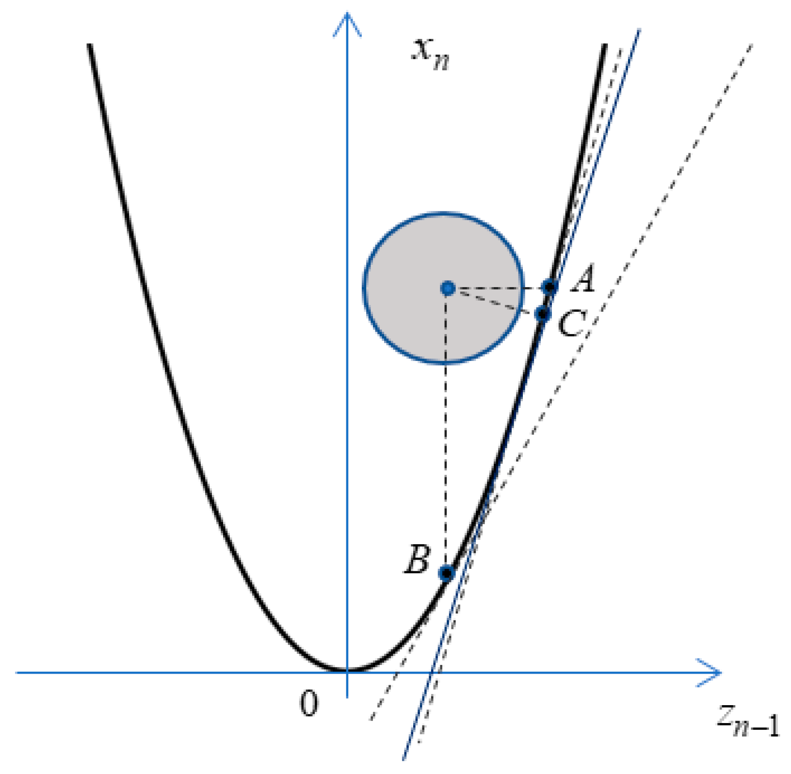
Assume $({\stackrel{⌢}{z}}_{j(n-1)},{\stackrel{⌢}{y}}_{jn})\in P_2$ and ${\stackrel{⌢}{y}}_{jn}\ge 0$. Here, $({\stackrel{⌢}{z}}_{j(n-1)},{\stackrel{⌢}{y}}_{jn})$ is the center point of the sphere $S_{j2}$. Let us consider two tangents ${\mathsf{\Upsilon }}_j(t_{j1})$ and ${\mathsf{\Upsilon }}_j(t_{j2})$ to $\mathrm{fr}{P}_2$ at points $A(\sqrt{2p{\stackrel{⌢}{y}}_{jn}},{\stackrel{⌢}{y}}_{jn})$ and $B({\stackrel{⌢}{z}}_{j(n-1)},{\stackrel{⌢}{z}}_{j(n-1)}^2/(2p))$ for corresponding $t_{j1}=\sqrt{{\stackrel{⌢}{y}}_{jn}}$ and $t_{j2}={\stackrel{⌢}{z}}_{j(n-1)}/\sqrt{2p}$ (Figure 1). Therefore, $[{\beta }_{j1},{\beta }_{j2}]=[{\stackrel{⌢}{z}}_{j(n-1)}/\sqrt{2p},\sqrt{{\stackrel{⌢}{y}}_{jn}}]$.

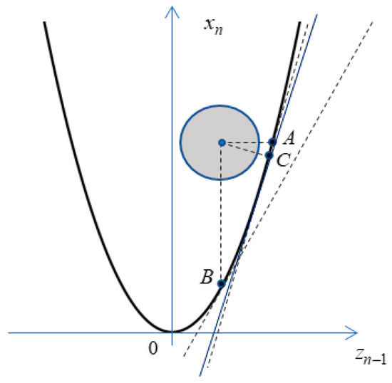
Figure 1. Illustration of interaction of $S_{j2}$ and the boundary of $P_2$ in 2D.

In Figure 1, the segment $AB$ of the parabola that corresponds to $t_j\in [{\beta }_{j1},{\beta }_{j2}]$ is shown. The tangent ${\mathsf{\Upsilon }}_j(t_j^{*})$ at the point $C$$(\sqrt{2p{\stackrel{⌢}{y}}_{jn}},{\stackrel{⌢}{y}}_{jn},t_j^{*})$ corresponds to $t_j^{*}=\underset{t_j\in [{\beta }_{j1},{\beta }_{j2}]}{\arg \min }{\Phi }_{j0}({\stackrel{⌢}{z}}_{j(n-1)},{\stackrel{⌢}{y}}_{jn},t_j)$.

Let $(z_{j(n-1)},y_{jn})\in P_2$ (case 1); then,

$$\begin{array}{l}[{\beta }_{j1},{\beta }_{j2}]=\{\begin{array}{l}[\frac{z_{j(n-1)}}{\sqrt{2p}},\sqrt{y_{jn}}] \mathrm{if} z_{j(n-1)}\ge 0\hspace{0.17em}\hspace{0.17em}(\mathrm{case}\hspace{0.17em}1.1)\\ [-\sqrt{y_{jn}},\frac{z_{j(n-1)}}{\sqrt{2p}}] \mathrm{if} z_{j(n-1)}<0\hspace{0.17em}\hspace{0.17em}(\mathrm{case}\hspace{0.17em}1.2)\end{array}\\ \end{array}.$$

(8)

Let $(z_{j(n-1)},y_{jn})\notin P_2$(case 2); then,

$$[{\beta }_{j1},{\beta }_{j2}]=\{\begin{array}{l}[\sqrt{y_{jn}},\frac{z_{j(n-1)}}{\sqrt{2p}}] \mathrm{if} z_{j(n-1)}\ge 0, y_{jn}\ge 0\hspace{0.17em}(\mathrm{case}\hspace{0.17em}2.1)\\ [-\frac{\left|z_{j(n-1)}\right|}{\sqrt{2p}},\frac{\left|z_{j(n-1)}\right|}{\sqrt{2p}}] \mathrm{if} y_{jn}<0\hspace{0.17em}(\mathrm{case}\hspace{0.17em}2.2)\\ [-\frac{z_{j(n-1)}}{\sqrt{2p}},\sqrt{y_{jn}}] \mathrm{if} z_{j(n-1)}<0, y_{jn}\ge 0\hspace{0.17em}(\mathrm{case}\hspace{0.17em}2.3)\end{array}.$$

(9)

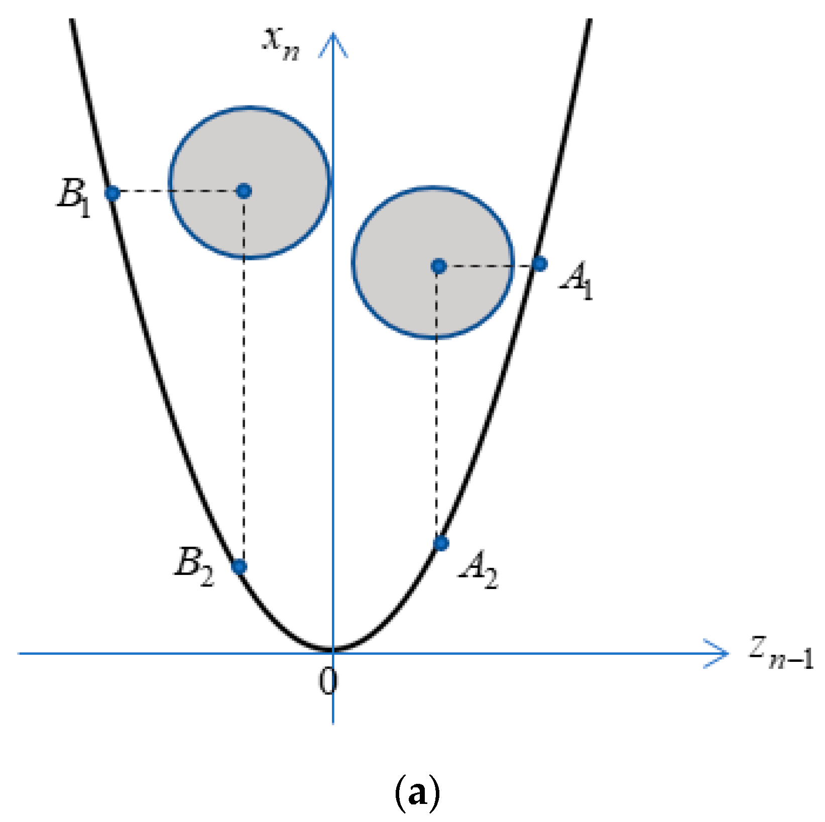
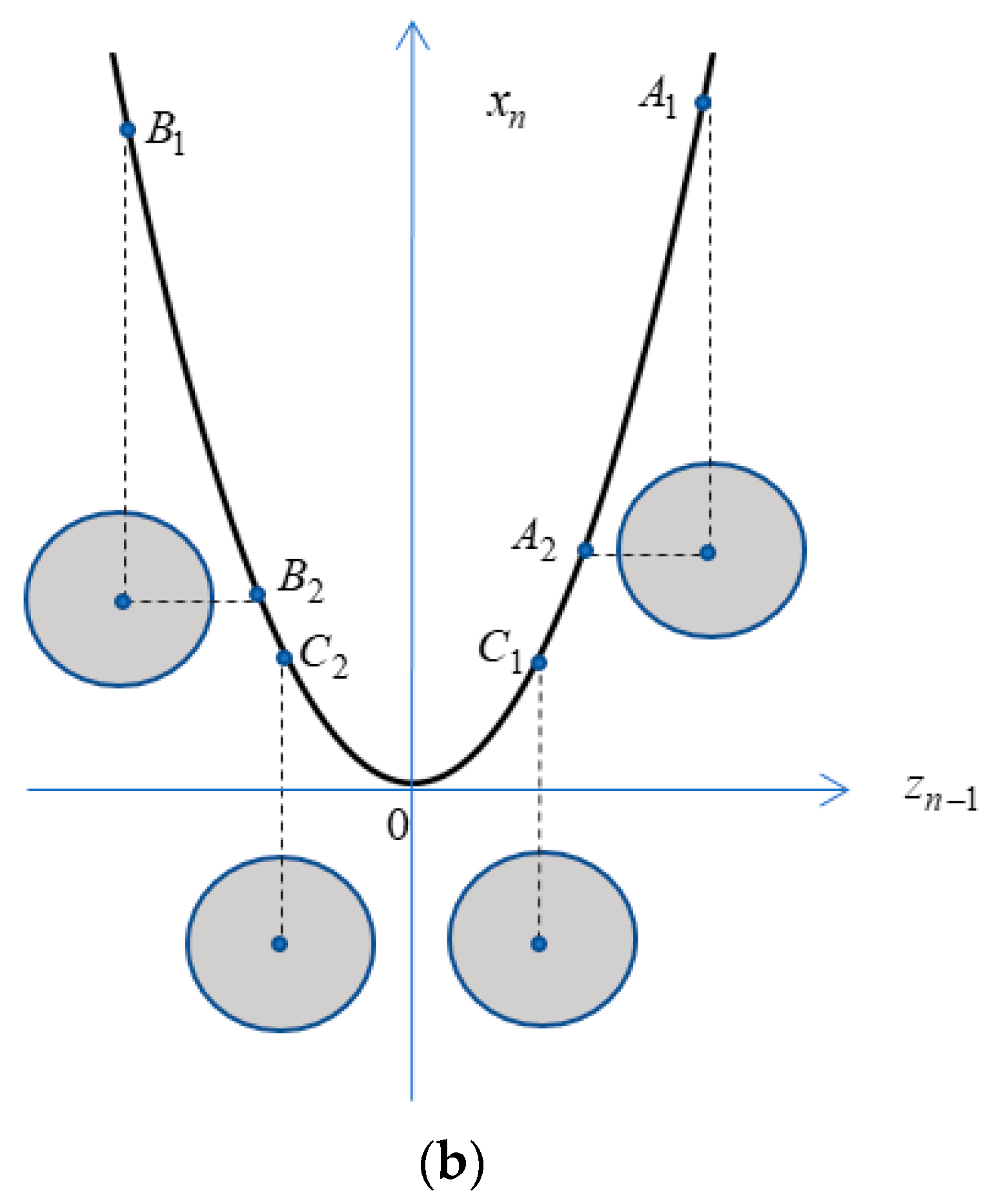
Figure 2 illustrates two cases: a sphere is arranged inside the parabolic domain $P_2$ ${\Phi }_j(y_j)\ge 0$(Figure 2a), and a sphere is arranged outside the parabolic domain $P_2$, ${\Phi }_j(y_j)<0$ (Figure 2b).

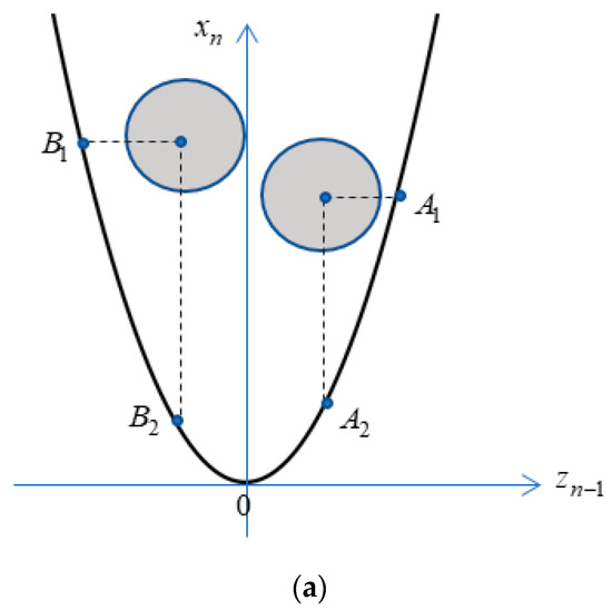
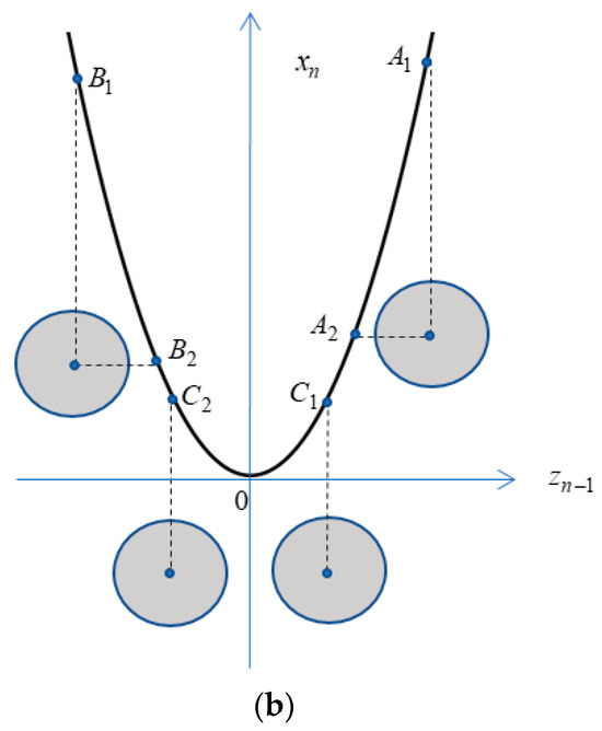
Figure 2. Arrangements of $S_{j2}$ with respect to $P_2$ for different $t_j\in [{\beta }_{j1},{\beta }_{j2}]$: (a) $(z_{j(n-1)},y_{jn})\in P_2$; (b) $(z_{j(n-1)},y_{jn})\notin P_2$.

In particular, to calculate $t\in [{\beta }_{j1},{\beta }_{j2}]$, $\mathrm{case}\hspace{0.17em}1.1$ (8) is used for the parabolic segment $A_1,A_2$, while $\mathrm{case}\hspace{0.17em}1.2$ (8) is used for the parabolic segment $B_1,B_2$ (Figure 2a); $\mathrm{case}\hspace{0.17em}2.1$ (9) is used for the parabolic segment $A_1,A_2$, $\mathrm{case}\hspace{0.17em}2.2$ (9) is used for the parabolic segment $C_1,C_2$, and $\mathrm{case}\hspace{0.17em}2.3$ in (9) is used for the parabolic segment $B_1,B_2$ (Figure 2b).

4. Mathematical Model

A mathematical model of the packing problem can be formulated as follows:

$$\underset{Y,h}{\min }h\hspace{0.17em}$$

(10)

subject to

$$\begin{gathered} {\Phi }_{tj}(y_t,y_j)={\Vert y_t-y_j\Vert }^2-{(r_t+r_j+{\delta }_{tj})}^2\ge 0, t<j\in J \\ {\Phi }_j^{*}(y_j,y_{jn},h)=\min \{ {\Phi }_j(y_j)-{\delta }_j,{\Theta }_j(y_{jn},h)\}\ge 0, j\in J \end{gathered}$$

(11)

where $Y=(y_1,y_2,\dots ,y_m)\in {ℝ}^{mn}$.

Note that the inequality ${\Phi }_j^{*}(y_j,y_{jn},h)\ge 0$ in (11) is equivalent to the system of inequalities ${\Phi }_j(y_j)-{\delta }_j\ge 0$ and ${\Theta }_j(y_{jn},h)\ge 0$ and ensures the arrangement of the nD sphere $S_j(y_j)$ fully inside the parabolic container $P_n(h)$$.$

The number of inequalities specifying the feasible region (11) is equal to $\chi =0.5m(m-1)+2m$. The dimensions of a solution matrix for $W$ are $(mn+1)\times \chi$.

Thus, the number of inequalities/variables in the inequality system (11) is increased drastically by enlarging $m$. The solution matrix is strongly sparse. The problem is NP-hard [27].

Since we cannot define $t_j$ explicitly, then we need to solve the optimization problems of the form (7) for each sphere $S_j(y_j)$ on each iteration of the solution process of the problem (10), (11). We do not use the solvers BARON [28] or IPOPT [29] for the original problem because of the dynamic nature of the Φ-function. Instead, a modification of the feasible directions method is developed.

The following solution strategy scheme for the problem (10), (11) is proposed:

• Take a sufficiently large height $h^0$ of the container that guarantees a placement of spheres $S_j(y_j)$, $j\in J,$ fully inside $P(h^0)$;
• Generate the sphere centers $y_j^0,$$j\in J,$ randomly so that $S_j(y_j^0)\subset P(h^0)$, $j\in J,$${\Phi }_{tj}(y_t^0,y_j^0)\ge 0, t<j\in J$;
• Apply the modification of the FDM to solve the problem (10), (11) for a set of feasible starting points.
• Select the best solution.

5. Solution Algorithm

In contrast to the problem considered in [30], in this study, the spheres are of different radii, and the Φ-function describing the containment of a sphere into the container involves an additional parameter, which is dynamically changed during the optimization process.

The FDM for the problem (10), (11) is implemented using the iterative formula

$$Y^{k+1}=Y^k+{\lambda }^k{Z}^k , k=0,1,2,\dots ,$$

(12)

where $Y^0\in W$(for $k=0$) is a starting feasible point, $Z^k$ is a search direction vector, and ${\lambda }^k>0$ is a parameter that controls the step size.

Let $\phi (Y)=h$ denote the objective function. A vector $Z^k$ in (12) should provide $Y^k\in W$. To search for a vector $Z^k$, the following linear programming problem is solved:

$$(Z^k,{\alpha }^k)=\arg \max \alpha \hspace{0.17em}\mathrm{s}.\mathrm{t}. \mathsf{\Upsilon }=(Z,\alpha )\in G^k,$$

(13)

$$\begin{array}{l}{G}^k=\{(Z,\alpha )\in {ℝ}^{\chi +1}:\hspace{0.17em}\nabla {\Phi }_{tj}(y_t^k,y_j^k)\cdot Z\ge \alpha , t<j\in J, \nabla {\Phi }_j(y_j^k)\cdot Z\ge \alpha , \\ \nabla {\Theta }_j(y_{jn}^k,h^k)\cdot Z\ge \alpha ,-\nabla \phi (h^k)\cdot Z\ge \alpha , \left|z_i\right|\le 1, i\in \Xi =\{1,2,\dots ,\chi \}\},\end{array}$$

(14)

where $Z=(z_1,z_2,\dots ,z_{\chi })\in {ℝ}^{\chi }$, $\alpha \in {ℝ}^1$, ${\Phi }_j(y_j^k)$ is constructed according to (7).

Note that in (11), each ${\Phi }_{tj}(y_t,y_j)$ is an inverse convex function, and each ${\Theta }_j(y_{jn},h)$ is a linear function. The vector of feasible directions may be orthogonal to the gradients of these constraints, so the inequalities $\nabla {\Phi }_{tj}(y_t^k,y_j^k)\cdot Z\ge \alpha$ and $\nabla {\Theta }_j(y_{jn}^k,h^k)\cdot Z\ge \alpha$ in (14) are replaced with $\nabla {\Phi }_{tj}(y_t^k,y_j^k)\cdot Z\ge 0$ and $\nabla {\Theta }_j(y_{jn}^k,h^k)\cdot Z\ge 0$, respectively.

To reduce the dimension of the problem (10), (11) and consequently of the problem (13), (14), a decomposition strategy [31] based on the degree of feasibility is employed.

When considering all the placed spheres, the majority of them are positioned at a significant distance from each other. The inequalities in the system (11) are satisfied with a considerable margin, and they can be disregarded when forming the optimization vector. At each step, only a subset of inequalities from the system (11) is considered, specifically those with a low degree of feasibility. During the optimization process, a parameter ${\epsilon }^k>0$ determining the degree of feasibility is adjusted dynamically, regulating the system constraints at each step. If an inequality is not considered in the optimization process at a certain step but is violated during the step’s execution, the admissibility is controlled using the parameter ${\lambda }^k$ in iterative Formula (12).

Let us denote the inverse convex and linear inequalities in the system (11) as $g_s(Y)\ge 0, s\in \Lambda \subset \Xi$ and the rest of the inequalities as $q_s(Y)\ge 0, s\in \Gamma \subset \Xi$ ($\Lambda \cup \Gamma =\Xi$,$\Lambda \cap \Gamma =\varnothing$), and let $E^k=\{s\in \Lambda :0\le g_s(Y^k)\le {\epsilon }^k\}$ and $B^k=\{ s\in \Gamma :0\le q_s(Y^k)\le {\epsilon }^k\}$. Here, ${\epsilon }^k>0$ is a threshold value. Then, the problem (13), (14) takes the form

$$(Z^k,{\alpha }^k)=\arg \max \alpha \hspace{0.17em}\mathrm{s}.\mathrm{t}. (Z,\alpha )\in G_k,$$

(15)

$$\begin{array}{l}{G}_k=\{(Z,\alpha )\in {ℝ}^{\chi +1}:\hspace{0.17em}\nabla g_i(Y^k)\cdot Z\ge 0, i\in E^k, \nabla q_i(Y^k)\cdot Z\ge \alpha , i\in B^k, \\ \hspace{1em}\hspace{1em}-\nabla \phi (h^k)\cdot Z\ge \alpha , \left|z_i\right|\le 1, i\in \Xi \}.\end{array}$$

(16)

Taking into account the problem (15), (16), the following step-by-step algorithm is employed to solve problem (10), (11).

• Step 1. Take a sufficiently large height $h^0$ of the container that guarantees a placement of spheres $S_j(y_j)$, $j\in J,$ fully inside $P_n(h^0)$.
• Step 2. Generate the sphere centers $y_j^0,$$j\in J,$ randomly so that $S_j\left(y_j^0\right)\subset P_n(h^0),$ $j\in J,$${\Phi }_{tj}(y_t^0,y_j^0)\ge 0, t<j\in J$.
• Step 3. Set $k:=0$, ${\epsilon }^0:=\epsilon >0$.
• Step 4. Define the functions ${\Phi }_j(y_j^k)$ (7).
• Step 5. Form the sets $E^k$, $B^k$.
• Step 6. Set ${\lambda }^k:=1$.
• Step 7. Calculate $(Z^k,{\alpha }^k)$ (Problem (15), (16)).
• Step 8. If ${\alpha }^k\le 0$ (there is no a feasible direction decreasing the objective $\phi (Y)=h$), then set ${\epsilon }^k:={\epsilon }^k/2$ and go to Step 5; otherwise (${\alpha }^k>0$), go to Step 9.
• Step 9. Set $Y^{k+1}:=Y^k+{\lambda }^k{Z}^k$(12).
• Step 10. If $Y^{k+1}\notin W$, then set ${\lambda }^k:={\lambda }^k/2$ and go to Step 9; otherwise, go to Step 11.
• Step 11. If $\Vert Y^{k+1}-Y^k\Vert <\tau$, then stop algorithm; otherwise, set ${\epsilon }^{k+1}:={\epsilon }^k$, $k:=k+1$ and go to Step 4.

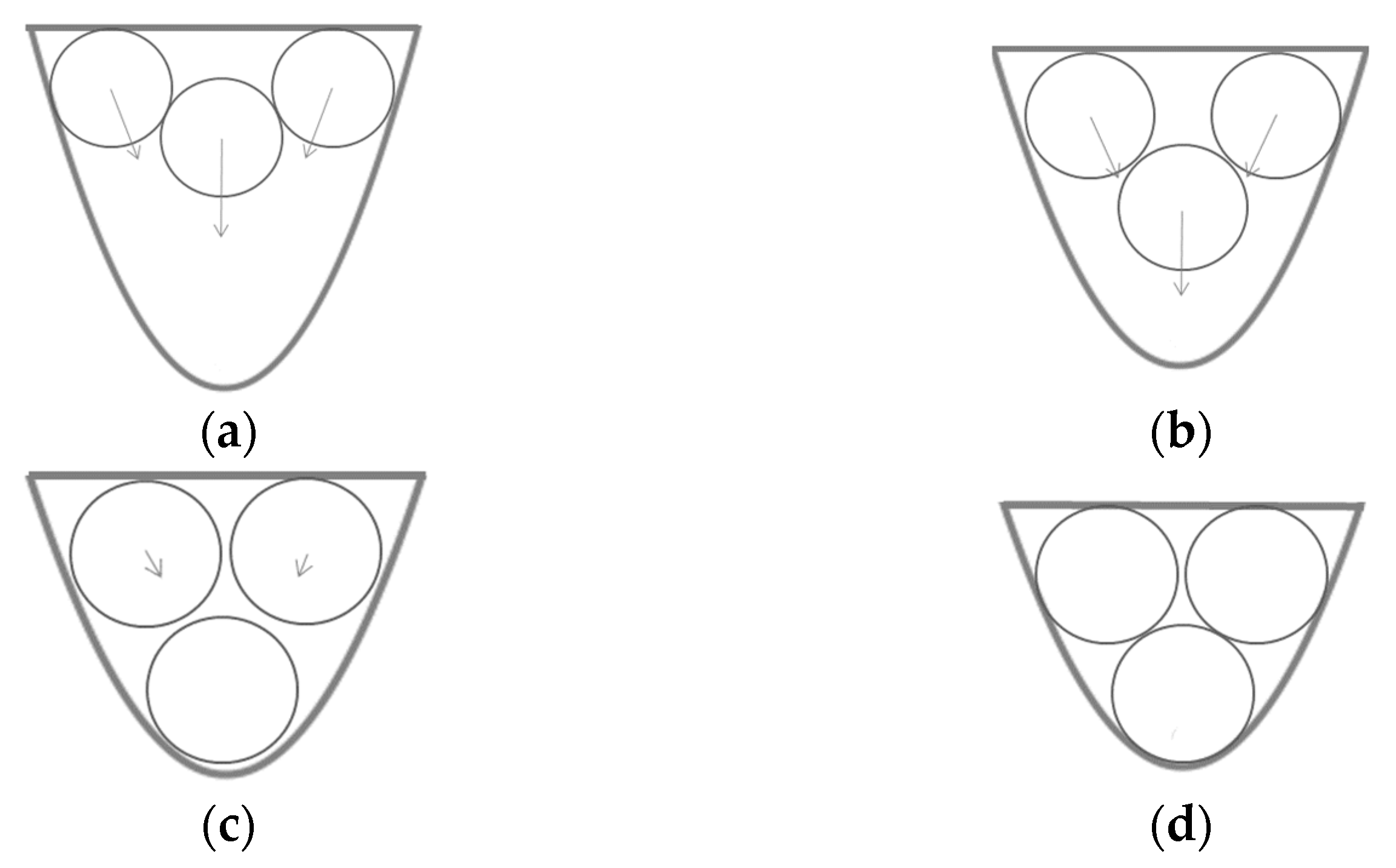
A schematic illustration of the proposed approach is shown in Figure 3. Three consecutive iterations of the FDM in 2D are illustrated in Figure 3a–c. An arrangement of 2D spheres corresponding to the stop criterion, $\Vert Y^{k+1}-Y^k\Vert <\tau$, at Step 11 is shown in Figure 3d.

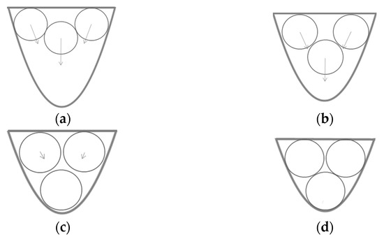
Figure 3. Illustration to the main stages of the solution procedure for three spheres: (a) an arrangement of spheres corresponding to the $k$-th iteration; (b) an arrangement of spheres corresponding to the $(k+1)$-th iteration; (c) an arrangement of spheres corresponding to the $(k+2)$-th iteration; (d) an arrangement of spheres corresponding to the stop criterion.

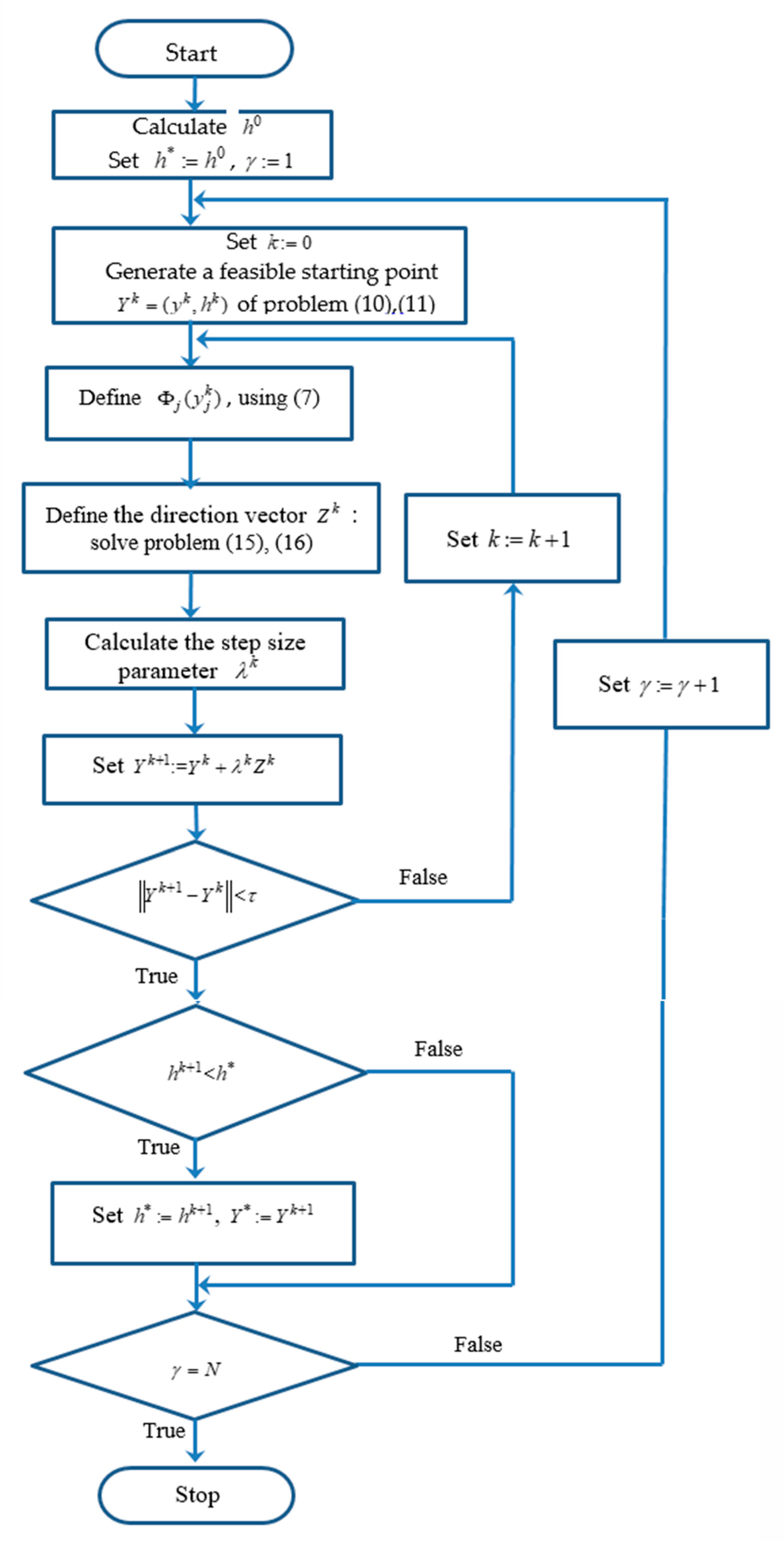
A flowchart corresponding to the solution strategy is presented in Figure 4.

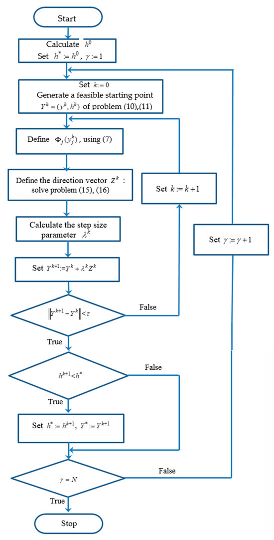
Figure 4. The flowchart of the main algorithm.

6. Computational Results

The proposed approach was numerically tested for eleven instances of the problem (9), (10) with different (a) dimensions, n = 2, 3, 4, 5; (b) numbers of spheres, m = 50, 100, 200; b) radii, $r_j,j=1,\dots ,m$; (c) minimal allowable distances, ${\delta }_{tj},{\delta }_j$, $t<j\in J$, $j\in J$; (d) parameters $p$ of the parabolic container, $p=1,2,5,10$. For all the examples, we set ${\epsilon }^0=\epsilon =1$, $\tau ={10}^{-6}$. For each problem instance, 10 starting points were generated. The computations were performed using an Intel^® Core™ i3-6100T, 3.20 GHz, 8.00 GB of RAM.

Example 1. $n=2$, $m=100$, $r_j=1.177$, $j=1,\dots ,24,$ $r_j=1.117$, $i=25,\dots ,48,$ $r_j=0.97$, $j=49,\dots ,72,$ $r_j=0.927$, $j=73,\dots ,96,$ $r_j=0.86$, $j=97,\dots ,100;$ $p=1$, ${\delta }_{tj}={\delta }_j=0$. The best solution found by our algorithm for 5 min is $h*=37.518079$.

Example 2. $n=2$, $m=200,$ $r_j=1.177$, $j=1,\dots ,24,$ $r_j=1.117$, $j=25,\dots ,48,$ $r_j=0.97$, $j=49,\dots ,72,$ $r_j=0.927$, $j=73,\dots ,96,$ $r_j=0.86$, $j=97,\dots ,120,$ $r_j=0.812$, $j=121,\dots ,144,$ $r_j=0.762$, $j=145,\dots ,168,$ $r_j=0.726$, $j=169,\dots ,192,$ $r_j=0.664$, $j=193,\dots ,200;$ $p=1$, ${\delta }_{tj}={\delta }_j=0$. The best solution found by our algorithm for 20 min is $h*=49.511450$.

Example 3. $n=2$, $m=100$, the radii are as in Example 1; $p=5$, ${\delta }_{tj}={\delta }_j=0$, $h^0=30$. The best solution found by our algorithm for 5 min is $h*=21.695951$.

Example 4. $n=2$, $m=50$, $\{r_j,j=1,\dots ,50\}=${1.177, 1.177, 1.177, 1.177, 1.117, 1.117, 1.117, 1.117, 1.117, 0.970, 0.970, 0.970, 0.970, 0.970, 0.927, 0.927, 0.927, 0.927, 0.927, 0.860, 0.860, 0.860, 0.860, 0.860, 0.812, 0.812, 0.812, 0.812, 0.812, 0.762, 0.762, 0.762, 0.762, 0.762, 0.726, 0.726, 0.726, 0.726, 0.726, 0.664, 0.664, 0.664, 0.664, 0.664, 0.627, 0.627, 0.627, 0.627, 0.627}, $p=5$, ${\delta }_{tj}\in [0.1,0.5]$, ${\delta }_j\in [0.1,1]$. The best solution found by our algorithm for 2 min is $h*=11.577099$.

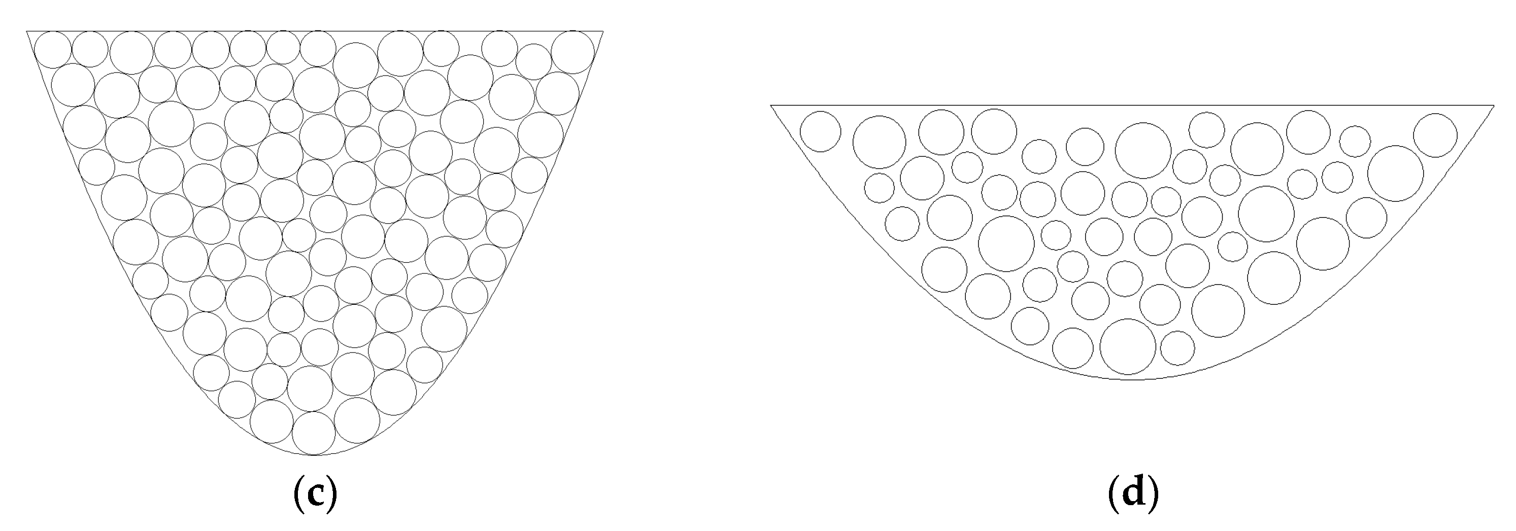
The corresponding placements of the spheres in Examples 1–4 are shown in Figure 5a–d.

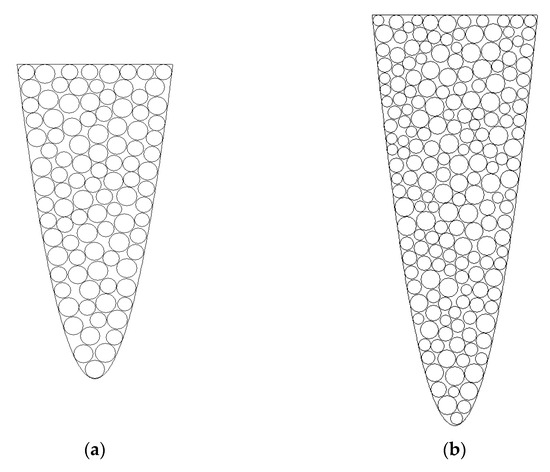
Figure 5. Optimized arrangement of 2D spheres: (a) Example 1; (b) Example 2; (c) Example 3; (d) Example 4.

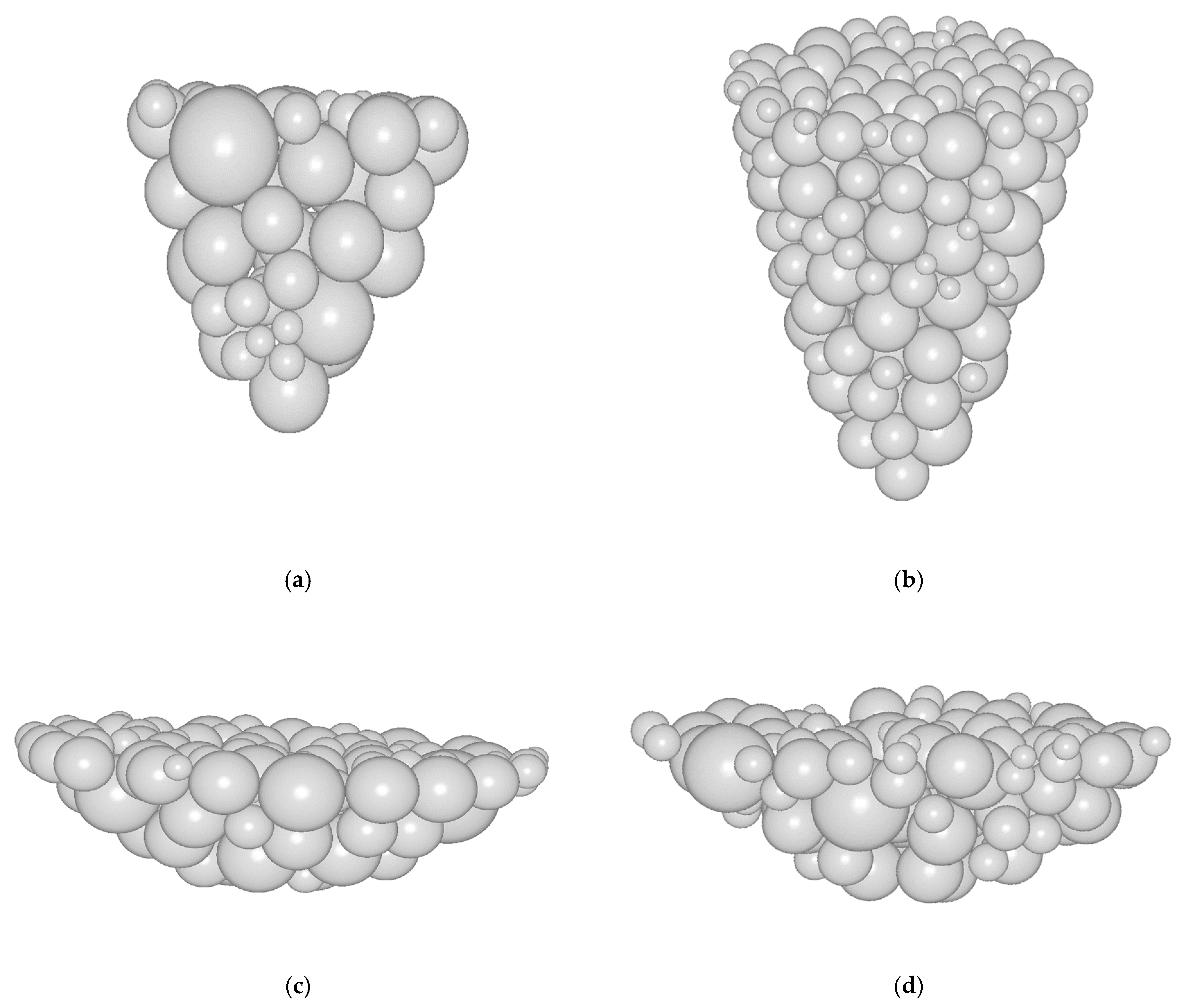
Example 5. $n=3$, $m=50$, $\{r_j,j=1,\dots ,50\}=${0.527, 0.564, 0.566, 0.592, 0.612, 0.680, 0.747, 0.760, 0.807, 0.845, 0.850, 0.853, 0.855, 0.868, 0.887, 0.891, 0.934, 0.947, 0.955, 0.961, 1.044, 1.085, 1.180, 1.189, 1.210, 1.229, 1.237, 1.274, 1.275, 1.281, 1.292, 1.309, 1.325, 1.374, 1.399, 1.404, 1.430, 1.484, 1.491, 1.493, 1.525, 1.551, 1.551, 1.636, 1.670, 1.739, 1.819, 2.050, 2.171}, $p=2$, ${\delta }_{tj}={\delta }_j=0$. The best solution found by our algorithm for 3 min is $h*=11.927860$.

Example 6. $n=3$, $m=200$, $\{r_j,j=1,\dots ,200\}=${2.171, 2.171, 2.171, 2.171, 2.050, 2.050, 2.050, 2.050, 1.819, 1.819, 1.819, 1.819, 1.739, 1.739, 1.739, 1.739, 1.670, 1.670, 1.670, 1.670, 1.636, 1.636, 1.636, 1.636, 1.551, 1.551, 1.551, 1.551, 1.551, 1.551, 1.551, 1.551, 1.525, 1.525, 1.525, 1.525, 1.493, 1.493, 1.493, 1.493, 1.491, 1.491, 1.491, 1.491, 1.484, 1.484, 1.484, 1.484, 1.484, 1.484, 1.484, 1.484, 1.430, 1.430, 1.430, 1.430, 1.404, 1.404, 1.404, 1.404, 1.399, 1.399, 1.399, 1.399, 1.374, 1.374, 1.374, 1.374, 1.325, 1.325, 1.325, 1.325, 1.309, 1.309, 1.309, 1.309, 1.292, 1.292, 1.292, 1.292, 1.281, 1.281, 1.281, 1.281, 1.275, 1.275, 1.275, 1.275, 1.274, 1.274, 1.274, 1.274, 1.237, 1.237, 1.237, 1.237, 1.229, 1.229, 1.229, 1.229, 1.210, 1.210, 1.210, 1.210, 1.189, 1.189, 1.189, 1.189, 1.180, 1.180, 1.180, 1.180, 1.085, 1.085, 1.085, 1.085, 1.044, 1.044, 1.044, 1.044, 0.961, 0.961, 0.961, 0.961, 0.955, 0.955, 0.955, 0.955, 0.947, 0.947, 0.947, 0.947, 0.934, 0.934, 0.934, 0.934, 0.891, 0.891, 0.891, 0.891, 0.887, 0.887, 0.887, 0.887, 0.868, 0.868, 0.868, 0.868, 0.855, 0.855, 0.855, 0.855, 0.853, 0.853, 0.853, 0.853, 0.850, 0.850, 0.850, 0.850, 0.845, 0.845, 0.845, 0.845, 0.807, 0.807, 0.807, 0.807, 0.760, 0.760, 0.760, 0.760, 0.747, 0.747, 0.747, 0.747, 0.680, 0.680, 0.680, 0.680, 0.612, 0.612, 0.612, 0.612, 0.592, 0.592, 0.592, 0.592, 0.566, 0.566, 0.566, 0.566, 0.564, 0.564, 0.564, 0.564, 0.527, 0.527, 0.527, 0.527}, $p=2$, ${\delta }_{tj}={\delta }_j=0$. The best solution found by our algorithm for 35 min is $h*=22.612047.$

Example 7. $n=3$, $m=100$, $\{r_j,j=1,\dots ,100\}=$ {2.171, 2.171, 2.050, 2.050, 1.819, 1.819, 1.739, 1.739, 1.670, 1.670, 1.636, 1.636, 1.551, 1.551, 1.551, 1.551, 1.525, 1.525, 1.493, 1.493, 1.491, 1.491, 1.484, 1.484, 1.484, 1.484, 1.430, 1.430, 1.404, 1.404, 1.399, 1.399, 1.374, 1.374, 1.325, 1.325, 1.309, 1.309, 1.292, 1.292, 1.281, 1.281, 1.275, 1.275, 1.274, 1.274, 1.237, 1.237, 1.229, 1.229, 1.210, 1.210, 1.189, 1.189, 1.180, 1.180, 1.085, 1.085, 1.044, 1.044, 0.961, 0.961, 0.955, 0.955, 0.947, 0.947, 0.934, 0.934, 0.891, 0.891, 0.887, 0.887, 0.868, 0.868, 0.855, 0.855, 0.853, 0.853, 0.850, 0.850, 0.845, 0.845, 0.807, 0.807, 0.760, 0.760, 0.747, 0.747, 0.680, 0.680, 0.612, 0.612, 0.592, 0.592, 0.566, 0.566, 0.564, 0.564, 0.527, 0.527}, $p=10$, ${\delta }_{tj}={\delta }_j=0$, $h^0=40$. The best solution found by our algorithm for 10 min is $h*=7.577422$.

Example 8. $n=3$, $m=100$, the radii are as in Example 7; $p=10$, ${\delta }_{tj}\in [0.1,0.5]$, ${\delta }_j\in [0.1,1]$. The best solution found by our algorithm for 10 min is $h*=9.727001$.

The corresponding placements of the 3D spheres in Examples 5–8 are shown in Figure 6a–d.

Figure 6. Optimized arrangement of 3D spheres: (a) Example 5; (b) Example 6; (c) Example 7; (d) Example 8.

Example 9. $n=4$, $m=100$, the radii are as in Example 7; $p=2$, ${\delta }_{tj}={\delta }_j=0$. The best solution found by our algorithm for 15 min is $h*=22.612047$.

Example 10. $n=4$, $m=200$, the radii are as in Example 6; $p=2$, ${\delta }_{tj}={\delta }_j=0$. The best solution found by our algorithm for 45 min is $h*=14.628068$.

Example 11. $n=4$, $m=200$, the radii are as in Example 6; $p=2$, ${\delta }_{tj}={\delta }_j=0$. The best solution found by our algorithm for 55 min is $h*=11.791466$.

7. Conclusions

Employing mathematical models offers a structured and systematic approach to problem-solving, facilitating precise analysis and prediction of outcomes [32]. In this paper, a mathematical model for packing different spheres into a minimal-height parabolic container is proposed. Non-overlapping and containment conditions are formulated using the phi-function approach. The minimal allowed distance between the spheres and the boundary of the container is considered. The problem belongs to a class of irregular packing problems due to the nonstandard container shape.

To solve the corresponding nonlinear optimization problem, a feasible directions approach combined with the hot start technique is proposed. A decomposition scheme is applied to reduce the number of constraints in the subproblem used to find the search direction. Numerical experiments are provided to demonstrate the efficiency of the proposed solution scheme. A detailed description of the problem instances and corresponding solutions are reported to form a benchmark for future research.

Our future research is focused on the following issues. The number of non-overlapping constraints grows quadratically with an increase in the number of spheres, resulting in a large-scale optimization problem. These constraints have a specific structure which can be used either for direct solution of the original problem or to construct tight bounds for the optimal objective [33,34]. The proposed approach is based on modeling the interactions between the spheres and the boundary of the parabolic container. It also can be applied to a broader class of containers, e.g., circular hyperboloids (single- and double-sheeted), spheroids or ellipsoids. Packing problems on surfaces [35] can also be considered, as well as various applications of spherical systems [36] and logistics [37]. Some results in these directions are forthcoming.

References

- Scheithauer, G. Introduction to Cutting and Packing Optimization. In International Series in Operations Research & Management Science; Springer: Cham, Switzerland, 2018; Volume 263, pp. 385–405. [Google Scholar] [CrossRef]
- Wäscher, G.; Haußner, H.; Schumann, H. An improved typology of cutting and packing problems. Eur. J. Oper. Res. 2007, 183, 1109–1130. [Google Scholar] [CrossRef]
- Castillo, I.; Kampas, F.J.; Pinter, J.D. Solving circle packing problems by global optimization: Numerical results and industrial applications. Eur. J. Oper. Res. 2008, 191, 786–802. [Google Scholar] [CrossRef]
- Kampas, F.J.; Castillo, I.; Pinter, J.D. Optimized ellipse packings in regular polygons. Optim. Lett. 2019, 13, 1583–1613. [Google Scholar] [CrossRef]
- Kallrath, J.; Rebennack, S. Cutting ellipses from area-minimizing rectangles. J. Glob. Optim. 2014, 59, 405–437. [Google Scholar] [CrossRef]
- Pankratov, A.; Romanova, T.; Litvinchev, I. Packing ellipses in an optimized rectangular container. Wirel. Netw. 2020, 26, 4869–4879. [Google Scholar] [CrossRef]
- Kampas, F.J.; Pintér, J.D.; Castillo, I. Packing ovals in optimized regular polygons. J. Glob. Optim. 2020, 77, 175–196. [Google Scholar] [CrossRef]
- Castillo, I.; Pintér, J.D.; Kampas, F.J. The boundary-to-boundary p-dispersion configuration problem with oval objects. J. Oper. Res. Soc. 2024, 1–11. [Google Scholar] [CrossRef]
- Elser, V. Packing spheres in high dimensions with moderate computational effort. Phys. Rev. E 2023, 108, 034117. [Google Scholar] [CrossRef] [PubMed]
- Litvinchev, I.; Fischer, A.; Romanova, T.; Stetsyuk, P. A new class of irregular packing problems reducible to sphere packing in arbitrary norms. Mathematics 2024, 12, 935. [Google Scholar] [CrossRef]
- Kallrath, J. Packing ellipsoids into volume-minimizing rectangular boxes. J. Glob. Optim. 2017, 67, 151–185. [Google Scholar] [CrossRef]
- Leao, A.A.S.; Toledo, F.M.B.; Oliveira, J.F.; Carravilla, M.A.; Alvarez-Valdes, R. Irregular packing problems: A review of mathematical models. Eur. J. Oper. Res. 2020, 282, 803–822. [Google Scholar] [CrossRef]
- Guo, B.; Zhang, Y.; Hu, J.; Li, J.; Wu, F.; Peng, Q.; Zhang, Q. Two-dimensional irregular packing problems: A review. Front. Mech. Eng. 2022, 8, 966691. [Google Scholar]
- Rao, Y.; Luo, Q. Intelligent algorithms for irregular packing problem. In Intelligent Algorithms for Packing and Cutting Problem; Engineering Applications of Computational Methods; Springer: Singapore, 2022; Volume 10. [Google Scholar] [CrossRef]
- Lamas-Fernandez, C.; Bennell, J.A.; Martinez-Sykora, A. Voxel-based solution Aapproaches to the three-dimensional irregular packing problem. Oper. Res. 2023, 71, 1298–1317. [Google Scholar] [CrossRef]
- Gil, M.; Patsuk, V. Phi-functions for objects bounded by the second-order curves and their application to packing problems. In Smart Technologies in Urban Engineering; Arsenyeva, O., Romanova, T., Sukhonos, M., Tsegelnyk, Y., Eds.; STUE 2022, Lecture Notes in Networks and Systems; Springer: Cham, Switzerland, 2023; Volume 536. [Google Scholar] [CrossRef]
- Santini, C.; Mangini, F.; Frezza, F. Apollonian Packing of Circles within Ellipses. Algorithms 2023, 16, 129. [Google Scholar] [CrossRef]
- Amore, P.; De la Cruz, D.; Hernandez, V.; Rincon, I.; Zarate, U. Circle packing in arbitrary domains featured. Phys. Fluids 2023, 35, 127112. [Google Scholar] [CrossRef]
- Kovalenko, A.A.; Romanova, T.E.; Stetsyuk, P.I. Balance Layout Problem for 3D-Objects: Mathematical Model and Solution Methods. Cybern. Syst. Anal. 2015, 51, 556–565. [Google Scholar] [CrossRef]
- Burtseva, L.; Pestryakov, A.; Romero, R.; Valdez, B. Petranovskii. Some aspects of computer approaches to simulation of bimodal sphere packing in material engineering. Adv. Mater. Res. 2014, 1040, 585–591. [Google Scholar] [CrossRef]
- Ungson, Y.; Burtseva, L.; Garcia-Curiel, E.R.; Valdez Salas, B.; Flores-Rios, B.L.; Werner, F.; Petranovskii, V. Filling of Irregular Channels with Round Cross-Section: Modeling Aspects to Study the Properties of Porous Materials. Materials 2018, 11, 1901. [Google Scholar] [CrossRef] [PubMed]
- Burtseva, L.; Valdez Salas, B.; Romero, R.; Werner, F. Recent advances on modelling of structures of multi-component mixtures using a sphere packing approach. Int. J. Nanotechnol. 2016, 13, 44–59. [Google Scholar] [CrossRef]
- Available online: https://olofly.com/product/huni-badger-parabolic-dish-container/ (accessed on 7 April 2023).
- Chernov, N.; Stoyan, Y.; Romanova, T. Mathematical model and efficient algorithms for object packing problem. Comput. Geom. Theory Appl. 2010, 43, 535–553. [Google Scholar] [CrossRef]
- Nocedal, J.; Wright, S.J. Numerical Optimization; Springer Series in Operations Research and Financial Engineering; Springer: New York, NY, USA, 2006. [Google Scholar]
- Kallrath, J. Business Optimization Using Mathematical Programming; Springer: London, UK, 2021; ISBN 978-3-030-73237-0. [Google Scholar]
- Chen, D. Sphere Packing Problem. In Encyclopedia of Algorithms; Kao, M.Y., Ed.; Springer: Boston, MA, USA, 2008. [Google Scholar] [CrossRef]
- Sahinidis, N. BARON User Manual v. 2024.5.8. Available online: https://minlp.com/downloads/docs/baron%20manual.pdf (accessed on 8 May 2024).
- IPOPT: Documentation. Available online: https://coin-or.github.io/Ipopt/ (accessed on 14 January 2023).
- Stoyan, Y.; Yaskov, G. Packing congruent hyperspheres into a hypersphere. J. Glob. Optim. 2012, 52, 855–868. [Google Scholar] [CrossRef]
- Romanova, T.; Stoyan, Y.; Pankratov, A.; Litvinchev, I.; Marmolejo, J.A. Decomposition algorithm for irregular placement problems. In Intelligent Computing and Optimization, Proceedings of the 2nd International Conference on Intelligent Computing and Optimization 2019 (ICO 2019), Koh Samui, Thailand, 3–4 October 2019; Intelligent Systems and Computing; Springer: Cham, Switzerland, 2019; Volume 1072, pp. 214–221. [Google Scholar]
- Animasaun, I.L.; Shah, N.A.; Wakif, A.; Mahanthesh, B.; Sivaraj, R.; Koriko, O.K. Ratio of Momentum Diffusivity to Thermal Diffusivity: Introduction, Meta-Analysis, and Scrutinization; Chapman and Hall/CRC: New York, NY, USA, 2022. [Google Scholar] [CrossRef]
- Litvinchev, I.S. Refinement of Lagrangian bounds in optimization problems. Comput. Math. Math. Phys. 2007, 47, 1101–1108. [Google Scholar] [CrossRef]
- Litvinchev, I.; Rangel, S.; Saucedo, J. A Lagrangian bound for many-to-many assignment problems. J. Comb. Optim. 2010, 19, 241–257. [Google Scholar] [CrossRef]
- Lai, X.; Yue, D.; Hao, J.K.; Glover, F.; Lü, Z. Iterated dynamic neighborhood search for packing equal circles on a sphere. Comput. Oper. Res. 2023, 151, 106121. [Google Scholar] [CrossRef]
- Asadi Jafari, M.H.; Zarastvand, M.; Zhou, J. Doubly curved truss core composite shell system for broadband diffuse acoustic insulation. J. Vib. Control 2023. [Google Scholar] [CrossRef]
- Bulat, A.; Kiseleva, E.; Hart, L.; Prytomanova, O. Generalized Models of Logistics Problems and Approaches to Their Solution Based on the Synthesis of the Theory of Optimal Partitioning and Neuro-Fuzzy Technologies. In System Analysis and Artificial Intelligence; Studies in Computational Intelligence; Zgurovsky, M., Pankratova, N., Eds.; Springer: Cham, Switzerland, 2023; Volume 1107, pp. 355–376. [Google Scholar] [CrossRef]
Disclaimer/Publisher’s Note: The statements, opinions and data contained in all publications are solely those of the individual author(s) and contributor(s) and not of MDPI and/or the editor(s). MDPI and/or the editor(s) disclaim responsibility for any injury to people or property resulting from any ideas, methods, instructions or products referred to in the content. |
© 2024 by the authors. Licensee MDPI, Basel, Switzerland. This article is an open access article distributed under the terms and conditions of the Creative Commons Attribution (CC BY) license (https://creativecommons.org/licenses/by/4.0/).