Abstract
This paper introduces an iterative method with a remarkable level of accuracy, namely fourth-order convergence. The method is specifically tailored to meet the optimality condition under the Kung–Traub conjecture by linear combination. This method, with an efficiency index of approximately , employs a blend of localized and semi-localized analysis to improve both efficiency and convergence. This study aims to investigate semi-local convergence, dynamical analysis to assess stability and convergence rate, and the use of the proposed solver for systems of nonlinear equations. The results underscore the potential of the proposed method for several applications in polynomiography and other areas of mathematical research. The improved performance of the proposed optimal method is demonstrated with mathematical models taken from many domains, such as physics, mechanics, chemistry, and combustion, to name a few.
MSC:
65H05; 41A25; 28A80; 46N40
1. Introduction
Root-finding methods are essential in various scientific disciplines for solving nonlinear systems, which are systems of equations that cannot be represented as linear combinations of their inputs. These techniques, which include Newton’s method, the bisection method, and the secant method, are used to determine solutions to equations where the function is zero, called [1] roots. Engineering relies on the use of equations to address the qualities of materials and forces, which are crucial to the design of systems and structures. In the field of physics, differential equations are used to elucidate various phenomena related to motion, energy, and waves. Root-finding algorithms are used in finance to calculate the internal rate of return and in option pricing models [2]. These methods are necessary because nonlinear systems are very complicated and often cannot be solved analytically or need to be greatly simplified in order to be solved. Root-finding methods provide an accurate numerical approach to approximate answers with a high level of accuracy. This allows scientists and engineers to effectively model real-world phenomena, optimize systems, and make predictions based on theoretical models.
As mentioned above, iterative root-finding algorithms are essential computational methods used to solve equations in which a function is equal to zero, demonstrated as follows:
Equations of the (1) type are of utmost importance in the fields of mathematics, engineering, physics, and computer science. They are employed to tackle a wide range of problems, including the optimization of engineering designs and the solution of equations in theoretical physics, among others [3,4].
There exists a continuous operator, , in Equation (1). This operator is defined on a nonempty convex subset D of a Banach space S and has values in a Banach space . This investigation aims to determine an approximation of the unique local solution for the problem stated in (1). In the one-dimensional example, Banach spaces are equivalent to . The problem can be reduced to approximating a single local root of
where and I is a neighborhood of [5].
An essential objective of the numerical analysis is to find the origin of nonlinear equations, whether they are single-variable or multivariable. This endeavor has led to the development of multiple algorithms that strive to predict exact solutions with the required level of accuracy. The pursuit of accuracy and efficiency in solving complex equations drives the advancement and application of iterative methods for root determination. Numerical methods play a crucial role in practical situations where it is often impossible to obtain accurate results by analytical means. Moreover, the ability to quickly and accurately determine the solutions of nonlinear equations is crucial in simulations, optimizations, and modeling in various scientific fields, making these techniques indispensable tools for researchers [6,7]. The main numerical analysis techniques are the bisection method, the Newton–Raphson method, and the secant method. The bisection method is a reliable, albeit slow, strategy that guarantees convergence by halving the interval containing the root at each iteration. In contrast, the Newton–Raphson method offers a higher convergence rate by using the derivative of the function, making it a preferable technique for many applications requiring speed and efficiency. The derivative-free secant method offers a middle ground between the bisection and Newton–Raphson methods. It provides an efficient method that does not depend heavily on the differentiability of the function.
Recent studies have led to the development of sophisticated algorithms, such as two- and three-step root-finding approaches, which aim to improve convergence rates and stability [8,9,10,11,12]. These methods improve traditional iterative algorithms by incorporating additional steps or using higher-order derivatives to improve accuracy and speed. For example, two-step methods typically involve an initial Newton–Raphson-like step followed by a corrective phase that improves the accuracy of the root computation. Three-step techniques improve on this idea by introducing an additional level of precision, whereby even higher levels of accuracy can be achieved. Discussions on the optimality of root-finding algorithms revolve mainly around their speed of convergence and computational efficiency. Second-order algorithms, such as the improved Newton–Raphson methodology and some variants of the secant method, offer a practical balance between computational simplicity and fast convergence.
In contrast, fourth-order convergent methods aim to achieve faster convergence at the expense of computational simplicity, as they require higher-order derivatives or additional function evaluations. These approaches are especially valuable for solving complex equations that require fast convergence and are not limited by processing resources. Iterative methods used in numerical analysis to find the roots of nonlinear equations are essential, as they allow for solving otherwise intractable problems. The progression of these algorithms, ranging from traditional textbook approaches to the latest research advances, demonstrates the continuing quest for greater efficiency, accuracy, and practicality. As computing power increases, root-finding algorithms will also improve in sophistication and performance, underscoring their continuing importance in mathematics and the sciences. This summary provides insight into the thorough and precise analysis needed to fully understand and appreciate the breadth and variety of iterative root-finding methods. The original question requires a thorough examination of the subject, including such aspects as theoretical foundations, improvements in algorithms, comparative evaluations of methodologies, and discussions of practical implementations and applications. Engaging in such a task would require a substantial document, which exceeds the brief summary provided here.
2. Existing Optimal Algorithms
The Kung–Traub conjecture [13], introduced in the 1970s, establishes a theoretical upper bound on the effectiveness of iterative techniques used to solve nonlinear equations. According to this hypothesis, the highest convergence order of any iterative root-finding algorithm employing a finite number of function evaluations per iteration is , where d is the number of derivative evaluations per iteration. Essentially, this implies that for methods that do not compute derivatives (i.e., ), such as the bisection method, the order of convergence is 1 (linear convergence). The maximum order of convergence for methods that evaluate the function and its first derivative (i.e., when , such as Newton’s method) is 2. The conjecture establishes a standard for judging how well algorithms for finding roots perform: the Kung–Traub framework says that an optimal algorithm for finding roots achieves the highest possible level of convergence as a function of the number of derivative evaluations it performs. As a result, several algorithms have been created to achieve these efficiency bounds, including Halley’s approach and other advanced methods. As defined by Kung and Traub, these algorithms attempt to strike a balance between computational cost and convergence speed.
Newton’s method is one of the classical optimal methods for solving equations of the type (2), with the following computational steps:
where The optimal second-order convergent solver given in (3) requires only two function evaluations per iteration.
The optimal two-step fourth-order convergent solver (OPNM1) in [14] is given by the following computational steps:
The numerical solver (4) requires, at each iteration, three function evaluations ( and two evaluations of the first-order derivative and ).
In the same research article [14], the authors proposed another optimal two-step fourth-order convergent solver (OPNM2), which is given by the following computational steps:
The numerical solver (5) also requires, at each iteration, three function evaluations ( and two evaluations of the first-order derivative and ).
Jaiswal [15] proposed an optimal two-step fourth-order convergent solver (OPNM3), which is given by the following computational steps:
Once again, the numerical solver (6) requires, at each iteration, three function evaluations ( and two evaluations of the first-order derivative and ).
In the same research paper [15], Jaiswal also proposed a second optimal two-step fourth-order convergent solver (OPNM4), which is given by the following computational steps:
Once again, the numerical solver (7) requires, at each iteration, three function evaluations ( and two evaluations of the first-order derivative, and ).
There are several fourth-order optimal numerical solvers for solving nonlinear equations, both univariate and multivariate. However, it is crucial to note that several recently suggested optimal techniques are not suitable for solving nonlinear equations in higher dimensions. The optimal methods, devised in [16,17,18,19], do not usually attempt to be used for nonlinear systems, whereas the fourth-order optimal method proposed in the present research study solves both scalar and vector versions of nonlinear equations.
3. Construction of the Optimal Fourth-Order Numerical Solver
In this section, we use the notion of a linear combination of two well-established third-order (non-optimal) numerical solvers to obtain an optimal numerical solver for dealing with nonlinear equations of the type (1). Both numerical solvers, chosen for the linear combination, are discussed in [14] and given as follows:
and
where and
Our major aim is to construct a fourth-order optimal convergent numerical solver using a linear combination of solvers given in (8) and (9). The linear combination has the following form:
where is the adjusting parameter. When , the method reduces to (8), while results in (9). Methods given in (8) and (9) are not optimal, while (10) is an optimal fourth-order convergent solver for a suitable choice of . The performance of (10) depends on the adjustment parameter which is obtained from the Taylor expansion as given in Theorem 1.
Theorem 1.
Assume that the function has a simple root , where D is an open interval. If φ is sufficiently smooth in the neighborhood of the root α, then the order of convergence of the iterative method defined by (10) is at least three, as shown in the following equation:
where , and , . Furthermore, if , then the order of convergence is four.
Proof of Theorem 1.
Let and .
Expanding via a Taylor series expansion around , we have the following:
Expanding via a Taylor series expansion around , we have the following:
Expanding via a Taylor series expansion around , we have the following:
Dividing (12) by (13), we have the following:
Substituting (15) in the first step of (20), gives the following:
where .
Expanding via a Taylor series expansion around and using Equation (16), we have the following:
Expanding via a Taylor series expansion around and using Equation (16), gives the following:
Finally, substituting the obtained series obtained in (12), (14), (17), and (18) into the structure defined in (10), the error equation is obtained as follows:
To increase the convergence order of (10), the error equation, Equation (19), suggests that the parameter should be . Using this value of in (10), the proposed optimal numerical method (OPPNM) takes the following form:
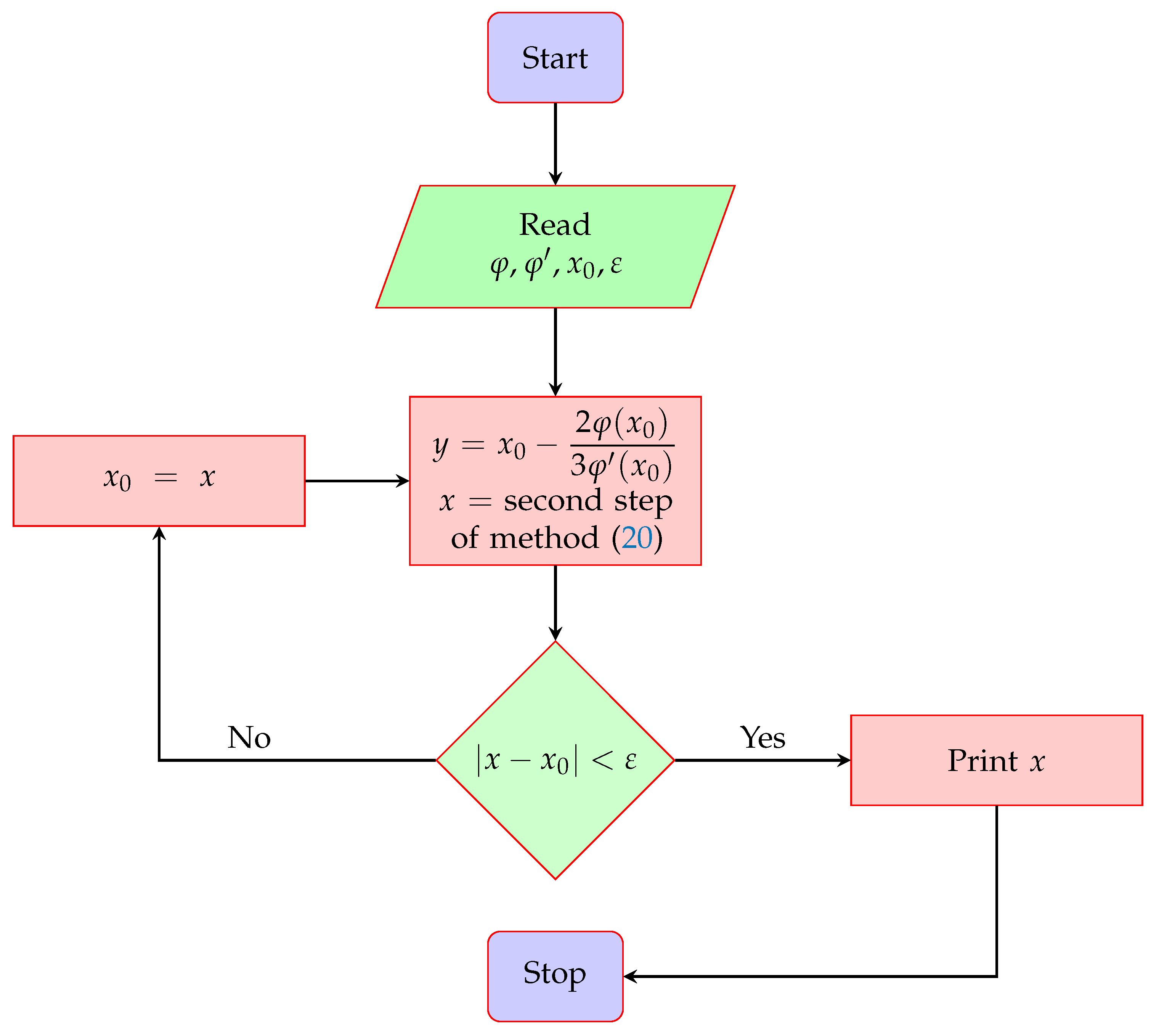
where . Numerical solver (20) is optimal under the Kung–Traub conjecture since its order of convergence equals , where represents the number of function evaluations taken by the solver at each iteration. The proposed numerical solver uses three function evaluations (one function evaluation and two of its first-order derivatives) at each iteration and has fourth-order local convergence, which is also discussed in the next section. The flowchart of the proposed two-step optimal numerical solver is shown in Figure 1.
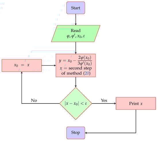
Figure 1.
Flowchart of the proposed optimal fourth-order numerical solver given in (20).
4. Local Convergence Analysis
4.1. Scalar Form
Local convergence analysis is a method used to determine the specific conditions under which a given iterative procedure can effectively converge to a solution of a nonlinear equation of the form (1). More specifically, it calculates the region of the complex plane encompassing a root into which the iterative method will converge. The study begins by assuming that the iterative method has achieved convergence at a root and then investigates the behavior of the procedure at that root. The analysis usually consists of examining the behavior of the iteration function of the method, which establishes a connection between the current approximation of the root and the subsequent approximation. Taylor series expansion is an essential tool for performing local convergence analysis. It allows us to estimate the iteration function in the vicinity of the root. Consequently, this estimation can be used to determine the rate at which the strategy reaches the root, as well as the conditions that must be satisfied for convergence.
The study usually involves determining the radius of convergence, which is the distance from the root that the iteration function can be approximated by a Taylor series expansion. The iterative approach guarantees convergence to the root if the initial estimate is within the radius of convergence. The root-finding methods usually examined by local convergence analysis are Newton’s method, the secant method, and the bisection method. By analyzing the behavior of these solutions, one can determine their strengths and weaknesses and identify the scenarios in which they are most effective. Therefore, our objective is to examine the local convergence of the suggested numerical solver (20) employing Taylor series expansion. This requires us to give the following theorem:
Theorem 2.
Suppose that is the exact root of a differentiable function for an open interval Then, the two-step method given in (20) has fourth-order convergence, and the asymptotic error term is determined to be
where and ,
4.2. Vector Form
The suggested method is optimal and can be used effectively for both single-variable and multivariable problems while maintaining simplicity. Within this particular framework, the approach uses the Jacobian matrix, which covers all first-order partial derivatives of the system, to progressively estimate the solution of the system through iterations. The approach starts with an initial estimation of the solution and then performs corrections at each step. These corrections are generated by multiplying the inverse of the Jacobian matrix by two-thirds of the vector of negative functions evaluated in the current estimate. The process is carried out for the second step in the suggested method. The iterative procedure persists until the solution reaches a state in which it satisfies the system of equations within a preset tolerance. This approach effectively handles the intricate nonlinear relationships between variables. This scheme is highly appreciated for its fast convergence and accuracy in various scientific and technical applications, provided that the initial approximation is close enough to the real solution and the system satisfies specific constraints on the invertibility of the Jacobian.
Let us formalize the approach to discuss the proposed optimal method (20) for solving a system of nonlinear equations. Let us consider a system of n nonlinear equations with n variables, represented as follows:
where is a vector-valued function of , and each is a nonlinear function of the variables .
The method seeks to find a vector , such that . Starting from an initial guess , the method iteratively updates the estimate of the root using the following formula:
where is the Jacobian matrix of evaluated at , and n is the iteration index. The Jacobian matrix is defined as follows:
The method applies a correction that is expected to bring the current estimate closer to the true solution by solving a linear system at each iteration. The process is repeated until a convergence criterion is met, such as when the norm of the function vector is less than a specified tolerance, indicating that is close to the root.
Many things affect how quickly the optimal solver (20) converges locally. These include the quality of the initial approximation and the Jacobian matrix’s properties. Given favorable circumstances, the approach exhibits quartic convergence, greatly enhancing its efficiency in solving nonlinear systems. Nevertheless, if the Jacobian matrix is singular or nearly unique during any iteration, the approach may either fail to converge or converge to a solution that does not satisfy the given system.
Here, we present the results to demonstrate the error equation and, consequently, the order of convergence of the proposed strategy for a system of nonlinear equations.
Lemma 1
([20]). Let be an r-times Fréchet differentiable in a convex set . Then, for any and , the following expression holds:
where
and the symbol means .
We introduce the following theorem to demonstrate the error equation and, consequently, the convergence order for the proposed optimal solver while dealing with a system of nonlinear equations, as follows:
Theorem 3
([21]). Let the function be sufficiently differentiable in a convex set Θ containing a simple zero α of . Let us consider that is continuous and nonsingular in α. If the initial guess is close to α, then the sequence obtained with the proposed two-step optimal solver (23) converges to α with fourth-order convergence.
Proof of Theorem 3.
Let be the root of , be the nth approximation to the root by (23), and be the error vector after the nth iteration. Expanding via a Taylor series expansion around , we obtain the following:
where
Expanding via a Taylor series expansion around gives the following:
Expanding via a Taylor series expansion around leads to the following:
Multiplying (25) and (27), we have the following:
Substituting (28) in the first step of (20) yields the following:
where . Expanding via a Taylor series expansion around and using Equation (29), we have the following:
Expanding via a Taylor series expansion around and using Equation (29),
Now, substituting Equations (25)–(27), (30), and (31) in the second step of (23), the error equation is obtained as follows:
Error Equation (32) proves the fourth-order convergence of the proposed two-step optimal method (23) presented in the vector form. □
5. Convergence without Taylor Series
Semi-local convergence for the proposed solver (20) requires a careful balance between the proximity of the initial approximation to the root, the behavior of the function and its derivatives near the root, and the inherent properties of the solver. By establishing the necessary conditions on the function and the initial approximation, and by a detailed analysis of the error dynamics, it can be seen that the solver exhibits fourth-order convergence within a certain neighborhood around the root. This analysis not only guarantees the effectiveness of the solver but also provides practical guidance on its application for solving equations where high accuracy is desired.
There are some problems with the Taylor series methodology employed to show local convergence analysis for the (20) solver limiting its applicability even though convergence is possible. We list these problems as follows:
- (P1)
- The local convergence is carried out for functions on the real line or the finite-dimensional Euclidean space.
- (P2)
- The function must be at least five times differentiable. Let us consider a function , defined as follows:where and Then, is a solution of the equation . But the function is not continuous at Thus, the results of the previous section—being only sufficient—cannot guarantee the convergence of the sequence generated by the method to the solution . However, the method converges to if, for example, we start from . This observation indicates that the sufficient convergence conditions can be weakened.
- (P3)
- There is no a priori knowledge of the number of iterations required to reach a desired error tolerance since no computable upper bounds on are given.
- (P4)
- The separation of the solutions is not discussed.
- (P5)
- The semi-local analysis of convergence, which is considered to be more important, is not considered either.
We positively address the above-listed problems (P1)–(P5) as follows:
- (P1)’
- The convergence analysis is carried out for Banach space-valued operators.
- (P2)’
- Both types of analyses use conditions only on the operators on the method (20).
- (P3)’
- The number of iterations to reach the error tolerance is known in advance since priori estimates on are provided.
- (P4)’
- The separation of the solutions is discussed.
- (P5)’
- The semi-local analysis of convergence relies on majorizing sequences [22,23]. These analyses also depend on control by generalized continuity conditions. This approach allows us to extend the utilization of the method (20).
Let denote Banach spaces, denote a convex, non-empty set that is open or closed, and denote a differentiable operator in the sense of Fréchet. We shall locate a solution of the equation iteratively. In particular, method (20) is utilized in the setting, and is defined for and each by the following:
It is clear that the method (33) reduces to (20) if (j is a natural number).
5.1. Local Analysis of Convergence
The conditions are for Suppose we have the following:
- (C1)
- There exists the smallest solution of the equation where is a continuous and non-decreasing function. Set
- (C2)
- There exists a function, , such that is defined by the following:the equation has the smallest solution in the interval denoted as .
- (C3)
- The equation where is defined byhas the smallest solution , denoted as Set and
- (C4)
- The equation where is defined by the following:has the smallest solution in denoted as Set
- (C5)
- There exists and a solution such that so that for each , Set .
- (C6)
- for each and
- (C7)
- .
Under the conditions (C1)–(C7), we present the local analysis of convergence for the method (33).
Theorem 4.
Suppose that the conditions (C1)–(C7) hold. Then, the following assertions hold for the iterates produced by the method (33) provided that
and the sequence converges to the solution γ of the equation
Proof of Theorem 4.
Let Then, the application of the conditions (C1), (C5), and (34) imply for
Thus, the Banach Lemma involving inverses of linear operators assures [22,23] that as well as
It also follows that the iterate exists by the first substep of the method (33) if
Using (34), (C6), (38), and (39), we have the following in turn:
So assertion (36) holds if and iterate . As in (38), we have the following:
so and
Consequently, the iterate exists by the second substep of the method (33), and
Leading by (34), (40), (38), (41), (C1), and (C6) that
Thus, the assertion (37) holds if and the iterate By switching by (m a natural integer), we terminate the induction for the assertions (35)–(37). Then, the estimation
where shows that . □
Remark 1.
- (i)
- The radius r in the condition (C7) can be replaced by
- (ii)
- Possible choices of the operator Δ can be or , provided that the operator is invertible. Other choices are possible, as long as conditions (C5) and (C6) hold.
The separation of the solutions is developed in the following result.
Proposition 1.
Suppose there exists , such that the condition (C5) holds in the ball , and there exists , such that we have the following:
Set Then, the equation is uniquely solvable by γ in the set
Proof.
Proof of Proposition 1 Suppose that there exists such that , and Define the linear operator Then, it follows by (C5) and (45) that
Then, and from the following approximation,
Consequently, we can conclude that □
Remark 2.
We can certainly choose in Proposition 1.
5.2. Semi-Local Analysis of Convergence
The roles of , and are exchanged by and as follows. Suppose that we have the following:
- (H1)
- Equation has the smallest solution denoted by in the interval where is a continuous as well as a non-decreasing function. Set
- (H2)
- There exists a function , which is continuous as well as non-decreasing. We define the sequence for some and each by the following:The scalar sequence , as defined, is shown in Theorem 4 to be majorizing for the method (33). But first, a general convergence condition for it is needed.
- (H3)
- There exists , such that for each andIt follows by simple induction (46) and condition (H3) that . Thus, the real sequence is nondecreasing and bounded from above by , and as such, it is convergent to some such that .The limit is the unique least upper bound of the sequence . Notice that if is strictly increasing, we can take As in the local analysis, the functions and relate to the operators of the method (33).
- (H4)
- There exists an invertible operator such that for some ,Set Notice that for , we have Thus, and we can take
- (H5)
- for each , and
- (H6)
The semi-local analysis relies on the conditions (H1)–(H6).
Theorem 5.
Suppose that the conditions (H1)–(H6) hold. Then, it follows that assertions hold for the sequence produced by the method (33).
and there exists a solution of the equation , so that
Proof of Theorem 5.
As in the local analysis, the assertions (47)–(49) are shown using induction. The definition of , and the first substep of the method (33) imply that the assertions (47) and (48) hold for and iterate . The conditions (H1)–(H4), in the local case, show the following:
so and , and similarly
so , and
Consequently, the iterate exists by the second substep of the method (33). By subtracting the first from the second substep of the method (33), we have the following:
and
so the assertion (47) holds for as well as (49) for . By the last substep of the method (33), we can write in turn that
leading to
where we also use
and
Therefore, by the first substep of (33), we have the following:
and
The induction for the assertions (47)–(49) is completed. It follows that the sequence is Cauchy in the Banach space , and as such, it is convergent to some . By sending , and the continuity of the operate , we deduce that . Moreover, by the estimation
for i a natural number. The last assertion (50) of the Theorem 5 follows if in (52). □
Remark 3.
- (i)
- The parameter α can be switched by in the condition (C6).
- (ii)
- As in the local case, possible choices are or , provided that the operator is invertible. Other choices satisfying the conditions (C4) and (C5) are possible.
The separation of solutions is given in the following result:
Proposition 2.
Suppose that there exists a solution of the equation for some . The condition (C4) holds in the ball , and there exists such that
Set . Then, the only solution of the equation in the set is .
Proof of Proposition 2.
Suppose that there exists solving the equation , and satisfying . Define the linear operator Then, by condition (C4) and (52), it follows that
Thus, , and we can write the following:
Therefore, we deduce that . □
Remark 4.
If all conditions hold, we take and in the Proposition 2.
6. Stability Analysis
The stability analysis of the method is performed via complex dynamics. Research about this topic can be found in references [24,25]. In recent years, dynamic studies have been carried out to analyze the stability of iterative methods [26,27,28].
The stability of scheme (20) is performed on its application over quadratic polynomials. We are working with the general expression , where . Applying on (20), the resulting rational operator is as follows:
Let us note that depends on variable z and roots a and b. However, applying the Möbius transformation , we find that is conjugated with operator
which has a simpler expression and no longer depends on the roots a and b. In fact, a and b have been mapped with 0 and ∞, respectively. The rational operator fits in the form
where . Properties of this kind of rational operator can be found in [29].
Proposition 3.
The fixed points of are as follows:
- and , which are super-attracting;
- , which is repelling; and
- , , and , the roots of polynomial , which are repelling.
Proof of Proposition 3.
Fixed points satisfy
therefore, is a fixed point. In addition,
so the remaining fixed points are and the roots of polynomial . The operator satisfies , so is also a fixed point. The derivative of the rational operator is as follows:
whose evaluation on the fixed points is , , , so is super-attracting and the rest of the strange fixed points are repelling. Furthermore, , so is super-attracting. □
Since the only attracting fixed points correspond to the roots of the nonlinear function, stability is guaranteed.
Proposition 4.
The critical points of are as follows:
- and ; and
- , , , and , the roots of polynomial .
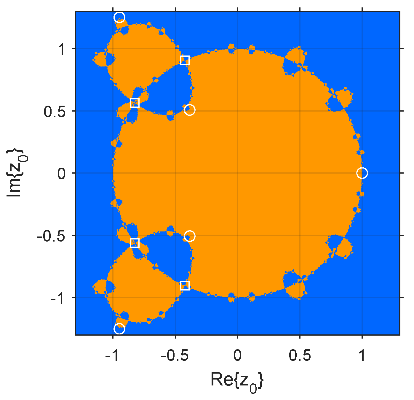
Dynamical planes illustrate the basins of attraction of the attracting fixed points, showing the stability of a single method. The implementation of the dynamical plane was developed in Matlab R2022b, following the guidelines of [30]. Figure 2 represents the dynamical plan of the rational operator . Orange and blue represent the basins of attraction of and , respectively. White circles refer to strange fixed points, while white squares represent free critical points. The dynamical plane only considers the initial guesses , since the rest of the dynamical plane is completely blue.
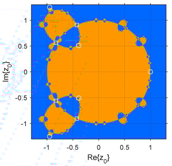
Figure 2.
Dynamical plane of .
The dynamical plane evidences the high stability of the iterative method for quadratic polynomials. Although the boundaries between the basins of attraction are intricate, each initial guess (except for the five extraneous fixed points) converges to a fixed attracting point that is coincident with the roots of the polynomial.
7. Numerical Results
This section elaborates on the utilization of numerical simulations for both scalar and vector forms of non-linear equations, integrating both theoretical and practical models. In the comparative analysis, we will examine specific parameters such as the number of iterations (i), the magnitude of absolute error ( for scalars and ( for vectors) at each iteration stage, and the processing time measured in CPU seconds. The simulations employed various iterative methodologies as delineated in Section 2, juxtaposed against the proposed fourth-order optimal iterative technique, as depicted in Equation (20) for scalars and (23) for systems. The numerical analyses in terms of tabular results were conducted using the software MAPLE 2022 on an Intel (R) Core (TM) i7 HP laptop equipped with 24 GB of RAM and operating at a frequency of 1.3 GHz while Python was used for graphical outputs. Regarding the numerical simulations, a maximum precision threshold of 4000 digits was established. Additionally, a cap of 50 iterations has been imposed to attain the requisite solution. The simulations are stopped based on the following halting criteria. For a single-variable nonlinear system (), we have the following:
and for a multi-variable nonlinear system, we have the following: ():
The following problems are considered from recent papers. The exact solution is shown against the test functions:
Problem 1.
.
Problem 2.
.
Problem 3
([31]). Boussinesq’s formula for vertical stress in the fields of soil mechanics and geotechnical engineering is given by the following:
Equation (57), when , can be written as follows:
In Table 1, the OPPNM method exhibits the most promising results when compared to OPNM1, OPNM2, OPNM3, and OPNM4. This method demonstrates rapid convergence toward the solution, particularly noticeable in the initial iterations across multiple problems and initial guesses, indicating a superior efficiency in approaching the correct solution quickly. While other methods show varying degrees of convergence and accuracy, OPPNM consistently reduces the absolute errors’ magnitude with each iteration, suggesting a robust performance across different nonlinear equations. Although some methods may reach lower errors at the final iteration, the speed and reliability of OPPNM in achieving a significant error reduction early on make it a potentially preferable method, especially in applications where a quick approximation is valuable. This aligns with the expectation that a proposed method should outperform existing ones, and in this context, the proposed optimal method OPPNM given in (20) fulfills the criteria effectively.

Table 1.
Numerical simulations for the scalar type of nonlinear equations presented in Problems 1–3.
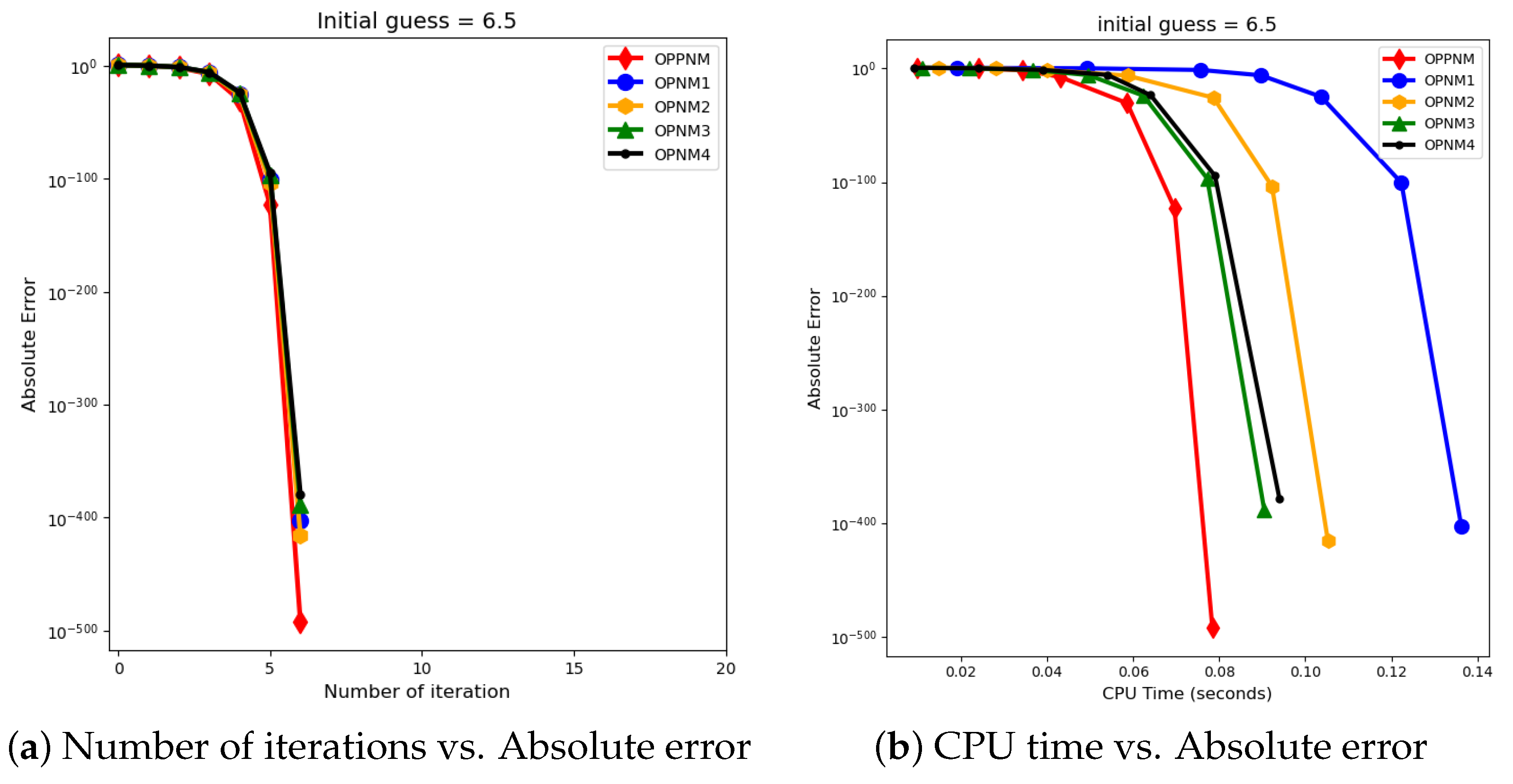
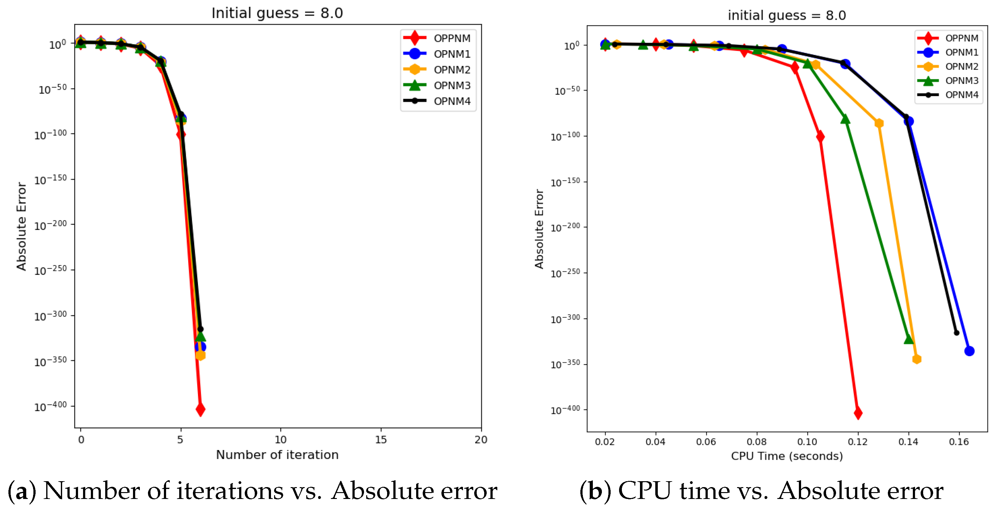
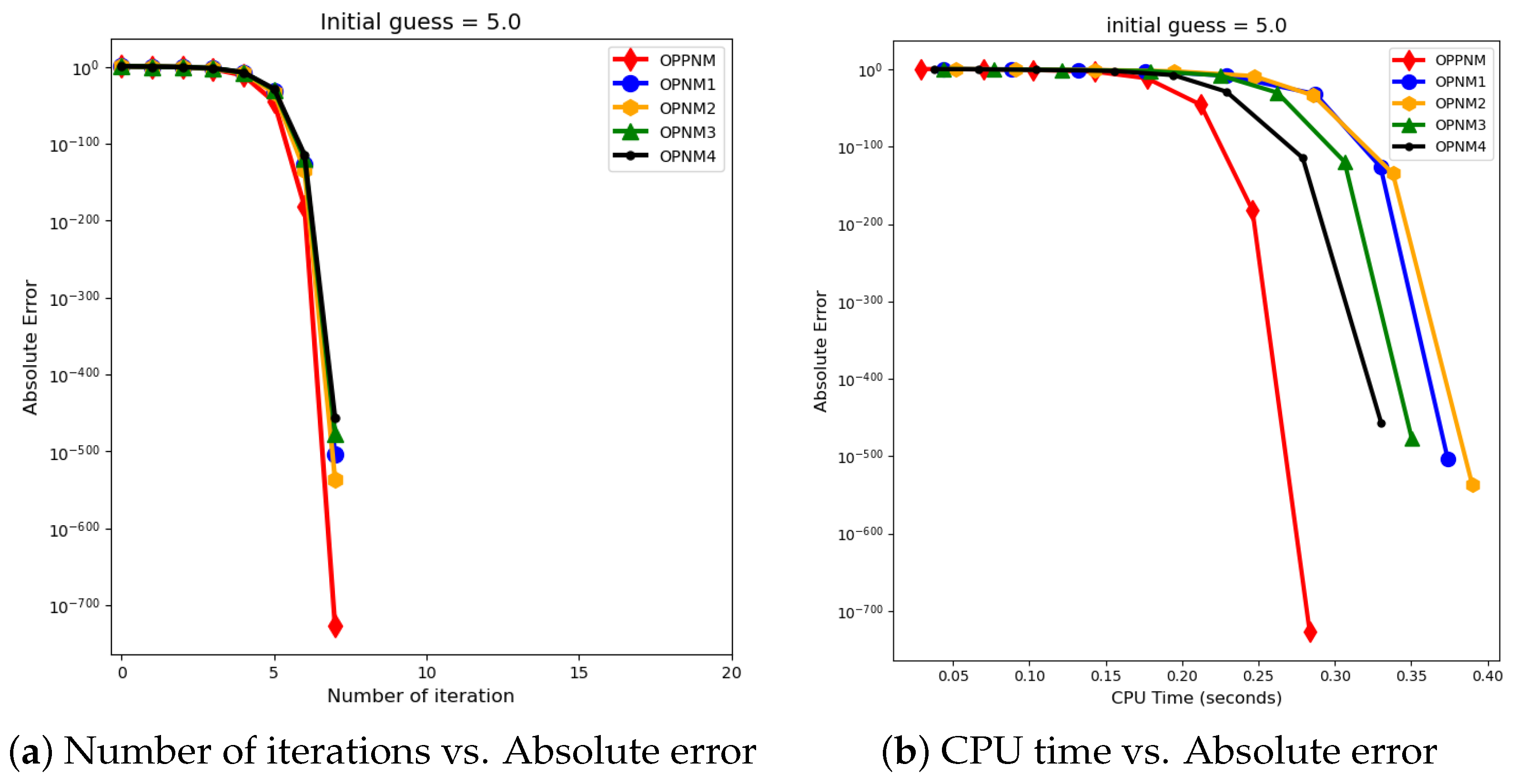
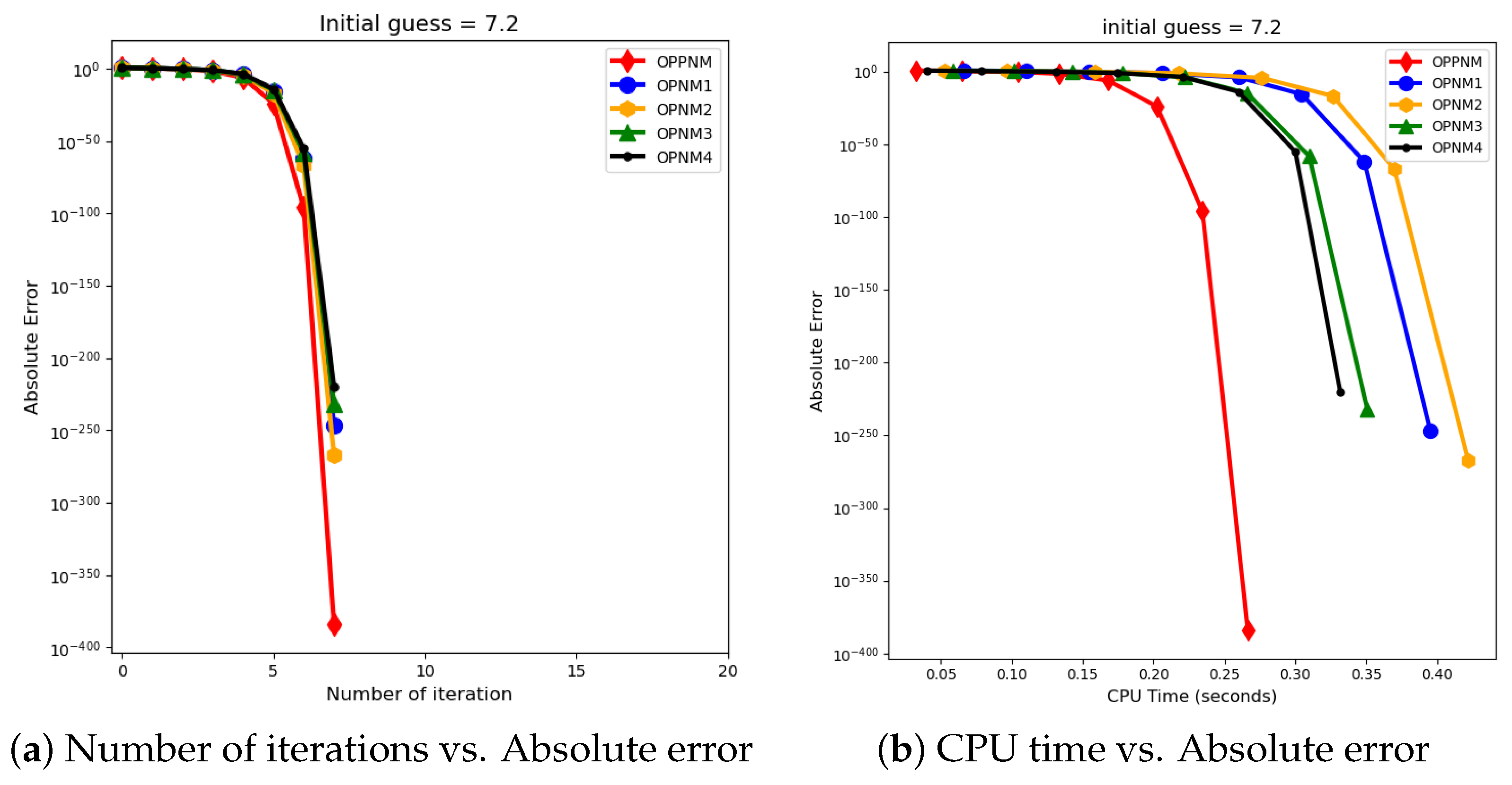
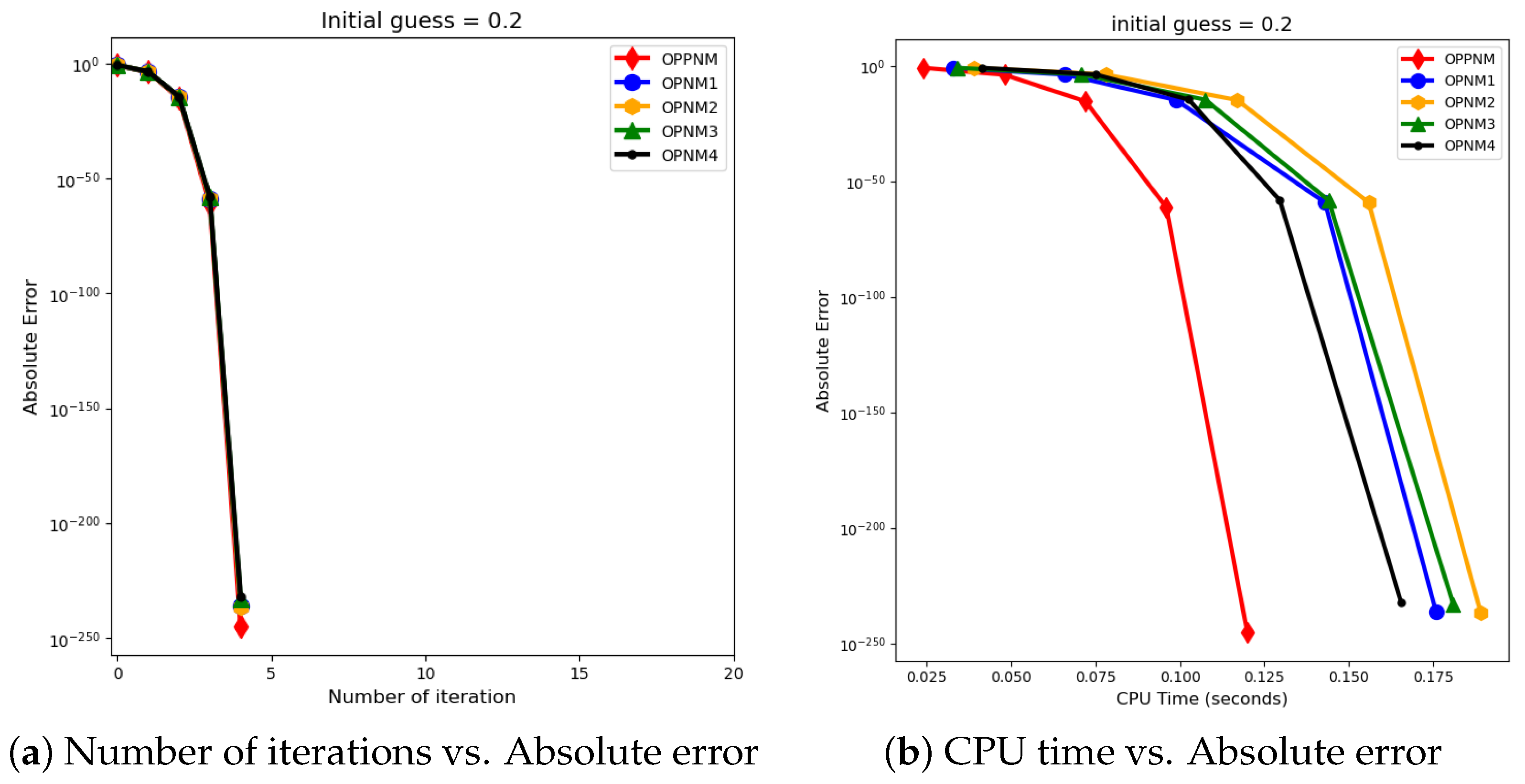
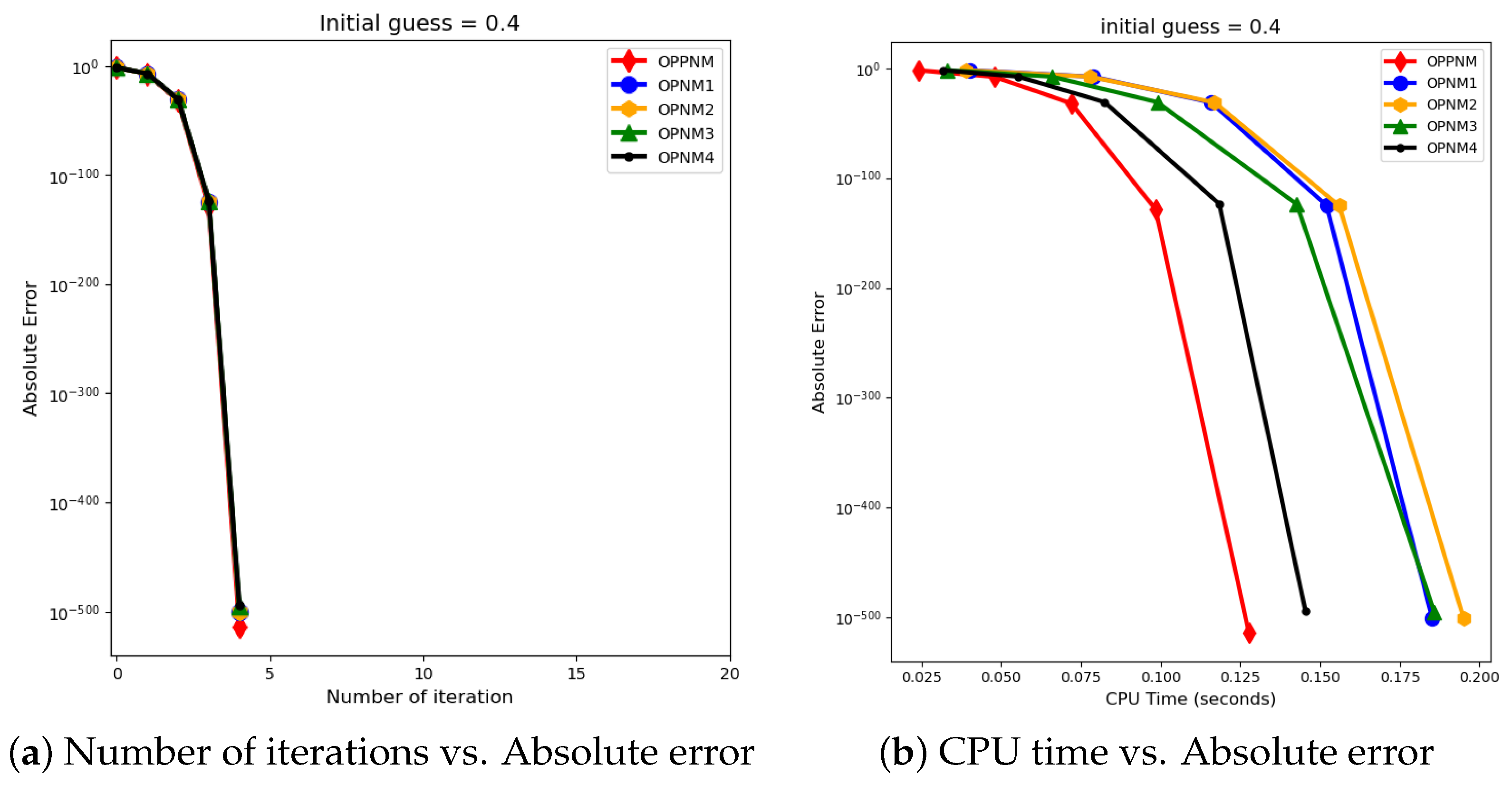
The graphical representation in the images illustrates a comparative study of different numerical solvers applied to the functions given in Problems 1–3. The efficiency curves are plotted in Figure 3, Figure 4, Figure 5, Figure 6, Figure 7 and Figure 8 to show the relationship between the precision of the solution, measured by the absolute error on the y-axis, and the computational effort, represented by the number of iterations and CPU time on the x-axis. In both sets of comparisons, the OPPNM method emerges as the most efficient. Specifically, for the initial guesses of 6.5 and 8.0 for , OPPNM achieves a rapid convergence to a low absolute error, outpacing the other methods. The steep descent of the OPPNM curves demonstrates its swift reduction in error as iterations progress, and it also shows significantly less CPU time required to reach a similar level of accuracy compared to its counterparts. This suggests a high rate of convergence and lower computational cost, making OPPNM the preferred solver based on the data presented. The claim that OPPNM is an optimal fourth-order method is substantiated by its apparent superior performance, both in terms of speed and computational resources. A similar sort of observation is made for Problems 2 and 3 in their efficiency curves.
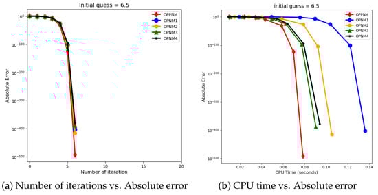
Figure 3.
Efficiency curves for the function with numerical solvers under consideration for .
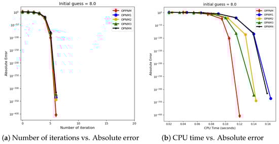
Figure 4.
Efficiency curves for the function with numerical solvers under consideration for .
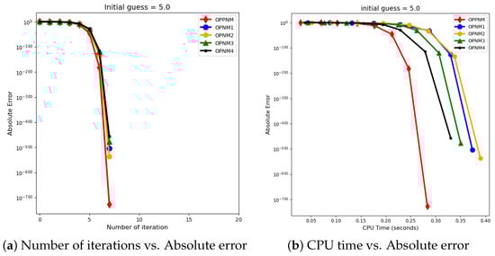
Figure 5.
Efficiency curves for the function with numerical solvers under consideration for .
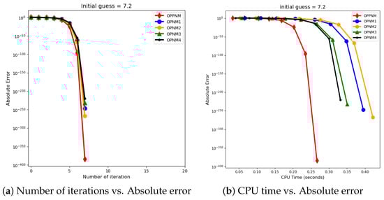
Figure 6.
Efficiency curves for the function with numerical solvers under consideration for .

Figure 7.
Efficiency curves for the function with numerical solvers under consideration for .
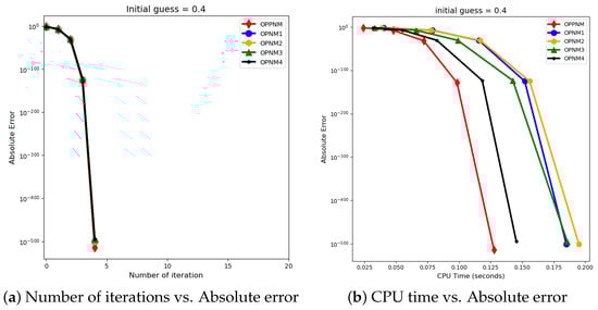
Figure 8.
Efficiency curves for the function with numerical solvers under consideration for .
The proposed fourth-order method (20) showcases notable progress in solving nonlinear equations of the form , establishing a fresh standard in computational efficiency. This methodology accelerates the calculation process and minimizes operating expenses by reaching the solution in fewer iterations and requiring the least CPU time compared to other optimal fourth-order algorithms as shown in Figure 3, Figure 4, Figure 5, Figure 6, Figure 7 and Figure 8. This efficiency is especially useful in large computing jobs and intricate simulations where time and resource allocation are critical. The method’s innovative algorithmic framework and exceptional performance make it the preferred choice for researchers and professionals seeking swift, precise, and cost-efficient solutions in applied mathematics, engineering, and other fields.
Given below are some nonlinear systems taken in higher dimensions. Table 2 compares the absolute errors of five numerical methods—labeled from OPPNM to OPNM4—applied to solve nonlinear systems of equations for Problems 4 through 8. The iterations are stopped when the desired accuracy mentioned in (56) is achieved. The OPPNM method, described as a “fourth-order optimal root-solver”, exhibits the lowest absolute errors across all iterations, indicating its superior accuracy and convergence rate. For instance, in Problem 4, the absolute error achieved by OPPNM is in the range of to , significantly outperforming the other methods. This trend of minimal errors is consistent across the problems listed, highlighting the effectiveness of the OPPNM method. The higher order of convergence inherent to OPPNM likely contributes to its ability to rapidly decrease errors with each iteration. This characteristic is crucial for achieving accurate solutions efficiently. Thus, the table substantiates the claim that OPPNM is the superior method among those compared, due to its optimal convergence properties and the consistently lower absolute errors it achieves, which aligns with expectations for a method touted as a fourth-order optimal root-solver. Moreover, in Problem 8, the focus is on the absolute errors of the last 7 iterations out of 24 for the OPPNM to OPNM4 methods. Here, the OPPNM method stands out with its absolute error reduction, showcasing errors diminishing from to an impressively low . This sharp decline in error magnitude demonstrates the method’s robustness and its capacity for high-precision solutions. In contrast, the other methods, OPNM1 through OPNM4, exhibit higher errors in the last iterations, with the smallest error being in the range of , which is significantly higher than that of OPPNM. This indicates that while the other methods are converging, they do so at a slower rate and with less accuracy. The OPPNM’s superior performance in the tail end of the iterations suggests stable convergence without signs of stagnation, underscoring its efficiency and effectiveness as a fourth-order optimal root-solver, particularly as the solution is refined in the final iterations.
Table 2.
Numerical simulations for the systems of nonlinear equations presented in Problems 4–8.
Problem 4.
The non-linear system of two equations from [14] is given as follows:
The initial guess is taken to be , where the exact solution of the system (59) is .
Problem 5.
The non-linear system of two equations from [14] is given as follows:
The initial guess is taken to be , where the exact solution of the system (60) is .
Problem 6.
The non-linear system of four equations from [14] is given as follows:
The initial guess is taken to be , where the exact solution of the system (61) is .
Problem 7.
Neurophysiology application [32,33]: The nonlinear model consists of the following six equations:
where the constants, , in the above model can be randomly chosen. In our experiment, we consider The initial guess is taken to be where the solution of the above system to the first few digits is as follows:
Problem 8.
Lastly, we consider a 10-dimensional nonlinear system that is related to combustion. The investigation of combustion phenomena at elevated temperatures, specifically at 3000 °C, formulated through a system of ten nonlinear algebraic equations by A. P. Morgan [34], serves as a quintessential exemplar of the intricate confluence of disciplines, including chemical engineering, thermodynamics, and applied numerical analysis.
The initial guess is taken to be , where the solution of the above system to the first few digits is as follows:
8. Conclusions and Future Remarks
This research highlights the important role played by nonlinear equations in various scientific fields, such as engineering, physics, and mathematics. Given the prevalence of mathematical models lacking closed solutions in these areas, the need for numerical methodologies, in particular root-solving algorithms, becomes evident. This study presents a new fourth-order convergent root solver that advances iterative approaches and offers improved accuracy. This solver—adapted to satisfy the optimality condition posed by the Kung–Traub conjecture by a linear combination—achieves an efficiency index of . By means of localized and semi-localized analyses, we rigorously discuss its convergence and efficiency. Furthermore, the examination of local and semi-local convergence, together with dynamic stability analysis, highlights the robustness of the solver in dealing with systems of nonlinear equations. Empirical validations using mathematical models from various fields such as physics, mechanics, chemistry, and combustion have demonstrated the superior performance of the proposed solver.
For future research, it would be beneficial to explore the integration of this solver with machine learning algorithms to further improve its predictive capabilities and its effectiveness in solving even more complex systems of equations. This could open new avenues for solving real-world problems with unprecedented accuracy and speed.
Author Contributions
Conceptualization, S.Q. and I.K.A.; methodology, S.Q. and E.H.; software, F.I.C. and A.S.; validation, J.A. and E.H.; formal analysis, S.Q. and I.K.A.; investigation, S.Q.; resources, J.A.; writing—original draft preparation, A.S.; writing—review and editing, F.I.C.; visualization, J.A.; supervision, S.Q.; project administration, S.Q.; funding acquisition, F.I.C. All authors have read and agreed to the published version of the manuscript.
Funding
F.I.C. received partial funding from “Ayuda a Primeros Proyectos de Investigación (PAID-06-23), Vicerrectorado de Investigación de la Universitat Politècnica de València (UPV)”, in the project MERLIN framework.
Data Availability Statement
Data are contained within the article.
Acknowledgments
The authors are especially grateful to the reviewers, whose reports have significantly improved the final version of this article.
Conflicts of Interest
The authors declare no conflicts of interest. The funders had no role in the design of the study; in the collection, analyses, or interpretation of data; in the writing of the manuscript; or in the decision to publish the results.
References
- Faires, J.; Burden, R. Numerical Methods, 4th ed.; Cengage Learning: Belmont, CA, USA, 2012. [Google Scholar]
- Naseem, A.; Rehman, M.; Abdeljawad, T. A novel root-finding algorithm with engineering applications and its dynamics via computer technology. IEEE Access 2022, 10, 19677–19684. [Google Scholar] [CrossRef]
- Abro, H.A.; Shaikh, M.M. A new family of twentieth order convergent methods with applications to nonlinear systems in engineering. Mehran Univ. Res. J. Eng. Technol. 2023, 42, 165–176. [Google Scholar] [CrossRef]
- Shaikh, M.M.; Massan, S.-u.-R.; Wagan, A.I. A sixteen decimal places’ accurate Darcy friction factor database using non-linear Colebrook’s equation with a million nodes: A way forward to the soft computing techniques. Data Brief 2019, 27, 104733. [Google Scholar] [CrossRef]
- Argyros, M.I.; Argyros, I.K.; Regmi, S.; George, S. Generalized three-step numerical methods for solving equations in banach spaces. Mathematics 2022, 10, 2621. [Google Scholar] [CrossRef]
- Ramos, H.; Monteiro, M.T.T. A new approach based on the Newton’s method to solve systems of nonlinear equations. J. Comput. Appl. Math. 2017, 318, 3–13. [Google Scholar] [CrossRef]
- Ramos, H.; Vigo-Aguiar, J. The application of Newton’s method in vector form for solving nonlinear scalar equations where the classical Newton method fails. J. Comput. Appl. Math. 2015, 275, 228–237. [Google Scholar] [CrossRef]
- Abdullah, S.; Choubey, N.; Dara, S. Optimal fourth-and eighth-order iterative methods for solving nonlinear equations with basins of attraction. J. Appl. Math. Comput. 2024. [Google Scholar] [CrossRef]
- Yun, J.H. A note on three-step iterative method for nonlinear equations. Appl. Math. Comput. 2008, 202, 401–405. [Google Scholar] [CrossRef]
- Dehghan, M.; Shirilord, A. Three-step iterative methods for numerical solution of systems of nonlinear equations. Eng. Comput. 2022, 38, 1015–1028. [Google Scholar] [CrossRef]
- Soleymani, F.; Vanani, S.K.; Afghani, A. A general three-step class of optimal iterations for nonlinear equations. Math. Prob. Eng. 2011, 2011, 469512. [Google Scholar] [CrossRef]
- Darvishi, M. Some three-step iterative methods free from second order derivative for finding solutions of systems of nonlinear equations. Int. J. Pure Appl. Math. 2009, 57, 557–573. [Google Scholar]
- Kung, H.; Traub, J.F. Optimal order of one-point and multipoint iteration. J. ACM 1974, 21, 643–651. [Google Scholar] [CrossRef]
- Singh, A.; Jaiswal, J. Several new third-order and fourth-order iterative methods for solving nonlinear equations. Int. J. Eng. Math. 2014, 2014, 828409. [Google Scholar] [CrossRef]
- Jaiswal, J.P. Some class of third-and fourth-order iterative methods for solving nonlinear equations. J. Appl. Math. 2014, 2014, 817656. [Google Scholar] [CrossRef]
- Sharma, E.; Panday, S.; Dwivedi, M. New optimal fourth order iterative method for solving nonlinear equations. Int. J. Emerg. Technol. 2020, 11, 755–758. [Google Scholar]
- Khattri, S.K.; Abbasbandy, S. Optimal fourth order family of iterative methods. Matematički Vesnik 2011, 63, 67–72. [Google Scholar]
- Chun, C.; Lee, M.Y.; Neta, B.; Džunić, J. On optimal fourth-order iterative methods free from second derivative and their dynamics. Appl. Math. Comput. 2012, 218, 6427–6438. [Google Scholar] [CrossRef]
- Panday, S.; Sharma, A.; Thangkhenpau, G. Optimal fourth and eighth-order iterative methods for non-linear equations. J. Appl. Math. Comput. 2023, 69, 953–971. [Google Scholar] [CrossRef]
- Abro, H.A.; Shaikh, M.M. A new time-efficient and convergent nonlinear solver. Appl. Math. Comput. 2019, 355, 516–536. [Google Scholar] [CrossRef]
- Qureshi, S.; Ramos, H.; Soomro, A.K. A New Nonlinear Ninth-Order Root-Finding Method with Error Analysis and Basins of Attraction. Mathematics 2021, 9, 1996. [Google Scholar] [CrossRef]
- Argyros, I. Unified Convergence Criteria for Iterative Banach Space Valued Methods with Applications. Mathematics 2021, 9, 1942. [Google Scholar] [CrossRef]
- Argyros, I. The Theory and Applications of Iteration Methods, 2nd ed.; CRC Press: Boca Raton, FL, USA, 2022. [Google Scholar] [CrossRef]
- Devaney, R.L. An Introduction to Chaotic Dynamical Systems; Addison-Wesley: Boston, MA, USA, 1989. [Google Scholar]
- Beardon, A.F. Iteration of Rational Functions: Complex Analytic Dynamical Systems; Springer: New York, NY, USA, 1991. [Google Scholar]
- Wang, X.; Chen, X.; Li, W. Dynamical behavior analysis of an eighth-order Sharma’s method. Intl. J. Biomath. 2023, 2023, 2350068. [Google Scholar] [CrossRef]
- Kroszczynski, K.; Kiliszek, D.; Winnicki, I. Some Properties of the Basins of Attraction of the Newton’s Method for Simple Nonlinear Geodetic Systems. Preprints 2021, 2021120151. [Google Scholar] [CrossRef]
- Campos, B.; Villalba, E.G.; Vindel, P. Dynamical and numerical analysis of classical multiple roots finding methods applied for different multiplicities. Comput. Appl. Math. 2024, 43, 230. [Google Scholar] [CrossRef]
- Campos, B.; Canela, J.; Vindel, P. Dynamics of Newton-line root finding methods. Numer. Algorithms 2023, 93, 1453–1480. [Google Scholar] [CrossRef]
- Chicharro, F.I.; Cordero, A.; Torregrosa, J.R. Drawing Dynamical and Parameters Planes of Iterative Families and Methods. Sci. World J. 2013, 2013, 708153. [Google Scholar] [CrossRef]
- Abdullah, S.; Choubey, N.; Dara, S. An efficient two-point iterative method with memory for solving non-linear equations and its dynamics. J. Appl. Math. Comput. 2024, 70, 285–315. [Google Scholar] [CrossRef]
- Verschelde, J.; Verlinden, P.; Cools, R. Homotopies exploiting Newton polytopes for solving sparse polynomial systems. SIAM J. Numer. Anal. 1994, 31, 915–930. [Google Scholar] [CrossRef]
- Grosan, C.; Abraham, A. A new approach for solving nonlinear equations systems. IEEE Trans. Syst. Man Cybern.-Part A Syst. Hum. 2008, 38, 698–714. [Google Scholar] [CrossRef]
- Morgan, A. Solving Polynomial Systems Using Continuation for Engineering and Scientific Problems; SIAM: Philadelphia, PA, USA, 2009. [Google Scholar]
Disclaimer/Publisher’s Note: The statements, opinions and data contained in all publications are solely those of the individual author(s) and contributor(s) and not of MDPI and/or the editor(s). MDPI and/or the editor(s) disclaim responsibility for any injury to people or property resulting from any ideas, methods, instructions or products referred to in the content. |
© 2024 by the authors. Licensee MDPI, Basel, Switzerland. This article is an open access article distributed under the terms and conditions of the Creative Commons Attribution (CC BY) license (https://creativecommons.org/licenses/by/4.0/).