Randomly Stopped Sums, Minima and Maxima for Heavy-Tailed and Light-Tailed Distributions

Abstract

This paper investigates the randomly stopped sums, minima and maxima of heavy- and light-tailed random variables. The conditions on the primary random variables, which are independent but generally not identically distributed, and counting random variable are given in order that the randomly stopped sum, random minimum and maximum is heavy/light tailed. The results generalize some existing ones in the literature. The examples illustrating the results are provided.

1. Introduction

This paper is devoted to the randomly stopped sums, minima and maxima of heavy- and light-tailed random variables (r.v.s). Such objects appear when the number of the random variables under consideration is unknown and is described by some random integer. In particular, randomly stopped sums appear in such fields as insurance and financial mathematics, survival analysis, risk theory, computer and communication networks, etc. The area of randomly stopped sums for heavy-tailed r.v.s has been well developed for more than 50 years and covers mainly the case of independent identically distributed (i.i.d.) r.v.s. In this paper, we consider the case where the underlying r.v.s are not necessarily identically distributed, although they are independent.

Specifically, suppose that $X_1,X_2,\cdots$ are r.v.s defined on the probability space $(\mathrm{\Omega },\mathcal{F},\mathbb{P})$. Define a sequence of partial sums $\{S_n,n\ge 0\}$ by

$$\begin{array}{c}\hfill S_0:=0,S_n:=X_1+\cdots +X_n,n\ge 1.\end{array}$$

(1)

The main subject of the paper lies in the study of randomly stopped sums:

$$\begin{array}{c}\hfill S_{\nu }:=X_1+\cdots +X_{\nu },\end{array}$$

where n in (1) is replaced by a random variable $\nu$, taking values in ${\mathbb{N}}_0:=\{0,1,2,\cdots \}$. Throughout this paper, we assume that $\nu$ is not degenerate at zero, i.e., $\mathbb{P}(\nu >0)>0$. We will call such $\nu$ a counting random variable.

Further, we will assume that r.v.s $X_1,X_2,\cdots$ are independent and counting r.v. $\nu$ is independent of the sequence $\{X_1,X_2,\cdots \}$. In general, r.v.s $X_1,X_2,\cdots$ can be not identically distributed, each having a distribution function (d.f.) $F_{X_k}\left(x\right)=\mathbb{P}(X_k\le x)$, respectively. Consider the d.f.

$$\begin{array}{cc}\hfill F_{S_{\nu }}\left(x\right)& =\mathbb{P}(S_{\nu }\le x)=\sum _{n=0}^{\infty }\mathbb{P}(S_n\le x)\mathbb{P}(\nu =n).\hfill \end{array}$$

The main task considered in this paper is to give conditions guaranteeing that $F_{S_{\nu }}$ is heavy-/light-tailed, provided that some of the d.f.s $F_{X_k}$ or $F_{\nu }$ are heavy-/light-tailed.

Other objects of the paper are the randomly stopped minima and maxima. By the randomly stopped minimum of sums, we call the minimum of partial sums:

$$\begin{array}{cc}\hfill S_{\left(\nu \right)}& =\left\{\begin{array}{cc}min\{S_1,\cdots ,S_{\nu }\},\hfill & \nu \ge 1,\hfill \\ 0,\hfill & \nu =0,\hfill \end{array}\right.\hfill \end{array}$$

and by the rrandomly stopped maximum of sums, we call the maximum of partial sums:

$$\begin{array}{c}\hfill S^{\left(\nu \right)}=max\{0,S_1,\cdots ,S_{\nu }\}.\end{array}$$

Also, we provide some results for the randomly stopped minimum,

$$\begin{array}{cc}\hfill X_{\left(\nu \right)}& =\left\{\begin{array}{cc}min\{X_1,\cdots ,X_{\nu }\},\hfill & \nu \ge 1,\hfill \\ 0,\hfill & \nu =0,\hfill \end{array}\right.\hfill \end{array}$$

and the randomly stopped maximum,

$$\begin{array}{c}\hfill X^{\left(\nu \right)}=max\{0,X_1,\cdots ,X_{\nu }\}.\end{array}$$

Similarly, we are interested in when $F_{X_{\left(\nu \right)}}$, $F_{X^{\left(\nu \right)}}$, $F_{S_{\left(\nu \right)}}$ and $F_{S^{\left(\nu \right)}}$ are heavy-tailed or light-tailed. The most attention we pay is to the closure of heavy-tailed and light-tailed classes of distributions with respect to random transformations under consideration. For example, Proposition 1 (see parts (iii), (iv)) below implies that a randomly stopped sum remains heavy-tailed if at least one of the primary r.v.s $\{X_1,X_2,\dots \}$ reached by the counting r.v. $\nu$ is heavy-tailed. Proposition 2 (see parts (i), (ii)) shows that the randomly stopped maximum has an analogous property. Meanwhile, Proposition 3 (i) shows that the randomly stopped minimum remains heavy-tailed if the first primary r.v. $X_1$ is heavy-tailed, and the tails of other primary r.v.s are asymptotically compared to the distribution tail of the first primary r.v. Proposition 5 (iii) implies that the randomly stopped maximum of sums for any counting r.v. remains heavy-tailed if the first primary r.v. $X_1$ is heavy tailed. Meanwhile, according to Proposition 4 (i), in order for the randomly stopped maximum to remain heavy-tailed, it is necessary that the other primary r.v.s $\{X_2,X_3,\dots \}$ obtain some nonnegative values. Similar facts about the closure of the class of light-tailed distributions with respect to the considered transformations can also be obtained from Propositions 1–5 below. For various distribution classes, similar questions on the closure with respect to various transformations have been studied in [1,2,3,4,5,6,7,8,9,10,11,12,13,14,15,16,17,18,19,20,21,22,23,24,25,26,27,28,29,30]. In particular, regularly varying distributions were considered in [23], consistently varying distributions in [2,15], long-tailed distributions in [18,19,21] and dominatedly varying distributions in [6,18,19]. Maxima and sums of nonstationary random-length sequences of random variables with regularly varying tails were studied in [31]. We mention also paper [32], where two independent heavy-tailed r.v.s, such that their minimum is not heavy tailed, were constructed.

One of the incentives to study the randomly stopped structures is related to the models describing the insurance business. According to the well-known Sparre Andersen model [33], the insurer’s wealth $W_u\left(t\right)$ is described by the risk renewal model:

$$W_u\left(t\right)=u+pt-\sum _{k=1}^{N_{\theta }\left(t\right)}{Z}_k,t\ge 0,$$

where $u\ge 0$ is the initial capital, $p>0$ is a constant premium rate, $N_{\theta }\left(t\right)$ is a counting process generated by a sequence of not negative r.v.s $\{{\theta }_1,{\theta }_2,\dots \}$ and $\{Z_1,Z_2,\dots \}$ is a sequence of independent random claims. Due to such a model, the behavior of the insurer’s wealth $W_u\left(t\right)$ is driven by the randomly stopped sums

$$S_{\theta }\left(t\right)=\sum _{k=1}^{N_{\theta }\left(t\right)}{Z}_k,t\ge 0,$$

and the model ruin probability,

$$\psi \left(u\right)=\mathbb{P}\left(\underset{t>0}{inf}{W}_u\left(t\right)<0\right)$$

is related to maximum of the randomly stopped sums

$$\underset{0<t\le T}{max}{S}_{\theta }\left(t\right).$$

It is well known that the behavior of $S_{\theta }\left(t\right)$, the selection of the premium rate p and the estimation of the ruin probability depends on whether the generating elements $\{{\theta }_1,{\theta }_2,\dots \}$, $\{Z_1,Z_2,\dots \}$ and $S_{\theta }\left(t\right)$ have light tails or heavy tails, even in the case that the distributions generating the model are identically distributed. For details, see [34,35,36,37,38].

We also note the well known duality of the homogeneous risk renewal model and the G/G/1 model from queuing theory, where the arrivals follow the counting process generated by distribution $F_{\theta }$ and service times have distribution $F_Z$. Then the probability of ruin $\psi \left(u\right)$ coincides with the probability that the stationary waiting time exceeds u. For details see [34].

The structure of the paper is as follows. In Section 2, we introduce heavy- and light-tailed distributions and formulate two auxiliary lemmas. The main results are formulated in Section 3. Some examples of nonstandard heavy-tailed and light-tailed distributions are presented in Section 4. The heaviness of the distribution tails presented in Section 4 is determined on the basis of the statements formulated in Section 3. The proofs of the main results are presented in Section 5. The last Section 6 is devoted to the discussion of the obtained results in the broadest context together with the highlighting of future research directions.

2. Heavy-Tailed and Light-Tailed Distributions

For any distribution F, define its Laplace–Stieltjes transform as

$$\begin{array}{c}\hfill \widehat{F}\left(\lambda \right):={\int }_{-\infty }^{\infty }{\mathrm{e}}^{\lambda x}\mathrm{d}F\left(x\right),\lambda \in \mathbb{R}.\end{array}$$

A distribution F is said to be heavy-tailed, denoted $F\in \mathcal{H}$, if

$$\begin{array}{c}\hfill \widehat{F}\left(\lambda \right)=\infty \mathrm{for}\mathrm{any}\lambda >0.\end{array}$$

Otherwise, F is said to be light-tailed. Common examples of heavy-tailed distributions are Pareto, log-normal, Weibull with shape parameter $\tau \in (0,1)$, Burr and Student’s t distributions. For a detailed exposition of the heavy-tailed distributions and their properties, we refer to monographs [36,39,40,41,42,43,44].

We formulate two lemmas that will be used in the proofs of several main propositions. Although the results of the lemmas are well known and can be found, e.g., in [41,43,44], we provide the proofs for the sake of convenience. The first lemma gives equivalent conditions for the distribution F to be heavy-/light-tailed.

Lemma 1. 

Suppose that F is a d.f. of a real-valued r.v. The following statements are equivalent:

(i)

F is heavy-tailed,

(ii)

$\underset{x\to \infty }{lim\; sup}{\mathrm{e}}^{\lambda x}\overline{F}\left(x\right)=\infty$ for any $\lambda >0$,

(iii)

$\underset{x\to \infty }{lim\; sup}{x}^{-1}log\overline{F}\left(x\right)=0$.

Similarly, the equivalent are the following statements:

(i’)

F is light-tailed,

(ii’)

$\underset{x\to \infty }{lim\; sup}{\mathrm{e}}^{\lambda x}\overline{F}\left(x\right)<\infty$ for some $\lambda >0$,

(iii’)

$\underset{x\to \infty }{lim\; sup}{x}^{-1}log\overline{F}\left(x\right)<0$.

Proof. 

We prove only the first part of the lemma.

(i) ⇒ (iii). Suppose that $\widehat{F}\left(\lambda \right)=\infty$ for any $\lambda >0$. Let, on the contrary,

$$\begin{array}{c}\hfill \underset{x\to \infty }{lim\; sup}\frac{log\overline{F}\left(x\right)}{x}<0.\end{array}$$

Then, there exist constants $c>0$ and $x_c>0$ such that $x^{-1}log\overline{F}\left(x\right)\le -c$ for $x\ge x_c$, or, equivalently,

$$\begin{array}{c}\hfill \overline{F}\left(x\right)\le {\mathrm{e}}^{-cx},x\ge x_c.\end{array}$$

(2)

For any $\delta \in (0,c)$, using (2) and the alternative expectation formula (see [45], for instance), we obtain

$$\begin{array}{cc}\hfill {\int }_{[0,\infty )}{\mathrm{e}}^{\delta u}\mathrm{d}F\left(u\right)& =1+\delta {\int }_0^{\infty }{\mathrm{e}}^{\delta u}\overline{F}\left(u\right)\mathrm{d}u\hfill \\ & =1+\left({\int }_1^{{\mathrm{e}}^{\delta x_c}}+{\int }_{{\mathrm{e}}^{\delta x_c}}^{\infty }\right)\overline{F}\left({\delta }^{-1}logu\right)\mathrm{d}u\hfill \\ \hfill & \le {\mathrm{e}}^{\delta x_c}+{\int }_{{\mathrm{e}}^{\delta x_c}}^{\infty }{\mathrm{e}}^{-c{\delta }^{-1}logu}\mathrm{d}u\hfill \\ \hfill & ={\mathrm{e}}^{\delta x_c}+{\int }_{{\mathrm{e}}^{\delta x_c}}^{\infty }{u}^{-c{\delta }^{-1}}\mathrm{d}u.\hfill \end{array}$$

Since $c{\delta }^{-1}>1$, the last integral is finite; hence,

$$\begin{array}{c}\hfill \widehat{F}\left(\delta \right)\le F\left(0\right)+{\int }_{[0,\infty )}{\mathrm{e}}^{\delta u}\mathrm{d}F\left(u\right)<\infty ,\end{array}$$

leading to a contradiction.

(iii) ⇒ (ii). From the condition

$$\underset{x\to \infty }{lim\; sup}{x}^{-1}log\overline{F}\left(x\right)=0$$

we obtain that there exists an infinitely increasing sequence $\left\{x_n\right\}$ such that

$$\underset{n\to \infty }{lim}{x}_n^{-1}log\overline{F}\left(x_n\right)=0.$$

For any given $\lambda >0$, this implies that there exists $n_{\lambda }\ge 1$ such that

$$x_n^{-1}log\overline{F}\left(x_n\right)\ge -\lambda /2$$

for all $n\ge n_{\lambda }$. Equivalently,

$$\begin{array}{c}\hfill {\mathrm{e}}^{\lambda x_n}\overline{F}\left(x_n\right)\ge {\mathrm{e}}^{\lambda x_n/2},n\ge n_{\lambda }.\end{array}$$

Hence, ${\mathrm{e}}^{\lambda x_n}\overline{F}\left(x_n\right)$ tends to infinity as $n\to \infty$, and thus,

$$\begin{array}{c}\hfill \underset{x\to \infty }{lim\; sup}{\mathrm{e}}^{\lambda x}\overline{F}\left(x\right)\ge \underset{n\to \infty }{lim}{\mathrm{e}}^{\lambda x_n}\overline{F}\left(x_n\right)=\infty .\end{array}$$

Since this holds for any $\lambda >0$, we have (ii).

(ii) ⇒ (i). Let

$$\underset{x\to \infty }{lim\; sup}{\mathrm{e}}^{\lambda x}\overline{F}\left(x\right)=\infty$$

for any $\lambda >0$. For $x\in \mathbb{R}$, write

$$\begin{array}{c}\hfill {\int }_{-\infty }^{\infty }{\mathrm{e}}^{\lambda u}\mathrm{d}F\left(u\right)\ge {\int }_{(x,\infty )}{\mathrm{e}}^{\lambda u}\mathrm{d}F\left(u\right)\ge {\mathrm{e}}^{\lambda x}\overline{F}\left(x\right).\end{array}$$

Thus,

$$\begin{array}{c}\hfill \widehat{F}\left(\lambda \right)\ge \underset{x\to \infty }{lim\; sup}{\mathrm{e}}^{\lambda x}\overline{F}\left(x\right)=\infty \mathrm{for}\mathrm{any}\lambda >0,\end{array}$$

and Lemma 1 is proved. □

The next lemma implies that $\mathcal{H}$ and ${\mathcal{H}}^c$ are closed with respect to weak tail equivalence.

Lemma 2. 

Let F and G be two distributions of real-valued r.v.s.

(i)

If $F\in \mathcal{H}$ and

$$\underset{x\to \infty }{lim\; inf}\frac{\overline{G}\left(x\right)}{\overline{F}\left(x\right)}>0,$$

(3)

then $G\in \mathcal{H}$.

(ii)

If $F\in {\mathcal{H}}^c$, and $\overline{G}\left(x\right)\le \tilde{c}\overline{F}\left(x\right)$ for some $\tilde{c}>0$ and large x ($x>x_{\tilde{c}}$), then $G\in {\mathcal{H}}^c$.

Proof. 

Consider part (i). By condition (3), we obtain that

$$\overline{G}\left(x\right)\ge \widehat{c}\overline{F}\left(x\right)$$

for some $\widehat{c}$ and sufficiently large x ($x>x_{\widehat{c}}$). Therefore,

$$\begin{array}{c}\hfill \underset{x\to \infty }{lim\; sup}{\mathrm{e}}^{\lambda x}\overline{G}\left(x\right)\ge \widehat{c}\underset{x\to \infty }{lim\; sup}{\mathrm{e}}^{\lambda x}\overline{F}\left(x\right)=\infty \end{array}$$

for any positive $\lambda$ implying $G\in \mathcal{H}$ by Lemma 1 (ii).

The proof of part (ii) can be constructed in a similar way by using Lemma 1 (ii’), showing that

$$\begin{array}{c}\hfill \underset{x\to \infty }{lim\; sup}{\mathrm{e}}^{\lambda x}\overline{G}\left(x\right)<\infty \end{array}$$

for some $\lambda >0$. Lemma 2 is proved. □

3. Main Results

In this section, we formulate the main results of the paper. We start with the randomly stopped sums. We notice that the d.f. $F_{S_{\nu }}$ can become heavy-tailed because of the heavy tail of some element in $\{F_{X_1},F_{X_2},\dots \}$ or because of the heavy tail of the counting random variable $\nu$.

Proposition 1. 

Let $X_1,X_2,\dots$ be independent real-valued r.v.s and let ν be a counting r.v. independent of the sequence $\{X_1,X_2,\dots \}$. Distribution $F_{S_{\nu }}$ is heavy-tailed if at least one of the following conditions is satisfied:

(i)

$\underset{k\ge 1}{inf}\mathbb{E}{\mathrm{e}}^{\lambda X_k}>1$ for any $\lambda >0$, and $F_{\nu }\in \mathcal{H}$;

(ii)

$\underset{k\ge 1}{inf}\mathbb{P}(X_k\ge a)=1$ for some $a>0$, and $F_{\nu }\in \mathcal{H}$;

(iii)

$F_{X_{\varkappa }}\in \mathcal{H}$ for some $\varkappa \ge 1$, and $\overline{F_{\nu }}\left(x\right)>0$ for all $x\in \mathbb{R}$;

(iv)

$F_{X_{\varkappa }}\in \mathcal{H}$ for some $1\le \varkappa \le max\left\{\mathrm{supp}\right(\nu \left)\right\}$ and $\mathrm{supp}\left(\nu \right)<\infty$.

Distribution $F_{S_{\nu }}$ is light-tailed if at least one of the following conditions is satisfied:

(v)

$F_{X_1}\in {\mathcal{H}}^c$, $F_{\nu }\in {\mathcal{H}}^c$, $\overline{F_{X_1}}\left(x\right)>0$ for all $x\in \mathbb{R}$ and

$$\underset{x\to \infty }{lim\; sup}\underset{k\ge 1}{sup}\frac{\overline{F_{X_k}}\left(x\right)}{\overline{F_{X_1}}\left(x\right)}<\infty ;$$

(4)

(vi)

$\underset{k\ge 1}{sup}\mathbb{E}{\mathrm{e}}^{\lambda X_k}<\infty$ for some $\lambda >0$, and $F_{\nu }\in {\mathcal{H}}^c$.

Our next statement is about the randomly stopped maximum of r.v.s. We observe that some conditions under which the distribution of the randomly stopped maximum $F_{X^{\left(\nu \right)}}$ becomes heavy-tailed are the same as in Proposition 1. Unfortunately, we did not find how to make a heavy-tailed distribution $F_{X^{\left(\nu \right)}}$ from the light-tailed primary r.v.s $\{X_1,X_2,\dots \}$.

Proposition 2. 

Let $X_1,X_2,\dots$ be independent real-valued r.v.s and let ν be a counting r.v. independent of the sequence $\{X_1,X_2,\dots \}$.

(i)

If $F_{X_{\varkappa }}\in \mathcal{H}$ for some $\varkappa \ge 1$ and $\overline{F_{\nu }}\left(x\right)>0$ for all $x\in \mathbb{R}$, then $F_{X^{\left(\nu \right)}}\in \mathcal{H}$;

(ii)

If $F_{X_{\varkappa }}\in \mathcal{H}$ for some $\varkappa \le max\left\{\mathrm{supp}\right(\nu \left)\right\}<\infty$, then $F_{X^{\left(\nu \right)}}\in \mathcal{H}$;

(iii)

Distribution $F_{X^{\left(\nu \right)}}$ belongs to the class ${\mathcal{H}}^c$ if $F_{X_1}\in {\mathcal{H}}^c$, $\overline{F_{X_1}}\left(x\right)>0$ for all $x\in \mathbb{R}$, $\mathbb{E}\nu <\infty$ and

$$\begin{array}{cc}\hfill \underset{x\to \infty }{lim\; sup}\underset{n\ge 1}{sup}\frac{1}{n}\sum _{k=1}^n\frac{\overline{F_{X_k}}\left(x\right)}{\overline{F_{X_1}}\left(x\right)}& <\infty .\hfill \end{array}$$

(5)

The statement below is on the distribution of the randomly stopped minimum of r.v.s. From the formulation below, we observe that the tail of the d.f. $F_{X_{\left(\nu \right)}}$ has much less chance of becoming heavy compared to the d.f.s $F_{S_{\nu }}$ and $F_{X^{\left(\nu \right)}}$.

Proposition 3. 

Let $X_1,X_2,\dots$ be independent real-valued r.v.s and let ν be a counting r.v. independent of the sequence $\{X_1,X_2,\dots \}$.

(i)

If $F_{X_1}\in \mathcal{H}$ and

$$\underset{x\to \infty }{lim\; inf}\underset{1\le k\le \varkappa }{min}\frac{\overline{F_{X_k}}\left(x\right)}{\overline{F_{X_1}}\left(x\right)}>0$$

for $\varkappa =min\left\{\mathrm{supp}\right(\nu )\setminus \{0\left\}\right\}$, then $F_{X_{\left(\nu \right)}}\in \mathcal{H}$ and

$$\overline{F_{X_{\left(\nu \right)}}}\left(x\right)\underset{x\to \infty }{\sim }\mathbb{P}(\nu =\varkappa )\overline{F_{X_{\left(\varkappa \right)}}}\left(x\right);$$

(ii)

If $F_{X_k}\in {\mathcal{H}}^c$ for $1\le k\le \varkappa =min\left\{\mathrm{supp}\right(\nu )\setminus \{0\left\}\right\}$, then $F_{X_{\left(\nu \right)}}\in {\mathcal{H}}^c$.

The next two statements are on the heaviness of randomly stopped minimum of sums and randomly stopped maximum of sums. It can be seen from the presented formulations that some of the conditions were already present in the previous statements. However, for the sake of clarity, we present the full statements on the heaviness of $F_{S_{\left(\nu \right)}}$ and $F_{S^{\left(\nu \right)}}$.

Proposition 4. 

Let $X_1,X_2,\dots$ be independent real-valued r.v.s and let ν be a counting r.v. independent of the sequence $\{X_1,X_2,\dots \}$.

(i)

If $F_{X_1}\in \mathcal{H}$ and $\underset{1\le k\le \varkappa }{min}\mathbb{P}(X_k\ge 0)>0$ for $\varkappa =min\left\{\mathrm{supp}\left(\nu \right)\setminus \left\{0\right\}\right\}$, then $F_{S_{\left(\nu \right)}}\in \mathcal{H}$ and

$$\overline{F_{S_{\left(\nu \right)}}}\left(x\right)\underset{x\to \infty }{\asymp }\overline{F_{X_1}}\left(x\right).$$

(6)

(ii)

If $F_{X_1}\in {\mathcal{H}}^c$, then $F_{S_{\left(\nu \right)}}\in {\mathcal{H}}^c$ for any r.v. ν.

Proposition 5. 

Let $\{X_1,X_2,\dots \}$ and ν be r.v.s. such as in Propositions 1–4. Then $F_{S^{\left(\nu \right)}}\in \mathcal{H}$ if at least one of the following conditions is satisfied:

(i)

$\underset{k\ge 1}{inf}\mathbb{E}{\mathrm{e}}^{\lambda X_k}>1$ for all $\lambda >0$ and $F_{\nu }\in \mathcal{H}$;

(ii)

$\underset{k\ge 1}{inf}\mathbb{P}(X_k\ge a)=1$ for some $a>0$ and $F_{\nu }\in \mathcal{H}$;

(iii)

$F_{X_1}\in \mathcal{H}$;

(iv)

$F_{X_{\varkappa }}\in \mathcal{H}$ for some $\varkappa \ge 1$ in the case of infinite $\mathrm{supp}\left(\nu \right)$ or for some $1\le \varkappa \le max\left\{\mathrm{supp}\right(\nu \left)\right\}$ in the case of finite $\mathrm{supp}\left(\nu \right)$.

Distribution $F_{S^{\left(\nu \right)}}$ is light-tailed if:

(v)

$\underset{k\ge 1}{sup}\mathbb{E}{\mathrm{e}}^{\lambda X_k}<\infty$ for some $\lambda >0$ and $F_{\nu }\in {\mathcal{H}}^c$.

In the i.i.d. case, Proposition 1 immediately implies the following corollaries. Note that the first two corollaries can be found in monograph [41] as Problems 2.12 and 2.13.

Corollary 1. 

Let $X_1,X_2,\dots$ be i.i.d. real-valued r.v.s with common distribution $F_{X_1}$, and let ν be a counting r.v. independent of $\{X_1,X_2,\dots \}$. If $F_{X_1}\in {\mathcal{H}}^c$ and $F_{\nu }\in {\mathcal{H}}^c$, then $F_{S_{\nu }}\in {\mathcal{H}}^c$.

Corollary 2. 

Let $X_1,X_2,\dots$ be i.i.d. nonnegative not degenerate at zero r.v.s, and let ν be a counting r.v. independent of $\{X_1,X_2,\dots \}$. If $F_{\nu }\in \mathcal{H}$, then $F_{S_{\nu }}\in \mathcal{H}$.

Corollary 3. 

Let $X_1,X_2,\dots$ be i.i.d. real-valued r.v.s with common distribution $F_{X_1}$, and let ν be a counting r.v. independent of $\{X_1,X_2,\dots \}$. If $F_{X_1}\in \mathcal{H}$ then $F_{S_{\nu }}\in \mathcal{H}$.

Analogous corollaries can be formulated for randomly stopped minima and maxima.

4. Examples

In this section, we present two examples showing how one concretely can construct heavy-tailed distributions by using the above randomly stopped structures.

Example 1. 

Let $\{X_1,X_2,\dots \}$ be a sequence of independent r.v.s such that the first member $X_1$ has the Pareto distribution

$$\begin{array}{c}\hfill F_{X_1}\left(x\right)=\left(1-\frac{1}{{(1+x)}^3}\right){\mathbb{1}}_{[0,\infty )}\left(x\right),\end{array}$$

and other elements of the sequence are identically exponentially distributed:

$$\begin{array}{c}\hfill F_{X_k}\left(x\right)=\left(1-{\mathrm{e}}^{-x}\right){\mathbb{1}}_{[0,\infty )}\left(x\right),k\in \{2,3,\dots \}\end{array}$$

According to Proposition 1 (parts (iii) and (iv)) and Proposition 5 (iii), distributions $F_{S_{\nu }}$ and $F_{S^{\left(\nu \right)}}$ are heavy-tailed for any counting r.v. independent of the sequence $\{X_1,X_2,\dots \}$. This is due to the fact that the first of all primary distributions has a significantly heavier tail than the other elements of the infinite primary sequence. For instance, in the case of the discrete uniform counting r.v. with parameter $N\ge 2$, we have that distributions with the tail

$$\begin{array}{cc}\hfill & \overline{F_{S_{\nu }}}\left(x\right)=\overline{F_{S^{\left(\nu \right)}}}\left(x\right)\hfill \\ & ={\mathbb{1}}_{(-\infty ,0)}\left(x\right)+\left(\frac{1}{{(1+x)}^3}+\frac{1}{N}\sum _{k=1}^{N-1}\frac{1}{(k-1)!}{\int }_0^x\frac{y^{k-1}{\mathrm{e}}^{-y}}{{(1+(x-y))}^3}\mathrm{d}y\right){\mathbb{1}}_{[0,\infty )}\left(x\right)\hfill \end{array}$$

belong to the class $\mathcal{H}$. Proposition 2 (ii) implies that distribution $F_{X^{\left(\nu \right)}}$ belongs to the class $\mathcal{H}$ for any counting r.v. $\nu$ independent of $\{X_1,X_2,\dots \}$. Meanwhile Proposition 3 (i) and Proposition 4 (i) imply that $F_{X_{\left(\nu \right)}}$ and $F_{S_{\left(\nu \right)}}$ are heavy-tailed for counting r.v. under condition $1\in \mathrm{supp}\left(\nu \right)$. In the case of the discrete uniform counting r.v. $\nu$ with parameter $N=3$, we have that $F_{S_{\left(\nu \right)}}=F_{X_1}$ and distributions with the following tails are heavy-tailed:

$$\begin{array}{cc}\hfill \overline{F_{X^{\left(\nu \right)}}}\left(x\right)& ={\mathbb{1}}_{(-\infty ,0)}\left(x\right)+\left(\frac{1}{{(1+x)}^3}+\left({\mathrm{e}}^{-x}-\frac{{\mathrm{e}}^{-2x}}{3}\right)\left(1-\frac{1}{{(1+x)}^3}\right)\right){\mathbb{1}}_{[0,\infty )}\left(x\right),\hfill \\ \hfill \overline{F_{X_{\left(\nu \right)}}}\left(x\right)& ={\mathbb{1}}_{(-\infty ,0)}\left(x\right)+\frac{1}{3{(1+x)}^3}\left(1+{\mathrm{e}}^{-x}+{\mathrm{e}}^{-2x}\right){\mathbb{1}}_{[0,\infty )}\left(x\right).\hfill \end{array}$$

Example 2. 

Let $\{X_1,X_2,\dots \}$ be a sequence of independent r.v.s uniformly distributed on the interval $[0,1]$, i.e.,

$$F_{X_k}\left(x\right)=x{\mathbb{1}}_{[0,1)}\left(x\right)+{\mathbb{1}}_{[1,\infty )}\left(x\right)$$

for each $k\in \mathbb{N}$.

Obviously,

$$\mathbb{E}{\mathrm{e}}^{\lambda X_k}=\frac{{\mathrm{e}}^{\lambda }-1}{\lambda }>1$$

for any $\lambda >0$ and all $k\in \mathbb{N}$. Therefore, by Proposition 1 (i) and Proposition 5 (i), we obtain that distributions $F_{S_{\nu }}$ and $F_{S^{\left(\nu \right)}}$ are heavy-tailed for an arbitrary heavy-tailed counting r.v. $\nu$ independent of $\{X_1,X_2,\dots \}$. Suppose that counting r.v. $\nu$ is distributed according to the zeta distribution with parameter 2:

$$\mathbb{P}(\nu =n)=\frac{1}{n^2}\frac{1}{\zeta \left(2\right)},n\in \mathbb{N},$$

where

$$\zeta \left(s\right)=\sum _{n=1}^{\infty }\frac{1}{n^s},s\in \mathbb{C},$$

denotes the Riemann zeta function. Such $\nu$ is heavy-tailed. Propositions 1 (i) and 5 (i) imply that distribution

$$F_{S_{\nu }}\left(x\right)=F_{S^{\left(\nu \right)}}\left(x\right)=\frac{1}{\zeta \left(2\right)}\sum _{n=1}^{\infty }\frac{1}{n^2}{F}_{X_1}^{\ast n}\left(x\right){\mathbb{1}}_{[0,n]}\left(x\right)$$

belongs to class $\mathcal{H}$, where

$$F_{X_1}^{\ast n}\left(x\right)=\frac{1}{n!}\sum _{k=0}^{\lfloor x\rfloor }{(-1)}^k\left(\genfrac{}{}{0pt}{}{n}{k}\right){(x-k)}^n$$

is the well-known Irwin–Hall distribution with parameter n; see [46,47] or Section 26.9 in [48]. Meanwhile, Propositions 3 (ii) and 4 (ii) imply that distributions with tails

$$\begin{array}{cc}\hfill \overline{F_{S^{\left(\nu \right)}}}\left(x\right)& =\overline{F_{X_1}}\left(x\right),\hfill \\ \hfill \overline{F_{X_{\left(\nu \right)}}}\left(x\right)& ={\mathbb{1}}_{(-\infty ,0)}\left(x\right)+\frac{1}{\zeta \left(2\right)}\sum _{n=1}^{\infty }\frac{1}{n^2}{(1-x)}^n{\mathbb{1}}_{[0,1)}\left(x\right)\hfill \end{array}$$

are light-tailed despite the fact that the counting r.v. $\nu$ distributed according to the zeta distribution is heavy-tailed.

Example 3. 

Let $\{X_1,X_2,\dots \}$ be a sequence of independent r.v.s distributed according to the Burr type XII law, i.e.,

$$F_{X_k}\left(x\right)=\left(1-{\left(\frac{1}{1+\sqrt{kx}}\right)}^{3/2}\right){\mathbb{I}}_{[0,\infty )}\left(x\right),k=1,2,\dots ,$$

and let the counting r.v. ν be independent of $\{X_1,X_2,\dots \}$ and distributed according to the shifted Poisson law, i.e.,

$$\begin{array}{c}\hfill \mathbb{P}(\nu =k)=\frac{1}{\mathrm{e}(k-3)!},k=3,4,\dots .\end{array}$$

(7)

Since $F_{X_1}\in \mathcal{H}$ and

$$\underset{x\to \infty }{lim\; inf}\underset{1\le k\le 3}{min}\frac{\overline{F_{X_k}}\left(x\right)}{\overline{F_{X_1}}\left(x\right)}=\underset{1\le k\le 3}{min}{\left(\frac{1}{\sqrt{k}}\right)}^{3/2}=3^{-3/4}>0,$$

we obtain from Proposition 3 (i) that $F_{X_{\left(\nu \right)}}\in \mathcal{H}$ and

$$\begin{array}{c}\hfill \overline{F_{X_{\left(\nu \right)}}}\left(x\right)\underset{x\to \infty }{\sim }\frac{1}{\mathrm{e}}\overline{F_{X_{\left(3\right)}}}\left(x\right)\end{array}$$

(8)

with

$$\begin{array}{cc}\hfill \overline{F_{X_{\left(3\right)}}}\left(x\right)& ={\left(\frac{1}{(1+\sqrt{x})(1+\sqrt{2x})(1+\sqrt{3x})}\right)}^{3/2},\hfill \\ \hfill \overline{F_{X_{\left(\nu \right)}}}\left(x\right)& =\frac{1}{\mathrm{e}}\sum _{n=3}^{\infty }\frac{1}{(n-3)!}\prod _{k=1}^n{\left(\frac{1}{1+\sqrt{kx}}\right)}^{3/2}.\hfill \end{array}$$

A graphical representation of the asymptotic (8) is shown in Figure 1.

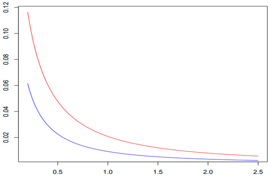
Figure 1. Comparison of tails $\overline{F_{X_{\left(\nu \right)}}}$ (blue line) and $\overline{F_{X_{\left(3\right)}}}$ (red line) from Example 3.

We note that Proposition 3 (i) can also be applied to other Burr type XII distributions whose distribution functions have the form

$$F\left(x\right)=\left(1-{\left(1+{\left(\frac{x}{\beta }\right)}^{\alpha }\right)}^{-\gamma }\right){\mathbb{I}}_{[0,\infty )}\left(x\right),$$

where $\alpha ,\beta ,\gamma$ are positive parameters; see [49], for instance.

Example 4. 

Let $\{X_1,X_2,\dots \}$ be a sequence of independent r.v.s such that $F_{X_1}$ is distributed according to the Weibull law with the scale parameter 1 and the shape parameter $1/2$, i.e.,

$$\overline{F_{X_1}}\left(x\right)={\mathbb{I}}_{(-\infty ,0)}\left(x\right)+{\mathrm{e}}^{-\sqrt{x}}{\mathbb{I}}_{[0,\infty )}\left(x\right).$$

Since $F_{X_1}\in \mathcal{H}$, due to Proposition 4 (i), we obtain that the d.f. of the randomly stopped minimum of sums $F_{S_{\left(\nu \right)}}$ is heavy-tailed and

$$\overline{F_{S_{\left(\nu \right)}}}\left(x\right)\underset{x\to \infty }{\asymp }\overline{F_{X_1}}\left(x\right)$$

if $\underset{2\le k\le \varkappa }{min}\mathbb{P}(X_k\ge 0)>0$ for $\varkappa =min\left\{\mathrm{supp}\right(\nu )\setminus \{0\left\}\right\}$.

For example, if

$$\mathbb{P}(X_k=-1)=\mathbb{P}(X_k=1)=\frac{1}{2},k\in \{2,3,\dots \},$$

and $\nu$ is distributed according to the shifted Poisson law (7), then $F_{S_{\left(\nu \right)}}\in \mathcal{H}$ and

$$\overline{F_{S_{\left(\nu \right)}}}\left(x\right)\underset{x\to \infty }{\asymp }{\mathrm{e}}^{-\sqrt{x}}.$$

A graphical representation of the last relation is shown in Figure 2, having in mind that

$$\frac{1}{4\mathrm{e}}{\mathrm{e}}^{-\sqrt{x}}\le \overline{F_{S_{\left(\nu \right)}}}\left(x\right)\le {\mathrm{e}}^{-\sqrt{x}},x\ge 0,$$

and

$$\overline{F_{S_{\left(\nu \right)}}}\left(x\right)=\frac{1}{\mathrm{e}}\sum _{n=3}^{\infty }\mathbb{P}\left(\bigcap _{k=1}^n\{S_k>x\}\right)\frac{1}{(n-3)!}=\frac{1}{\mathrm{e}}\sum _{n=3}^{\infty }\frac{{\mathrm{∆}}_n\left(x\right)}{(n-3)!},$$

where

$$\begin{array}{cc}\hfill {\mathrm{∆}}_{2m}\left(x\right)& =\frac{1}{2^{2m-1}}\sum _{k=0}^{m-1}\left(\genfrac{}{}{0pt}{}{2m-1}{k}\right)\left({\mathrm{e}}^{-\sqrt{x+2(m-k)-1}}+{\mathrm{e}}^{-\sqrt{x+2(m-k)-2}}\right),m\in \{2,3,\cdots \};\hfill \\ \hfill {\mathrm{∆}}_{2m+1}\left(x\right)& =\frac{1}{2^{2m}}\sum _{k=0}^{m-1}\left(\genfrac{}{}{0pt}{}{2m}{k}\right)\left({\mathrm{e}}^{-\sqrt{x+2(m-k)}}+{\mathrm{e}}^{-\sqrt{x+2(m-k)-1}}\right)\hfill \\ \hfill & +\frac{1}{2^{2m}}\left(\genfrac{}{}{0pt}{}{2m}{m}\right){\mathrm{e}}^{-\sqrt{x}},m\in \{1,2,\dots \}.\hfill \end{array}$$

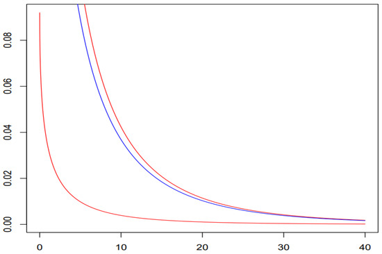
Figure 2. Tail of d.f. $\overline{F_{S_{\left(\nu \right)}}}$ (blue line) and its bounds (red lines) from Example 4.

5. Proofs of the Main Results

In this section, we present the proofs of all main propositions. We assign a separate subsection to the proof of each proposition.

5.1. Proof of Proposition 1

Proof of part (i). 

For any $\lambda >0$ and an arbitrary $K\ge 1$, we have

$$\begin{array}{cc}\hfill \mathbb{E}{\mathrm{e}}^{\lambda S_{\nu }}& =\mathbb{E}\left({\mathrm{e}}^{\lambda S_{\nu }}\sum _{n=0}^{\infty }{\mathbb{1}}_{\{\nu =n\}}\right)=\mathbb{E}\left(\sum _{n=0}^{\infty }{\mathrm{e}}^{\lambda S_n}{\mathbb{1}}_{\{\nu =n\}}\right)\hfill \\ & \ge \mathbb{E}\left(\sum _{n=0}^K{\mathrm{e}}^{\lambda S_n}{\mathbb{1}}_{\{\nu =n\}}\right)\hfill \\ \hfill & =\sum _{n=0}^K\mathbb{E}{\mathrm{e}}^{\lambda S_n}\mathbb{P}(\nu =n).\hfill \end{array}$$

(9)

From the condition

$$\underset{k\ge 1}{inf}\mathbb{E}{\mathrm{e}}^{\lambda X_k}>1$$

we derive that the estimate

$$\underset{1\le k\le K}{min}\mathbb{E}{\mathrm{e}}^{\lambda X_k}\ge \mathrm{∆}$$

holds for some $\mathrm{∆}=\mathrm{∆}\left(\lambda \right)>1$. Therefore, for all $n\in \{1,\dots ,K\}$, we obtain

$$\begin{array}{c}\hfill \mathbb{E}{\mathrm{e}}^{\lambda S_n}=\prod _{k=1}^n\mathbb{E}{\mathrm{e}}^{\lambda X_k}\ge {\mathrm{∆}}^n.\end{array}$$

(10)

This, together with (9), implies that

$$\begin{array}{c}\hfill \mathbb{E}{\mathrm{e}}^{\lambda S_{\nu }}\ge \sum _{n=0}^K{\mathrm{∆}}^n\mathbb{P}(\nu =n).\end{array}$$

Since $F_{\nu }\in \mathcal{H}$, we have

$$\begin{array}{cc}\hfill \sum _{n=0}^K{\mathrm{∆}}^n\mathbb{P}(\nu =n)& =\mathbb{E}{\mathrm{e}}^{\nu log\mathrm{∆}}{\mathbb{I}}_{\{\nu \le K\}}\underset{K\to \infty }{\to }\infty .\hfill \end{array}$$

Hence, $\mathbb{E}{\mathrm{e}}^{\lambda S_{\nu }}=\infty$ implying $F_{S_{\nu }}\in \mathcal{H}$ by definition. Part (i) of the proposition is proved. □

Proof of part (ii). 

Let us fix an arbitrary $\lambda >0$. Due to the conditions of part (ii), for such $\lambda$, we have

$$\begin{array}{cc}\hfill \underset{k\ge 1}{inf}\mathbb{E}{\mathrm{e}}^{\lambda X_k}& =\underset{k\ge 1}{inf}\left(\mathbb{E}{\mathrm{e}}^{\lambda X_k}{\mathbb{1}}_{\{X_k\ge a\}}+\mathbb{E}{\mathrm{e}}^{\lambda X_k}{\mathbb{1}}_{\{X_k<a\}}\right)\hfill \\ \hfill & \ge \underset{k\ge 1}{inf}\mathbb{E}{\mathrm{e}}^{\lambda X_k}{\mathbb{1}}_{\{X_k\ge a\}}\hfill \\ \hfill & \ge \underset{k\ge 1}{inf}{\mathrm{e}}^{\lambda a}\mathbb{P}(X_k\ge a)\hfill \\ \hfill & ={\mathrm{e}}^{\lambda a}>1.\hfill \end{array}$$

Hence, the assertion of part (ii) follows from part (i) of the proposition. □

Proof of part (iii). 

The requirement $\overline{F_{\nu }}\left(x\right)>0$ for all $x\in \mathbb{R}$ implies that counting r.v. $\nu$ has an unbounded support. Thus, we can find $K\ge \varkappa$ such that $\mathbb{P}(\nu =K)>0$. Let $\lambda$ be any positive number and $M\ge 1$. Then,

$$\begin{array}{cc}\hfill \mathbb{E}{\mathrm{e}}^{\lambda S_K}& \ge \mathbb{E}exp\left\{\lambda \sum _{k=1}^K{X}_k{\mathbb{I}}_{\{X_k\le M\}}\right\}\hfill \\ \hfill & =\mathbb{E}{\mathrm{e}}^{\lambda X_{\varkappa }{\mathbb{I}}_{\{X_{\varkappa }\le M\}}}\prod _{\begin{array}{c}k=1\\ k\ne \varkappa \end{array}}^K\mathbb{E}{\mathrm{e}}^{\lambda X_k{\mathbb{I}}_{\{X_k\le M\}}}\underset{M\to \infty }{\to }\infty \hfill \end{array}$$

because $F_{\varkappa }\in \mathcal{H}$ and $\mathbb{E}{\mathrm{e}}^{\lambda X_k}>0$ for each $k\in \{1,\dots ,K\}$. Therefore, $F_{S_K}\in \mathcal{H}$. By representation (9), we obtain that

$$\begin{array}{c}\hfill \mathbb{E}{\mathrm{e}}^{\lambda S_{\nu }}\ge \mathbb{P}(\nu =K)\mathbb{E}{\mathrm{e}}^{\lambda S_K}\end{array}$$

implying $F_{S_{\nu }}\in \mathcal{H}$. This completes the proof of part (iii) of the proposition. □

Proof of part (iv). 

Let K be such that $\mathbb{P}(\nu =K)>0$ and $\varkappa \le K$. Clearly, the conditions of part (iv) imply the existence of such K. To finish the proof of this part, it is sufficient to repeat the arguments of part (iii). □

Proof of part (v). 

Suppose that $0<\delta \le \lambda$, and $\lambda >0$ is such that $\mathbb{E}{\mathrm{e}}^{\lambda X_1^{+}}<\infty$ with $X_1^{+}:=X_1{\mathbb{I}}_{\{X_1\ge 0\}}$. By the standard representation (9), we have

$$\begin{array}{cc}\hfill \mathbb{E}{\mathrm{e}}^{\delta S_{\nu }}& =\sum _{n=0}^{\infty }\mathbb{E}{\mathrm{e}}^{\delta S_n}\mathbb{P}(\nu =n)\hfill \\ \hfill & \le \sum _{n=0}^{\infty }\mathbb{E}{\mathrm{e}}^{\delta S_n^{+}}\mathbb{P}(\nu =n),\hfill \end{array}$$

(11)

where $S_0^{+}=0$ and

$$S_n^{+}=\sum _{k=1}^n{X}_k^{+}=\sum _{k=1}^n{X}_k{\mathbb{I}}_{\{X_k\ge 0\}},n\in \{1,2,\dots \}.$$

Condition (4) implies

$$\begin{array}{c}\hfill \overline{F_{X_k}}\left(x\right)\le c_1\overline{F_{X_1}}\left(x\right)\end{array}$$

(12)

for some $c_1>0$, all $k\ge 1$ and all $x\in \mathbb{R}$. Therefore, by the alternative expectation formula (see, for instance, [45]), we derive from (12) that

$$\begin{array}{cc}\hfill \mathbb{E}{\mathrm{e}}^{\delta X_k^{+}}& =1+\delta {\int }_0^{\infty }{\mathrm{e}}^{\delta u}\overline{F_{X_k^{+}}}\left(u\right)\mathrm{d}u\hfill \\ \hfill & \le 1+\delta c_1{\int }_0^{\infty }{\mathrm{e}}^{\lambda u}\overline{F_{X_1}}\left(u\right)\mathrm{d}u\hfill \\ \hfill & =1+\frac{\delta }{\lambda }{c}_1\left(\mathbb{E}{\mathrm{e}}^{\lambda X_1^{+}}-1\right):=c_2\left(\delta \right)\hfill \end{array}$$

for any $k\ge 1$, where $1<c_2\left(\delta \right)<\infty$ for $0<\delta \le \lambda$, and

$$\underset{\delta \downarrow 0}{lim}{c}_2\left(\delta \right)=1.$$

Since $X_1^{+},X_2^{+},\dots$ are independent r.v.s, we obtain

$$\mathbb{E}{\mathrm{e}}^{\delta S_n^{+}}=\prod _{k=1}^n\mathbb{E}{\mathrm{e}}^{\delta X_k^{+}}\le {\left(c_2\left(\delta \right)\right)}^n.$$

Hence, by inequality (11) and condition $F_{\nu }\in {\mathcal{H}}^c$ we derive that

$$\mathbb{E}{\mathrm{e}}^{\delta S_{\nu }}\le \sum _{n=0}^{\infty }{\left(c_2\left(\delta \right)\right)}^n\mathbb{P}(\nu =n)=\mathbb{E}{\mathrm{e}}^{\nu log{c}_2\left(\delta \right)}<\infty$$

if $\delta \in (0,\lambda ]$ is chosen as sufficiently small.

This implies that $F_{S_{\nu }}\in {\mathcal{H}}^c$. □

Proof of part (vi). 

The statement of this part can be proved analogously to the statement of part (v). Namely, the conditions of part (vi) imply that

$$\underset{k\ge 1}{sup}\mathbb{E}{\mathrm{e}}^{\lambda X_k^{+}}=c_{\lambda }$$

for some constants $\lambda >0$ and $c_{\lambda }\ge 1$. Therefore, using the alternative expectation formula, we derive

$$\begin{array}{cc}\hfill \mathbb{E}{\mathrm{e}}^{\delta X_k^{+}}& =1+\delta {\int }_{[0,\infty )}{\mathrm{e}}^{\delta u}\overline{F_{X_k}}\left(u\right)\mathrm{d}u\hfill \\ \hfill & \le 1+\frac{\delta }{\lambda }\left(\lambda {\int }_{[0,\infty )}{\mathrm{e}}^{\lambda u}\overline{F_{X_k}}\left(u\right)\mathrm{d}u\right)\hfill \\ \hfill & =1+\frac{\delta }{\lambda }\left(c_{\lambda }-1\right)\hfill \end{array}$$

for all $\delta \in (0,\lambda )$ and $k\ge 1$. The last estimation and inequality (11) imply that

$$\mathbb{E}{\mathrm{e}}^{\delta S_{\nu }}\le \sum _{n=0}^{\infty }\prod _{k=1}^n\mathbb{E}{\mathrm{e}}^{\delta X_k^{+}}\mathbb{P}(\nu =n)\le \mathbb{E}{\mathrm{e}}^{\nu log\left(1+\frac{\delta }{\lambda }(c_{\lambda }-1)\right)}.$$

If $\delta \in (0,\lambda ]$ is sufficiently small, then the last expectation is finite because of $F_{\nu }\in {\mathcal{H}}^c$. Hence, $F_{S_{\nu }}\in {\mathcal{H}}^c$ as well. Part (vi) of the proposition is proved. □

5.2. Proof of Proposition 2

Proof of part (ii). 

By the standard representation, we have

$$\begin{array}{cc}\hfill \overline{F_{X^{\left(\nu \right)}}}\left(x\right)& =\sum _{n=1}^{\infty }\mathbb{P}(X^{\left(n\right)}>x)\mathbb{P}(\nu =n)\hfill \\ \hfill & \ge \mathbb{P}(X^{\left(K\right)}>x)\mathbb{P}(\nu =K)\hfill \end{array}$$

(13)

for $x>0$ and any K such that $\mathbb{P}(\nu =K)>0$, $K\ge \varkappa$. Due to the conditions of part (ii), there exists a sequence of numbers K with the above property. Obviously,

$$\begin{array}{cc}\hfill \mathbb{P}(X^{\left(K\right)}>x)& =\mathbb{P}(max\{0,X_1,\dots ,X_K\}>x)\hfill \\ \hfill & \ge \mathbb{P}(X_{\varkappa }>x).\hfill \end{array}$$

(14)

Consequently, for an arbitrary $\lambda >0$, we obtain from (13) and (14)

$$\underset{x\to \infty }{lim\; sup}{\mathrm{e}}^{\lambda x}\overline{F_{X^{\left(\nu \right)}}}\left(x\right)\ge \mathbb{P}(\nu =K)\underset{x\to \infty }{lim\; sup}{\mathrm{e}}^{\lambda x}\overline{F_{X_{\varkappa }}}\left(x\right).$$

The assertion of part (i) follows now by Lemma 1. □

Proof of part (ii). 

The proof of this part is similar to the proof of part (i), because the conditions of part (ii) imply that there exists at least one K such that $K\ge \varkappa$ and $\mathbb{P}(\nu =K)>0$. □

Proof of part (iii). 

The standard representation implies that

$$\begin{array}{cc}\hfill \overline{F_{X^{\left(\nu \right)}}}\left(x\right)& =\sum _{n=1}^{\infty }\mathbb{P}(X^{\left(n\right)}>x)\mathbb{P}(\nu =n)\hfill \\ & =\sum _{n=1}^{\infty }\mathbb{P}\left(\bigcup _{k=1}^n\{X_k>x\}\right)\mathbb{P}(\nu =n)\hfill \end{array}$$

(15)

$$\begin{array}{cc}\hfill & \le \sum _{n=1}^{\infty }\mathbb{P}(\nu =n)\sum _{k=1}^n\overline{F_{X_k}}\left(x\right)\hfill \end{array}$$

(16)

for positive x.

Due to Lemma 1, there is $\lambda >0$ such that

$$\begin{array}{c}\hfill \underset{x\to \infty }{lim\; sup}{\mathrm{e}}^{\lambda x}\overline{F_{X_1}}\left(x\right)<\infty .\end{array}$$

(17)

It follows from the estimate (15) that

$$\begin{array}{c}\hfill \underset{x\to \infty }{lim\; sup}{\mathrm{e}}^{\lambda x}\overline{F_{X^{\left(\nu \right)}}}\left(x\right)\le \underset{x\to \infty }{lim\; sup}{\mathrm{e}}^{\lambda x}\sum _{n=1}^{\infty }\mathbb{P}(\nu =n)\sum _{k=1}^n\overline{F_{X_k}}\left(x\right).\end{array}$$

Condition (5) of part (iii) implies that

$$\begin{array}{cc}\hfill \sum _{k=1}^n\overline{F_{X_k}}\left(x\right)& \le c_{4}n\overline{F_{X_1}}\left(x\right)\hfill \end{array}$$

(18)

for all $n\ge 1$, for some $c_4>0$ and for sufficiently large $x(x\ge x_1)$. Therefore, by (17) and (18), we obtain that

$$\begin{array}{c}\hfill \underset{x\to \infty }{lim\; sup}{\mathrm{e}}^{\lambda x}\overline{F_{X^{\left(\nu \right)}}}\left(x\right)\le c_4\mathbb{E}\nu \underset{x\to \infty }{lim\; sup}{\mathrm{e}}^{\lambda x}\overline{F_{X_1}}\left(x\right)<\infty .\end{array}$$

The assertion of part (iii) follows now by Lemma 1. □

5.3. Proof of Proposition 3

Proof of part (i). 

By the standard representation we have

$$\begin{array}{cc}\hfill \overline{F_{X_{\left(\nu \right)}}}\left(x\right)& =\sum _{n=1}^{\infty }\mathbb{P}\left(min\{X_1,\dots ,X_n\}>x\right)\mathbb{P}(\nu =n)\hfill \\ \hfill & =\sum _{n=1}^{\infty }\mathbb{P}(\nu =n)\prod _{k=1}^n\overline{F_{X_k}}\left(x\right)\hfill \\ \hfill & =\overline{F_{X_{\left(\varkappa \right)}}}\left(x\right)\mathbb{P}(\nu =\varkappa )+\sum _{n=\varkappa +1}^{\infty }\mathbb{P}(\nu =n)\overline{F_{X_{\left(\varkappa \right)}}}\left(x\right)\prod _{k=\varkappa +1}^n\overline{F_{X_k}}\left(x\right)\hfill \\ \hfill & \le \overline{F_{X_{\left(\varkappa \right)}}}\left(x\right)\mathbb{P}(\nu =\varkappa )\left(1+\overline{F_{X_{\varkappa +1}}}\left(x\right)\frac{\mathbb{P}(\nu >\varkappa )}{\mathbb{P}(\nu =\varkappa )}\right),\hfill \end{array}$$

(19)

and

$$\begin{array}{c}\hfill \overline{F_{X_{\left(\nu \right)}}}\left(x\right)\ge \overline{F_{X_{\left(\varkappa \right)}}}\left(x\right)\mathbb{P}(\nu =\varkappa )\end{array}$$

for each positive x. In addition, conditions of part (i) give that $\overline{F_{X_{\left(\varkappa \right)}}}\left(x\right)>0$ for all positive x. Therefore,

$$\begin{array}{c}\hfill \overline{F_{X_{\left(\nu \right)}}}\left(x\right)\underset{x\to \infty }{\sim }\mathbb{P}(\nu =\varkappa )\overline{F_{X_{\left(\varkappa \right)}}}\left(x\right).\end{array}$$

We obtain from this, by using Lemma 2, that $F_{X_{\left(\nu \right)}}\in \mathcal{H}$ if $F_{X_{\left(\varkappa \right)}}\in \mathcal{H}$. Hence, to prove the assertion of part (i) it is enough to prove that $F_{X_{\left(\varkappa \right)}}\in \mathcal{H}$ for $1\le \varkappa \le min\left\{\mathrm{supp}\right(\nu )\setminus \{0\left\}\right\}$.

Due to the condition $F_{X_1}\in \mathcal{H}$ and Lemma 1, we have

$$\underset{x\to \infty }{lim\; sup}{\mathrm{e}}^{\lambda x}\overline{F_{X_1}}\left(x\right)=\infty$$

(20)

for an arbitrary $\lambda >0$. The requirement

$$\underset{x\to \infty }{lim\; inf}\underset{1⩽k⩽\varkappa }{min}\frac{\overline{F_{X_k}}\left(x\right)}{\overline{F_{X_1}}\left(x\right)}>0$$

implies that

$$\overline{F_{X_k}}\left(x\right)\ge c_5\overline{F_{X_1}}\left(x\right)$$

for some positive $c_5$, sufficiently large x$(x\ge x_2)$ and for all $1\le k\le \varkappa$. Therefore, for any positive $\lambda$ and large $x(x\ge x_2)$ we obtain

$$\begin{array}{cc}\hfill {\mathrm{e}}^{\lambda x}\overline{F_{X_{\left(\varkappa \right)}}}\left(x\right)& ={\mathrm{e}}^{\lambda x}\prod _{k=1}^{\varkappa }\overline{F_{X_k}}\left(x\right)\hfill \\ \hfill & \ge c_5^{\varkappa }{\mathrm{e}}^{\lambda x}{\left(\overline{F_{X_1}}\left(x\right)\right)}^{\varkappa }\hfill \\ \hfill & ={\left(c_5{\mathrm{e}}^{\lambda x/\varkappa }\overline{F_{X_1}}\left(x\right)\right)}^{\varkappa }.\hfill \end{array}$$

By relation (20) we derive that

$$\underset{x\to \infty }{lim\; sup}{\mathrm{e}}^{\lambda x}\overline{F_{X_{\left(\varkappa \right)}}}\left(x\right)=\infty$$

implying that $F_{X_{\left(\varkappa \right)}}\in \mathcal{H}$. Part (i) of the proposition is proved. □

Proof of part (ii). 

According to inequality (19) and Lemma 2, $F_{X_{\left(\nu \right)}}\in {\mathcal{H}}^c$ if $F_{X_{\left(\varkappa \right)}}\in {\mathcal{H}}^c$. Since $\varkappa$ is finite, conditions $F_{X_k}\in {\mathcal{H}}^c$, $k\in \{1,2,\dots ,\varkappa \}$ and Lemma 1 imply that

$$\underset{x\to \infty }{lim\; sup}{\mathrm{e}}^{\lambda x}\overline{F_{X_k}}\left(x\right)<\infty$$

(21)

for some $\lambda >0$ and each $k\in \{1,2,\dots ,\varkappa \}$. For this $\lambda$ and an arbitrary positive x, we have

$${\mathrm{e}}^{\lambda x}\overline{F_{X_{\left(\varkappa \right)}}}\left(x\right)=\prod _{k=1}^{\varkappa }\left({\mathrm{e}}^{\lambda x/\varkappa }\overline{F_{X_k}}\left(x\right)\right).$$

Since $\lambda /\varkappa \le \lambda$, due to (21),

$$\underset{x\to \infty }{lim\; sup}{\mathrm{e}}^{\lambda x/\varkappa }\overline{F_{X_k}}\left(x\right)<\infty$$

for each $k\in \{1,2,\dots ,\varkappa \}$. Therefore,

$$\underset{x\to \infty }{lim\; sup}{\mathrm{e}}^{\lambda x}\overline{F_{X_{\left(\varkappa \right)}}}\left(x\right)<\infty$$

implying that $F_{X_{\left(\varkappa \right)}}\in {\mathcal{H}}^c$ by Lemma 1. Hence, $F_{X_{\left(\nu \right)}}\in {\mathcal{H}}^c$ as well, and part (ii) of the proposition is proved. □

5.4. Proof of Proposition 4

Proof of part (i). 

If $\varkappa =1$, then for $x>0$, we have

$$\begin{array}{cc}\hfill \overline{F_{S_{\left(\nu \right)}}}\left(x\right)& =\sum _{n\in \mathrm{supp}\left(\nu \right)\setminus \left\{0\right\}}\overline{F_{S_{\left(n\right)}}}\left(x\right)\mathbb{P}(\nu =n)\hfill \\ \hfill & \ge \overline{F_{S_{\left(1\right)}}}\left(x\right)\mathbb{P}(\nu =1)\hfill \\ \hfill & =\overline{F_{X_1}}\left(x\right)\mathbb{P}(\nu =1),\hfill \end{array}$$

and

$$\begin{array}{cc}\hfill \overline{F_{S_{\left(\nu \right)}}}\left(x\right)& =\sum _{n=1}^{\infty }\overline{F_{S_{\left(n\right)}}}\left(x\right)\mathbb{P}(\nu =n)\hfill \\ \hfill & =\sum _{n=1}^{\infty }\mathbb{P}\left(min\{S_1,\cdots ,S_n\}>x\right)\mathbb{P}(\nu =n)\hfill \\ \hfill & =\sum _{n=1}^{\infty }\mathbb{P}\left(\bigcap _{k=1}^n\{S_k>x\}\right)\mathbb{P}(\nu =n)\hfill \\ \hfill & \le \sum _{n=1}^{\infty }\mathbb{P}(S_1>x)\mathbb{P}(\nu =n)\hfill \\ \hfill & =\overline{F_{X_1}}\left(x\right)\mathbb{P}(\nu \ge 1).\hfill \end{array}$$

The derived estimates imply the asymptotic relation (6) in the case $\varkappa =1$.

Let us now suppose that $\varkappa >1$. Due to the conditions of part (i)

$$\begin{array}{c}\hfill \mathbb{P}(X_k\ge 0)\ge c_6\end{array}$$

for some $c_6>0$ and all $1\le k\le \varkappa$. Hence, by the standard decomposition, we obtain that for positive x

$$\begin{array}{cc}\hfill \overline{F_{S_{\left(\nu \right)}}}\left(x\right)& =\sum _{n=1}^{\infty }{\overline{F}}_{S_{\left(n\right)}}\left(x\right)\mathbb{P}(\nu =n)\hfill \\ \hfill & \ge \overline{F_{S_{\left(\varkappa \right)}}}\left(x\right)\mathbb{P}(\nu =\varkappa )\hfill \\ \hfill & =\mathbb{P}\left(min\{S_1,\cdots ,S_{\varkappa }\}>x\right)\mathbb{P}(\nu =\varkappa )\hfill \\ \hfill & =\mathbb{P}\left(\bigcap _{k=1}^{\varkappa }\{X_1+\dots +X_k>x\}\right)\mathbb{P}(\nu =\varkappa )\hfill \\ \hfill & \ge \mathbb{P}\left(X_1>x,X_2\ge 0,\dots ,X_{\varkappa }\ge 0\right)\mathbb{P}(\nu =\varkappa )\hfill \\ \hfill & =\mathbb{P}(X_1>x)\prod _{k=2}^{\varkappa }\mathbb{P}(X_k\ge 0)\mathbb{P}(\nu =\varkappa )\hfill \\ \hfill & \ge c_6^{\varkappa -1}\mathbb{P}(\nu =\varkappa )\overline{F_{X_1}}\left(x\right).\hfill \end{array}$$

(22)

On the other hand, similarly, as in the case $\varkappa =1$, we have

$$\begin{array}{cc}\hfill \overline{F_{S_{\left(\nu \right)}}}\left(x\right)& =\sum _{n\in \mathrm{supp}\left(\nu \right)\setminus \left\{0\right\}}\mathbb{P}\left(\bigcap _{k=1}^n\{S_k>x\}\right)\mathbb{P}(\nu =n)\hfill \\ \hfill & \le \sum _{n\in \mathrm{supp}\left(\nu \right)\setminus \left\{0\right\}}\mathbb{P}(S_1>x)\mathbb{P}(\nu =n)\hfill \\ \hfill & =\overline{F_{X_1}}\left(x\right)\mathbb{P}(\nu \ge \varkappa ).\hfill \end{array}$$

(23)

Estimates (22) and (23) imply that the asymptotic relation (6) holds for any possible $\varkappa$. In addition, we observe that, by Lemma 2, distribution $F_{S_{\left(\nu \right)}}$ belongs to $\mathcal{H}$ together with $F_{X_1}$. Part (i) of the proposition is proved. □

Proof of part (ii). 

The statement of this part follows immediately from the estimate (23) and Lemma 1 because

$$\begin{array}{c}\hfill \underset{x\to \infty }{lim\; sup}{\mathrm{e}}^{\lambda x}\overline{F_{S_{\left(\nu \right)}}}\left(x\right)\le \mathbb{P}(\nu \ge 1)\underset{x\to \infty }{lim\; sup}{\mathrm{e}}^{\lambda x}\overline{F_{X_1}}\left(x\right)\end{array}$$

for any $\lambda >0$. □

5.5. Proof of Proposition 5

Proof of part (i). 

Proof of this part is similar to the proof of part (i) of Proposition 1. Namely, for $\lambda >0$ and $K\ge 2$ by using (10), we obtain that

$$\begin{array}{cc}\hfill \mathbb{E}{\mathrm{e}}^{\lambda S^{\left(\nu \right)}}& \ge \mathbb{E}\left({\mathrm{e}}^{\lambda S^{\left(\nu \right)}}{\mathbb{1}}_{\{\nu \le K\}}\right)\hfill \\ \hfill & =\sum _{n=0}^K\mathbb{E}{\mathrm{e}}^{\lambda S^{\left(n\right)}}\mathbb{P}(\nu =n)\hfill \\ \hfill & \ge \sum _{n=0}^K\mathbb{E}{\mathrm{e}}^{\lambda S_n}\mathbb{P}(\nu =n)\hfill \\ \hfill & \ge \sum _{n=0}^K{\mathrm{∆}}^n\mathbb{P}(\nu =n)\hfill \\ \hfill & =\mathbb{E}\left({\mathrm{e}}^{\nu log\mathrm{∆}}{\mathbb{1}}_{\{\nu \le K\}}\right)\hfill \end{array}$$

with $\mathrm{∆}=\mathrm{∆}\left(\lambda \right)=\underset{k\ge 1}{inf}\mathbb{E}{\mathrm{e}}^{\lambda X_k}>1$. The condition $F_{\nu }\in \mathcal{H}$ implies that

$$\begin{array}{c}\hfill \underset{K\to \infty }{lim}\mathbb{E}\left({\mathrm{e}}^{\nu log\mathrm{∆}}{\mathbb{1}}_{\{\nu \le K\}}\right)=\infty .\end{array}$$

Therefore, $\mathbb{E}{\mathrm{e}}^{\lambda S^{\left(\nu \right)}}=\infty$ for an arbitrary $\lambda >0$, i.e., $F_{S^{\left(\nu \right)}}\in \mathcal{H}$. Part (i) of the proposition is proved. □

Proof of part (ii). 

The assertion of this part is obvious because condition $\underset{k\ge 1}{inf}\mathbb{P}(X_k\ge a)=1$ with $a>0$ implies that $\underset{k\ge 1}{inf}\mathbb{E}{\mathrm{e}}^{\lambda X_k}>1$ for any $\lambda >0$. The details of this implication are presented in the proof of Proposition 1 (ii). □

Proof of part (iii). 

For positive x, we have

$$\begin{array}{cc}\hfill \overline{F_{S^{\left(\nu \right)}}}\left(x\right)& =\sum _{n=1}^{\infty }\overline{F_{S^{\left(n\right)}}}\left(x\right)\mathbb{P}(\nu =n)\hfill \\ \hfill & =\sum _{n=1}^{\infty }\mathbb{P}\left(\bigcup _{k=1}^n\{S_k>x\}\right)\mathbb{P}(\nu =n)\hfill \\ \hfill & \ge \sum _{n=1}^{\infty }\mathbb{P}(S_1>x)\mathbb{P}(\nu =n)\hfill \\ \hfill & =\overline{F_{X_1}}\left(x\right)\mathbb{P}(\nu \ge 1).\hfill \end{array}$$

(24)

The assertion of part (iii) follows now from Lemma 1 because by (24)

$$\underset{x\to \infty }{lim\; sup}{\mathrm{e}}^{\lambda x}\overline{F_{S^{\left(\nu \right)}}}\left(x\right)\ge \mathbb{P}(\nu \ge 1)\underset{x\to \infty }{lim\; sup}{\mathrm{e}}^{\lambda x}\overline{F_{X_1}}\left(x\right)$$

for an arbitrary positive $\lambda$. □

Proof of part (iv). 

Conditions of this part and and Proposition 1 (parts (iii) and (iv)) imply that $F_{S_{\nu }}\in \mathcal{H}$. In addition, for positive x,

$$\begin{array}{cc}\hfill \overline{F_{S^{\left(\nu \right)}}}\left(x\right)& =\sum _{n=1}^{\infty }\mathbb{P}\left(max\{S_1,S_2,\dots ,S_n\}>x\right)\mathbb{P}(\nu =n)\hfill \\ & \ge \sum _{n=1}^{\infty }\mathbb{P}(S_n>x)\mathbb{P}(\nu =n)\hfill \\ \hfill & =\overline{F_{S_{\nu }}}\left(x\right).\hfill \end{array}$$

Hence, $F_{S^{\left(\nu \right)}}\in \mathcal{H}$, according to the Lemma 2. Part (iv) of the proposition is proved. □

Proof of part (v). 

Let $\lambda >0$ be a positive number from the condition of part (v), i.e.,

$$\underset{k\ge 1}{sup}\mathbb{E}{\mathrm{e}}^{\lambda X_k}={\widehat{c}}_{\lambda }$$

with some positive constant ${\widehat{c}}_{\lambda }$. For this $\lambda$, we have

$$\begin{array}{cc}\hfill \underset{k\ge 1}{sup}\mathbb{E}{\mathrm{e}}^{\lambda X_k^{+}}& =\underset{k\ge 1}{sup}\mathbb{E}\left({\mathrm{e}}^{\lambda X_k^{+}}{\mathbb{1}}_{\{X_k\ge 0\}}+{\mathrm{e}}^{\lambda X_k^{+}}{\mathbb{1}}_{\{X_k<0\}}\right)\hfill \\ \hfill & =\underset{k\ge 1}{sup}\mathbb{E}\left({\mathrm{e}}^{\lambda X_k}{\mathbb{1}}_{\{X_k\ge 0\}}+{\mathbb{1}}_{\{X_k<0\}}\right)\hfill \\ \hfill & \le {\widehat{c}}_{\lambda }+1,\hfill \end{array}$$

where $X_k^{+}=X_k{\mathbb{I}}_{\{X_k\ge 0\}}$ for $k\in \{1,2,\dots ,\}$. Due to Proposition 1(vi), d.f. $F_{S_{\nu }^{+}}$ belongs to the class ${\mathcal{H}}^c$ with r.v. $S_{\nu }^{+}=X_1^{+}+\dots +X_{\nu }^{+}$.

According to the standard representation, for positive x, we have

$$\begin{array}{cc}\hfill \overline{F_{S^{\left(\nu \right)}}}\left(x\right)& =\sum _{n=1}^{\infty }\mathbb{P}\left(max\{S_1,S_2,\dots ,S_n\}>x\right)\mathbb{P}(\nu =n)\hfill \\ \hfill & \le \sum _{n=1}^{\infty }\mathbb{P}\left(max\{S_1^{+},S_2^{+},\dots ,S_n^{+}\}>x\right)\mathbb{P}(\nu =n)\hfill \\ \hfill & =\sum _{n=1}^{\infty }\mathbb{P}(S_n^{+}>x)\mathbb{P}(\nu =n)\hfill \\ \hfill & =\overline{F_{S_{\nu }^{+}}}\left(x\right).\hfill \end{array}$$

By applying Lemma 2, we obtain that d.f. $F_{S^{\left(\nu \right)}}$ is light-tailed due to the light tail of d.f. $F_{S_{\nu }^{+}}$. Part (v) of the proposition is proved. □

6. Concluding Remarks

In this paper, we show that both heavy-tailed and light-tailed classes of distributions have quite a number of interesting properties related to the randomly stopped structures. Based on our results, various heavy-tailed or light-tailed distributions can be constructed. On the other hand, according to the propositions we proved, in most cases, it is easier to determine whether the considered distribution is light-tailed or heavy-tailed. The main novelty of our work consists in the fact that we study randomly stopped structures in a set of independent but possibly differently distributed primary random variables. In Section 1, it was mentioned that randomly stopped structures together with heavy-tailed distributions appear in such fields as insurance and financial activity, survival analysis, risk management, computer and communication networks, etc. Recently, many articles have been written on the heavy-tailed distributions, both in scientific and popular science journals. Let us mention a few such works. Heavy-tailed distributions applied to financial losses and stochastic returns are described and discussed in [50,51,52]. The influence of heavy-tailed distributions on actuarial statistics is examined in [53,54,55,56]. The performance of heavy-tailed distributions in social and medical research is discussed in [57,58]. The application of heavy-tailed distributions of a special form to study computer systems and telecommunication networks is presented in [59,60,61]. More concretely, the results of the current paper related to the randomly stopped sums are applied not only to the standard areas such as insurance models ([62,63], etc.), but also to information ranking algorithms ([64,65]) and teletraffic arrivals [66].

From the content of the mentioned works, it can be seen that in many cases, it is quite difficult to fit heavy-tailed distributions to the real data. Therefore, our proposed transformations of heavy-tailed distributions increase the chances of choosing the right distribution. So, in our opinion, it makes sense to continue research on transformations for heavy-tailed distributions. In addition to the randomly stopped structures examined in this paper, moment transformations, random effects, and randomly stopped products can be considered, for instance.

References

- Albin, J.M.P. A note on the closure of covolution power mixtures (random sums) of exponential distributions. J. Aust. Math. Soc. 2008, 84, 1–7. [Google Scholar] [CrossRef][Green Version]
- Andrulytė, I.M.; Manstavičius, M.; Šiaulys, J. Randomly stopped maximum and maximum of sums with consistently varying distributions. Mod. Stoch. Theory Appl. 2017, 4, 65–78. [Google Scholar] [CrossRef][Green Version]
- Cheng, D.; Ni, F.; Pakes, A.G.; Wang, Y. Some properties of the exponential distribution class with application to risk theory. J. Korean Stat. Soc. 2012, 41, 515–527. [Google Scholar] [CrossRef]
- Cline, D.B.H. Convolutions of the distributions with exponential tails. J. Aust. Math. Soc. 1987, 43, 347–365. [Google Scholar] [CrossRef]
- Danilenko, S.; Šiaulys, J. Random convolution of O-exponential distributions. Nonlinear Anal. Model. 2015, 20, 447–454. [Google Scholar] [CrossRef]
- Danilenko, S.; Šiaulys, J. Randomly stopped sums of not identically distributed heavy tailed random variables. Stat. Probab. Lett. 2016, 113, 84–93. [Google Scholar] [CrossRef]
- Danilenko, S.; Markevičiūtė, J.; Šiaulys, J. Randomly stopped sums with exponential-type distributions. Nonlinear Anal. Model. 2017, 22, 793–807. [Google Scholar] [CrossRef]
- Danilenko, S.; Paškauskaitė, S.; Šiaulys, J. Random convolution of inhomogeneous distributions with O-exponential tail. Mod. Stoch. Theory Appl. 2016, 3, 79–94. [Google Scholar] [CrossRef][Green Version]
- Danilenko, S.; Šiaulys, J.; Stepanauskas, G. Closure properties of O-exponential distributions. Stat. Probab. Lett. 2018, 140, 63–70. [Google Scholar] [CrossRef]
- Dirma, M.; Nakliuda, N.; Šiaulys, J. Generalized moments of sums with heavy-tailed random summands. Lith. Math. J. 2023, 63, 254–271. [Google Scholar] [CrossRef]
- Embrechts, P.; Goldie, C.M. On the closure and factorization properties of subexponential and related distributions. J. Aust. Math. Soc. Ser. A 1980, 29, 243–256. [Google Scholar] [CrossRef]
- Geng, B.; Liu, Z.; Wang, S. A Kesten-type inequality for randomly weighted sums of dependent subexponential random variables with applications to risk theory. Lith. Math. J. 2023, 63, 81–91. [Google Scholar] [CrossRef]
- Karasevičienė, J.; Šiaulys, J. Randomly stopped sums with generalized subexponential distribution. Axioms 2023, 12, 641. [Google Scholar] [CrossRef]
- Karasevičienė, J.; Šiaulys, J. Randomly stopped minimum, maximum, minimum of sums and maximum of sums with generalized subexponential distributions. Axioms 2024, 13, 85. [Google Scholar] [CrossRef]
- Kizinevič, E.; Sprindys, J.; Šiaulys, J. Randomly stopped sums with consistently varying distributions. Mod. Stoch. Theory Appl. 2016, 3, 165–179. [Google Scholar] [CrossRef][Green Version]
- Konstantinides, D.; Leipus, R.; Šiaulys, J. A note on product-convolution for generalized subexponential distributions. Nonlinear Anal. Model. 2022, 27, 11054–11067. [Google Scholar] [CrossRef]
- Konstantinides, D.; Leipus, R.; Šiaulys, J. On the non-closure under convolution for strong subexponential distributions. Nonlinear Anal. Model. 2023, 28, 97–115. [Google Scholar] [CrossRef]
- Leipus, R.; Šiaulys, J. Closure of some heavy-tailed distribution classes under random convolution. Lith. Math. J. 2012, 52, 249–258. [Google Scholar] [CrossRef]
- Leipus, R.; Šiaulys, J. On the random max-closure for heavy-tailed random variables. Lith. Math. J. 2017, 57, 208–221. [Google Scholar] [CrossRef]
- Lin, J.; Wang, Y. New examples of heavy-tailed O-subexponenial distributions and related closure properties. Stat. Probab. Lett. 2012, 82, 427–432. [Google Scholar] [CrossRef]
- Ragulina, O.; Šiaulys, J. Randomly stopped minima and maxima with exponential-type distributions. Nonlinear Anal. Model. 2019, 24, 297–313. [Google Scholar] [CrossRef]
- Shimura, T.; Watanabe, T. Infinite divisibility and generalized subexponentiality. Bernoulli 2005, 11, 445–469. [Google Scholar] [CrossRef]
- Sprindys, J.; Šiaulys, J. Regularly distributed randomly stopped sum, minimum and maximum. Nonlinear Anal. Model. 2020, 25, 509–522. [Google Scholar] [CrossRef]
- Teicher, H. Moments of randomly stopped sums revisited. J. Theor. Probab. 1995, 8, 779–793. [Google Scholar] [CrossRef]
- Tesemnikov, P.I. On the distribution tail of the sum of the maxima of two randomly sums in the presence of heavy tails. Sib. Elektron. Mat. Izv. 2019, 16, 1785–1794. [Google Scholar] [CrossRef]
- Watanabe, T. Convolution equivalence and distributions of random sums. Probab. Theory Relat. Fields 2008, 142, 367–397. [Google Scholar] [CrossRef]
- Watanabe, T. The Wiener condition and the conjectures of Embrechts and Goldie. Ann. Probab. 2019, 47, 1221–1239. [Google Scholar] [CrossRef]
- Watanabe, T.; Yamamuro, K. Ratio of the tail of an infinity divisible distribution on the line to that of its Lévy measure. Electron. J. Probab. 2010, 15, 44–74. [Google Scholar] [CrossRef]
- Xu, H.; Foss, S.; Wang, Y. Convolution and convolution-root properties of long-tailed distributions. Extremes 2015, 18, 605–628. [Google Scholar] [CrossRef]
- Xu, H.; Wang, Y.; Cheng, D.; Yu, C. On the closure under infinitely divisible distribution roots. Lith. Math. J. 2022, 62, 258–287. [Google Scholar] [CrossRef]
- Markovich, N.M.; Rodionov, I.V. Maxima and sums of non-stationary random length sequences. Extremes 2020, 23, 451–464. [Google Scholar] [CrossRef]
- Leipus, R.; Šiaulys, J.; Konstantinides, D. Minimum of heavy-tailed random variables is not heavy-tailed. AIMS Math. 2023, 8, 13066–13072. [Google Scholar] [CrossRef]
- Andersen, E.S. On the collective theory of Risk in case of contagion between claims. Bull. Inst. Math. Appl. 1957, 12, 275–279. [Google Scholar]
- Asmussen, S.; Albrecher, H. Ruin Probabilities, 2nd ed.; Word Scientific: Singapore, 2010. [Google Scholar]
- Denisov, D.; Foss, S.; Korshunov, D. Tail asymptotics for the supremum of random walk when the mean is not finite. Queuing Syst. 2004, 46, 15–33. [Google Scholar] [CrossRef]
- Embrechts, P.; Klüppelberg, C.; Mikosch, T. Modelling Extremal Events for Insurance and Finance; Springer: New York, NY, USA, 1997. [Google Scholar]
- Embrechts, P.; Veraverbeke, N. Estimates for the probability of ruin with special emphasis and the possibility of large claims. Insur. Math. Econ. 1982, 1, 55–72. [Google Scholar] [CrossRef]
- Klüppelberg, C. Subexponential distributions and integrated tails. J. Appl. Probab. 1988, 25, 132–141. [Google Scholar] [CrossRef]
- Bingham, N.H.; Goldie, C.M.; Teugels, J.L. Regular Variation; Cambridge University Press: Cambridge, UK, 1987. [Google Scholar]
- Borovkov, A.A.; Borovkov, K.A. Asymptotic Analysis of Random Walks: Heavy-Tailed Distributions; Cambridge University Press: Cambridge, UK, 2008. [Google Scholar]
- Foss, S.; Korshunov, D.; Zachary, S. An Introduction to Heavy-Tailed and Subexponential Distributions, 2nd ed.; Springer: New York, NY, USA, 2013. [Google Scholar]
- Konstantinides, D.G. Risk Theory: A Heavy Tail Approach; World Scientific: Hackensack, NJ, USA, 2018. [Google Scholar]
- Leipus, R.; Šiaulys, J.; Konstantinides, D. Closure Properties for Heavy-Tailed and Related Distributions: An Overview; Springer: Cham, Switzerland, 2023. [Google Scholar]
- Nair, J.; Wierman, A.; Zwart, B. The Fundamentals of Heavy Tails: Properties, Emergence, and Estimation; Cambridge University Press: Cambridge, UK, 2022. [Google Scholar]
- Liu, Y. A general treatement of alternative expectation formulae. Stat. Probab. Lett. 2020, 166, 108863. [Google Scholar] [CrossRef]
- Hall, P. The distribution of means for samples of sizes N drawn from a population in which the variate takes values between 0 and 1, all such values being equally probable. Biometrika 1927, 19, 240–245. [Google Scholar] [CrossRef]
- Irwin, J.O. On the frequency distribution of the means of samples from a population having any law of frequency with finite moments, with special reference to Pearson’s type II. Biometrika 1927, 19, 225–239. [Google Scholar] [CrossRef]
- Johnson, N.L.; Kotz, S.; Balakrishnan, N. Continuous Univariate Distributions, 2nd ed.; Wiley: New York, NY, USA, 1995; Volume 2. [Google Scholar]
- Tadikamalla; Pandu, R. A look at the Burr and related distributions. Int. Stat. Rev. 1980, 48, 337–344. [Google Scholar] [CrossRef]
- Chen, H.; Fan, K. Tail Value-at-Risk based profiles for extreme risks and their application in distributionally robust portfolio selections. Mathematics 2023, 11, 91. [Google Scholar] [CrossRef]
- Mehta, M.J.; Yang, F. Portfolio optimization for extreme risks with maximum diversification: An empirical analysis. Risks 2022, 10, 101. [Google Scholar] [CrossRef]
- Sepanski, J.H.; Wang, X. New classes of distortion risk measures and their estimation. Risks 2023, 11, 194. [Google Scholar] [CrossRef]
- Mahdavi, A.; Kharazm, O.; Contreras-Reyes, J.E. On the contaminated weighted exponential distribution: Applications to modelling insurance claim data. J. Risk Financ. Manag. 2022, 15, 500. [Google Scholar] [CrossRef]
- Olmos, N.M.; Gómez-Déniz, F.; Venegas, O. The heavy-tailed Gleser model: Properties, estimation, and applications. Mathematics 2022, 10, 4577. [Google Scholar] [CrossRef]
- Grün, B.; Miljkovic, T. Extending composite loss models using a general framework of advanced computational tools. Scand. Actuar. J. 2019, 2019, 642–660. [Google Scholar] [CrossRef]
- Marambakuyana, W.A.; Shongwe, S.C. Composite and mixture distributions for heavy-tailed data—An application to insurance claims. Mathematics 2024, 12, 335. [Google Scholar] [CrossRef]
- Klebanov, L.B.; Kuvaeva-Gudoshnikova, Y.V.; Rachev, S.T. Heavy-tailed probability distributions: Some examples of their appearance. Mathematics 2023, 11, 3094. [Google Scholar] [CrossRef]
- Santoro, K.I.; Gallardo, D.I.; Venegas, O.; Cortés, I.E.; Gómes, H.W. A heavy-tailed distribution based on the Lomax-Reyleigh distribution with application to medical data. Mathematics 2023, 11, 4626. [Google Scholar] [CrossRef]
- Markovich, N.; Vaičiulis, M. Extreme value statistics for envolving random networks. Mathematics 2023, 11, 2171. [Google Scholar] [CrossRef]
- Rusev, V.; Skorikov, A. The asymptotics of moments for the remaining time of heavy-tail distributions. Comput. Sci. Math. Forum 2023, 7, 52. [Google Scholar] [CrossRef]
- Sousa-Vieira, M.E.; Fernández-Veiga, M. Study of coded ALOHA with multi-user detection under heavy-tailed and correlated arivals. Future Internet 2023, 15, 132. [Google Scholar] [CrossRef]
- Klüppelberg, C.; Mikosch, T. Large deviations of heavy-tailed random sums with applications in insurance and finance. J. Appl. Probab. 1997, 34, 293–308. [Google Scholar] [CrossRef]
- Aleškevičienė, A.; Leipus, R.; Šiaulys, J. Tail behavior of random sums under consistent variation with applications to the compound renewal risk model. Extremes 2008, 11, 261–279. [Google Scholar] [CrossRef]
- Olvera-Cravioto, M. Asymptotics for weighted random sums. Adv. Appl. Probab. 2012, 44, 1142–1172. [Google Scholar] [CrossRef]
- Volkovich, Y.; Litvak, N. Asymptotic analysis for personalized Web search. Adv. Appl. Probab. 2010, 42, 577–604. [Google Scholar] [CrossRef]
- Faÿ, G.; González-Arévalo, B.; Mikosch, T.; Samorodnitsky, G. Modeling teletraffic arrivals by a Poisson cluster process. Queueing Syst. 2006, 54, 121–140. [Google Scholar] [CrossRef]
Disclaimer/Publisher’s Note: The statements, opinions and data contained in all publications are solely those of the individual author(s) and contributor(s) and not of MDPI and/or the editor(s). MDPI and/or the editor(s) disclaim responsibility for any injury to people or property resulting from any ideas, methods, instructions or products referred to in the content. |
© 2024 by the authors. Licensee MDPI, Basel, Switzerland. This article is an open access article distributed under the terms and conditions of the Creative Commons Attribution (CC BY) license (https://creativecommons.org/licenses/by/4.0/).