New Nonlinear Retarded Integral Inequalities and Their Applications to Nonlinear Retarded Integro-Differential Equations

Abstract

The purpose of this article is to present some new nonlinear retarded integral inequalities which can be utilized to study the existence, stability, boundedness, uniqueness, and asymptotic behavior of solutions of nonlinear retarded integro-differential equations, and these inequalities can be used in the symmetrical properties of functions. These inequalities also generalize some former famous inequalities in the literature. Two examples as applications will be provided to demonstrate the strength of our inequalities in estimating the boundedness and global existence of the solution to initial value problems for nonlinear integro-differential equations and differential equations which can be seen in graphs. This research work will ensure opening new opportunities for studying nonlinear dynamic inequalities on a time-scale structure of a varying nature.

1. Introduction

It is well known that there exists a class of mathematical models that are described by differential equations, and a lot of differential equations do not apply directly to analyze the global existence, boundedness, uniqueness, stability, and other properties of the solutions. On the other hand, integral inequalities occupy a very privileged position in all mathematical sciences, and they have many applications to questions of the existence, stability, boundedness, uniqueness, and asymptotic behavior of the solutions of nonlinear integro-differential equations. They can be used in various problems involving symmetry (see [1,2,3,4,5,6,7]). In 1919, Gronwall [8] was the first person to introduce the following inequality (which can be used to estimate the solution of a linear differential equation):

Gronwall’s Inequality [8]. Suppose x to be a continuous function defined on $[\alpha ,\alpha +k]$ with $\alpha$, k, c, and d being non-negative constants. Then, inequality

$$\begin{array}{c}\hfill 0\le x\left(r\right)\le \underset{\alpha }{\overset{r}{\int }}\left(cx\left(\mu \right)+d\right)d\mu ,\forall r\in [\alpha ,\alpha +k],\end{array}$$

(1)

implies

$$\begin{array}{c}\hfill 0\le x\left(r\right)\le dk\mathtt{exp}\left(ck\right),\forall r\in [\alpha ,\alpha +k].\end{array}$$

(2)

A significant generalization of Gronwall’s inequality was given by Bellman [9] in 1943, which is stated below as follows:

Gronwall–Bellman Inequality [9]. Assume x and h to be non-negative continuous functions defined on $E_1=[0,k]$ where $x_0$ and k are positive constants. Then, inequality

$$\begin{array}{c}\hfill x\left(r\right)\le x_0+\underset{0}{\overset{r}{\int }}h\left(\mu \right)x\left(\mu \right)d\mu ,\forall r\in E_1,\end{array}$$

(3)

gives

$$\begin{array}{c}\hfill x\left(r\right)\le x_0\mathtt{exp}\left(\underset{0}{\overset{r}{\int }}h\left(\mu \right)d\mu \right),\forall r\in E_1.\end{array}$$

(4)

A huge number of useful generalizations of (1) and (3) were given by many mathematicians and scientists after the establishment of Gronwall’s inequality and the Gronwall–Bellman inequality which can be found in [4,5,6,10,11,12,13,14,15,16,17,18,19,20]. Among them, Abdeldaim and Yakout [16] in 2011 extended the inequality (3) as given below:

$$\begin{array}{c}\hfill x\left(r\right)\le x_0+{\left(\underset{0}{\overset{r}{\int }}h\left(\mu \right)x\left(\mu \right)d\mu \right)}^2+\underset{0}{\overset{r}{\int }}h\left(\mu \right)x\left(\mu \right)\left(x\left(\mu \right)+2\underset{0}{\overset{\mu }{\int }}h\left(\theta \right)x\left(\theta \right)d\theta \right)d\mu ,\end{array}$$

(5)

where $x\left(r\right)$ and $h\left(r\right)$ are non-negative real valued continuous functions defined on ${\mathbb{R}}_{+}=[0,\infty )$ and $x_0$ is a positive constant. Retarded or delayed arguments were introduced in differential and integral equations to solve real-life problems such as the involvement of a significant memory effect in a refined model. In these perspectives, retarded integral inequalities were introduced, where non-retarded argument r is modified into retarded argument $\vartheta \left(r\right)$. In 2015, the following inequality was studied in [12] in which the retarded case of inequality (5) was obtained by replacing r by a function $\vartheta \left(r\right)$:

$$\begin{array}{c}\hfill x\left(r\right)\le x_0+\underset{0}{\overset{\vartheta \left(r\right)}{\int }}[h\left(\mu \right)x\left(\mu \right)+p\left(\mu \right)]d\mu +\underset{0}{\overset{\vartheta \left(r\right)}{\int }}h\left(\mu \right)\underset{0}{\overset{\mu }{\int }}b\left(\theta \right)x\left(\theta \right)d\theta d\mu .\end{array}$$

(6)

In 2020, Shakoor et al. [19] improved the above results, where they generalized inequality (6) to the general form of

$$\begin{array}{c}\hfill x\left(r\right)\le q\left(r\right)+\underset{0}{\overset{\vartheta \left(r\right)}{\int }}\left(h\left(\mu \right)x\left(\mu \right)+p\left(\mu \right)\right)d\mu +\underset{0}{\overset{\vartheta \left(r\right)}{\int }}h\left(\mu \right)\underset{0}{\overset{\mu }{\int }}b\left(\theta \right)x\left(\theta \right)d\theta d\mu ,\forall r\in {\mathbb{R}}_{+}.\end{array}$$

(7)

Recently, in 2023, Sun and Xu [6] established new weakly singular Volterra-type integral inequalities that include the maxima of the unknown function of two variables while in [5] the new retarded nonlinear integral inequalities with mixed powers were studied and utilized to study the property of boundedness and the global existence of solutions of the Volterra-type integral equations with delay.

Motivated by the inequalities mentioned above, we prove more general integral inequalities with an addition of a differentiable function to replace the constant outside the integral sign. In addition, the nonlinear function $\phi \left(x\right(r\left)\right)$ will be introduced to replace the linear function $x\left(r\right)$. The objective of this article is to establish some new nonlinear retarded integral inequalities that will generalize and cover the inequalities presented in [3,9,12,13,14,15,16]. These inequalities can be used to analyze the existence, stability, boundedness, uniqueness, and asymptotic behavior of the solutions of nonlinear integro-differential equations in the symmetrical properties of functions. Further, two examples, in terms of application, will be provided to demonstrate the strength of our inequalities in estimating the boundedness and global existence of a solution to the initial value problems of nonlinear integro-differential equations and differential equations, which can be seen in graphs. This research work will ensure the opening up of new opportunities for the studying of nonlinear dynamic inequalities on a time-scale structure of a varying nature.

The remaining parts of the article will proceed as follows: Section 2 contains a few preliminary results of new nonlinear retarded integral inequalities with the addition of a differentiable function to replace the constant outside the integral sign, and the nonlinear function $\phi \left(x\right(r\left)\right)$ will be introduced replacing the linear function $x\left(r\right)$ for the Gronwall–Bellman–Pachpatte type in Section 3. Section 4 presents applications for the purpose of demonstrating the strength of our inequalities in estimating the boundedness and existence of solutions for differential equations and integro-differential equations, which can be seen in graphs. Lastly, the conclusion of this study will be given in Section 5.

2. Preliminaries

Throughout this article, $\mathbb{R}$ presents the set of real numbers, while ${\mathbb{R}}_{+}=[0,\infty )$ is the subset of $\mathbb{R}$ and ′ represents the derivative, whereas $\mathbb{E}({\mathbb{R}}_{+},{\mathbb{R}}_{+})$ and ${\mathbb{E}}^{\prime }({\mathbb{R}}_{+},{\mathbb{R}}_{+})$ stand for the sets of all non-negative continuous functions and nondecreasing continuously differentiable functions from ${\mathbb{R}}_{+}$ into ${\mathbb{R}}_{+}$, respectively. Now, we are ready to present some preliminary results.

The inequality

$$\begin{array}{c}\hfill x\left(r\right)\le x_0+\underset{0}{\overset{r}{\int }}h\left(\mu \right)x\left(\mu \right)d\mu +\underset{0}{\overset{r}{\int }}h\left(\mu \right)\left(\underset{0}{\overset{\mu }{\int }}b\left(\theta \right)x\left(\theta \right)d\theta \right)d\mu ,\forall r\in {\mathbb{R}}_{+},\end{array}$$

(8)

was discovered by Pachpatte [13] in 1973 taking $x\left(r\right)$, $h\left(r\right)$, and $b\left(r\right)$ to be non-negative real valued continuous functions defined on ${\mathbb{R}}_{+}$ and $x_0$ to be a positive constant. The inequality

$$\begin{array}{c}\hfill x\left(r\right)\le x_0+\underset{0}{\overset{r}{\int }}\left(h\left(\mu \right)x\left(\mu \right)+p\left(\mu \right)\right)d\mu +\underset{0}{\overset{r}{\int }}h\left(\mu \right)\underset{0}{\overset{\mu }{\int }}b\left(\theta \right)x\left(\theta \right)d\theta d\mu ,\forall r\in {\mathbb{R}}_{+},\end{array}$$

(9)

was derived by Pachpatte [3] in 1998 considering $x\left(r\right)$, $h\left(r\right)$, $p\left(r\right)$, and $b\left(r\right)$ to be non-negative continuous functions defined on ${\mathbb{R}}_{+}$ and $x_0$ to be a non-negative constant. The inequality

$$\begin{array}{c}\hfill x^{p+1}\left(r\right)\le x_0+{\left(\underset{0}{\overset{r}{\int }}h\left(\mu \right)x^p\left(\mu \right)d\mu \right)}^2+2\underset{0}{\overset{r}{\int }}h\left(\mu \right)x^p\left(\mu \right)\left(x\left(\mu \right)+\underset{0}{\overset{\mu }{\int }}h\left(\theta \right)x^p\left(\theta \right)d\theta \right)d\mu ,\end{array}$$

(10)

was established by Abdeldaim and Yakout [16] in 2011 with the same assumptions as given in (8) and $p\in (0,1)$. The inequalities

$$\begin{array}{ccc}\hfill x\left(r\right)& \le & x_0+{\left(\underset{0}{\overset{\vartheta \left(r\right)}{\int }}h\left(\mu \right)\phi \left(x\left(\mu \right)\right)d\mu \right)}^2+\underset{0}{\overset{\vartheta \left(r\right)}{\int }}h\left(\mu \right)\phi \left(x\left(\mu \right)\right)(\phi \left(x\left(\mu \right)\right)\hfill \\ & & +2\underset{0}{\overset{\mu }{\int }}h\left(\theta \right)\phi \left(x\left(\theta \right)\right)d\theta )d\mu ,\hfill \end{array}$$

(11)

and

$$\begin{array}{ccc}\hfill \varphi \left(x\right(r\left)\right)& \le & x_0+{\left(\underset{0}{\overset{\vartheta \left(r\right)}{\int }}h\left(\mu \right)\phi \left(x\left(\mu \right)\right)d\mu \right)}^2+\underset{0}{\overset{\vartheta \left(r\right)}{\int }}h\left(\mu \right)\phi \left(x\left(\mu \right)\right)(x\left(\mu \right)\hfill \\ & & +2\underset{0}{\overset{\mu }{\int }}h\left(\theta \right)\phi \left(x\left(\theta \right)\right)d\theta )d\mu ,\hfill \end{array}$$

(12)

were developed by Wang [15] in 2012 assuming $x,h\in \mathbb{E}({\mathbb{R}}_{+},{\mathbb{R}}_{+})$, $\phi ,{\phi }^{\prime },\vartheta \in {\mathbb{E}}^{\prime }({\mathbb{R}}_{+},{\mathbb{R}}_{+})$ with ${\phi }^{\prime }\left(r\right)\le k,\vartheta \left(r\right)\le r$; $k,x_0$ to be positive constants and $x,h\in \mathbb{E}({\mathbb{R}}_{+},{\mathbb{R}}_{+})$, $\varphi ,\phi ,\vartheta \in {\mathbb{E}}^{\prime }({\mathbb{R}}_{+},{\mathbb{R}}_{+})$ with ${\varphi }^{\prime }\left(r\right)=\phi \left(r\right),\vartheta \left(r\right)\le r$; and $x_0$ to be a positive constant. The following inequality has the same assumptions as given in (11) studied by Abdeldaim and El-Deeb [14] in 2015

$$\begin{array}{c}\hfill x\left(r\right)\le x_0+\underset{0}{\overset{\vartheta \left(r\right)}{\int }}h\left(\mu \right)\phi \left(x\left(\mu \right)\right)\left(\phi \left(x\left(\mu \right)\right)+\underset{0}{\overset{\mu }{\int }}b\left(\theta \right)\phi \left(x\left(\theta \right)\right)d\theta \right)d\mu ,\forall r\in {\mathbb{R}}_{+}.\end{array}$$

(13)

The following result was studied by Abdeldaim and El-Deeb [12] in 2015

$$\begin{array}{ccc}\hfill x\left(r\right)& \le & x_0+\underset{0}{\overset{\vartheta \left(r\right)}{\int }}\phi \left(x\left(\mu \right)\right)\left(h\left(\mu \right)\phi \left(x\right(\mu \left)\right)+q\left(\mu \right)\right)d\mu +\underset{0}{\overset{\vartheta \left(r\right)}{\int }}\phi \left(x\left(\mu \right)\right)h\left(\mu \right)\hfill \\ & & \times \left(\underset{0}{\overset{\mu }{\int }}b\left(\theta \right)\phi \left(x\left(\theta \right)\right)d\theta \right)d\mu ,\hfill \end{array}$$

(14)

considering the same assumptions as given in (11).

We now introduce the following basic lemmas, which are very helpful in the proofs of our main results.

Lemma 1 ([10]). 

Suppose that $a\ge 0$, $m\ge n\ge 0$, and $m\ne 0$.

(a) 

If $K>0$, then

$$\begin{array}{c}\hfill a^{\frac{n}{m}}\le \frac{n}{m}{K}^{\frac{n-m}{m}}a+\frac{m-n}{m}{K}^{\frac{n}{m}}.\end{array}$$

(b) 

If $K=1$, then

$$\begin{array}{c}\hfill a^{\frac{n}{m}}\le \frac{n}{m}a+1-\frac{n}{m}.\end{array}$$

Lemma 2 ([11]). 

Let $x,h\in \mathbb{E}({\mathbb{R}}_{+},{\mathbb{R}}_{+})$, and $q,\phi ,\vartheta ,\in {\mathbb{E}}^{\prime }({\mathbb{R}}_{+},{\mathbb{R}}_{+})$ with $\vartheta \left(r\right)\le r,$$\forall r\in {\mathbb{R}}_{+}$. If

$$\begin{array}{ccc}\hfill x\left(r\right)& \le & q\left(r\right)+\underset{0}{\overset{\vartheta \left(r\right)}{\int }}h\left(\mu \right)\phi \left(x\left(\mu \right)\right)d\mu ,\forall r\in {\mathbb{R}}_{+},\hfill \end{array}$$

holds, then

$$\begin{array}{ccc}\hfill x\left(r\right)& \le & {\mathrm{\Psi }}^{-1}\left(\mathrm{\Psi }\left(q\left(r\right)\right)+\underset{0}{\overset{\vartheta \left(r\right)}{\int }}h\left(\mu \right)d\mu \right),\forall r\in (0,R_1),\hfill \end{array}$$

where

$$\begin{array}{c}\hfill \mathrm{\Psi }\left(t\right)=\underset{1}{\overset{r}{\int }}\frac{d\mu }{\phi \left(\mu \right)},\forall t>0,\end{array}$$

${\mathrm{\Psi }}^{-1}$ is the inverse function of Ψ, and $R_1\in {\mathbb{R}}_{+}$ is the largest number such that

$$\begin{array}{c}\hfill \mathrm{\Psi }\left(q\left(R_1\right)\right)+\underset{0}{\overset{\vartheta \left(R_1\right)}{\int }}h\left(\mu \right)d\mu \le \underset{1}{\overset{\infty }{\int }}\frac{d\mu }{\phi \left(\mu \right)}.\end{array}$$

3. Results on Retarded Integral Inequalities

In this section, we state and prove the following nonlinear retarded integral inequality with the addition of a differentiable function to replace the constant outside the integral sign for the inequality of the Gronwall–Bellman–Pachpatte type. These results will generalize a few important inequalities in [3,9,12,13].

Theorem 1. 

Let $x,h,p,b\in \mathbb{E}({\mathbb{R}}_{+},{\mathbb{R}}_{+})$ and $q,\vartheta \in {\mathbb{E}}^{\prime }({\mathbb{R}}_{+},{\mathbb{R}}_{+})$ with $\vartheta \left(r\right)\le r$ on ${\mathbb{R}}_{+}$, and $m\in (0,1]$. The inequality

$$\begin{array}{c}\hfill x\left(r\right)\le q\left(r\right)+\underset{0}{\overset{\vartheta \left(r\right)}{\int }}{[h\left(\mu \right)x\left(\mu \right)+p\left(\mu \right)]}^{m}d\mu +\underset{0}{\overset{\vartheta \left(r\right)}{\int }}h\left(\mu \right)\underset{0}{\overset{\mu }{\int }}b\left(\theta \right)x\left(\theta \right)d\theta d\mu ,\forall r\in {\mathbb{R}}_{+},\end{array}$$

(15)

implies

$$\begin{array}{ccc}\hfill x\left(r\right)& \le & q\left(r\right)+\underset{0}{\overset{\vartheta \left(r\right)}{\int }}\left(mp\left(\mu \right)+(1-m)\right)d\mu +\underset{0}{\overset{r}{\int }}{\vartheta }^{\prime }\left(\mu \right)f\left(\vartheta \left(\mu \right)\right)\mathtt{exp}\left(\underset{0}{\overset{\vartheta \left(\mu \right)}{\int }}(mh\left(\eta \right)+\frac{1}{m}b\left(\eta \right))d\eta \right)\hfill \\ & & \times (mq\left(0\right)+\underset{0}{\overset{\vartheta \left(\mu \right)}{\int }}\left(m{q}^{\prime }\left({\vartheta }^{-1}\left(\theta \right)\right)+m^{2}p\left(\theta \right)+m(1-m)\right)\hfill \\ & & \times \mathtt{exp}\left(-\underset{0}{\overset{\theta }{\int }}(mh\left(\eta \right)+\frac{1}{m}b\left(\eta \right))d\eta \right)d\theta )d\mu ,\forall r\in {\mathbb{R}}_{+}.\hfill \end{array}$$

(16)

Proof. 

With the help of Lemma 1 (b), from (15) we have

$$\begin{array}{c}\hfill x\left(r\right)\le q\left(r\right)+\underset{0}{\overset{\vartheta \left(r\right)}{\int }}\left(m\left(h\right(\mu \left)x\right(\mu )+p(\mu \left)\right)+(1-m)\right)d\mu +\underset{0}{\overset{\vartheta \left(r\right)}{\int }}h\left(\mu \right)\underset{0}{\overset{\mu }{\int }}b\left(\theta \right)x\left(\theta \right)d\theta d\mu ,\end{array}$$

(17)

for all $r\in {\mathbb{R}}_{+}$. Let $J\left(r\right)$ be the right hand side of (17) that is a non-negative and nondecreasing function on ${\mathbb{R}}_{+}$, and $J\left(0\right)=q\left(0\right)$. Thus, from (17) we have

$$\begin{array}{c}\hfill x\left(r\right)\le J\left(r\right),x\left(\vartheta \left(r\right)\right)\le J\left(\vartheta \left(r\right)\right)\le J\left(r\right),\forall r\in {\mathbb{R}}_{+}.\end{array}$$

(18)

After differentiating $J\left(r\right)$, we obtain

$$\begin{array}{c}\hfill J^{\prime }\left(r\right)=q^{\prime }\left(r\right)+{\vartheta }^{\prime }\left(r\right)\left(mh\left(\vartheta \right(r\left)\right)x\left(\vartheta \right(r\left)\right)+mp\left(\vartheta \right(r\left)\right)+(1-m)\right)+{\vartheta }^{\prime }\left(r\right)h\left(\vartheta \left(r\right)\right)\underset{0}{\overset{\vartheta \left(r\right)}{\int }}b\left(\theta \right)x\left(\theta \right)d\theta ,\end{array}$$

by utilizing (18), we have

$$\begin{array}{c}\hfill J^{\prime }\left(r\right)\le q^{\prime }\left(r\right)+m{\vartheta }^{\prime }\left(r\right)p\left(\vartheta \left(r\right)\right)+{\vartheta }^{\prime }\left(r\right)(1-m)+{\vartheta }^{\prime }\left(r\right)h\left(\vartheta \left(r\right)\right)V\left(r\right),\forall r\in {\mathbb{R}}_{+},\end{array}$$

(19)

where

$$\begin{array}{c}\hfill V\left(r\right)=mJ\left(r\right)+\underset{0}{\overset{\vartheta \left(r\right)}{\int }}b\left(\theta \right)J\left(\theta \right)d\theta ,\forall r\in {\mathbb{R}}_{+},\end{array}$$

(20)

is a non-negative and nondecreasing function on ${\mathbb{R}}_{+}$, and we also have $V\left(0\right)=mJ\left(0\right)=mq\left(0\right)$, $J\left(r\right)\le \frac{1}{m}V\left(r\right)$, and $J\left(\vartheta \left(r\right)\right)\le \frac{1}{m}V\left(\vartheta \left(r\right)\right)\le \frac{1}{m}V\left(r\right)$. We obtain the following inequality after differentiating inequality (20) and utilizing inequality (19):

$$\begin{array}{c}\hfill V^{\prime }\left(r\right)\le m{q}^{\prime }\left(r\right)+m^2{\vartheta }^{\prime }\left(r\right)p\left(\vartheta \left(r\right)\right)+{\vartheta }^{\prime }\left(r\right)m(1-m)+{\vartheta }^{\prime }\left(r\right)\left(mh\left(\vartheta \left(r\right)\right)+\frac{1}{m}b\left(\vartheta \left(r\right)\right)\right)V\left(r\right),\end{array}$$

which is equivalent to

$$\begin{array}{c}\hfill V^{\prime }\left(r\right)-{\vartheta }^{\prime }\left(r\right)\left(mh\left(\vartheta \left(r\right)\right)+\frac{1}{m}b\left(\vartheta \left(r\right)\right)\right)V\left(r\right)\le m{q}^{\prime }\left(r\right)+m^2{\vartheta }^{\prime }\left(r\right)p\left(\vartheta \left(r\right)\right)+{\vartheta }^{\prime }\left(r\right)m(1-m),\end{array}$$

for all $r\in {\mathbb{R}}_{+}$. We have the following estimation for $V\left(r\right)$ after integrating the above inequality from 0 to r:

$$\begin{array}{ccc}\hfill V\left(r\right)& \le & \mathtt{exp}\left(\underset{0}{\overset{\vartheta \left(r\right)}{\int }}(mh\left(\eta \right)+\frac{1}{m}b\left(\eta \right))d\eta \right)(mq\left(0\right)+\underset{0}{\overset{\vartheta \left(r\right)}{\int }}\left(m{q}^{\prime }\left({\vartheta }^{-1}\left(\theta \right)\right)+m^{2}p\left(\theta \right)+m(1-m)\right)\hfill \\ & & \times \mathtt{exp}\left(-\underset{0}{\overset{\theta }{\int }}(mh\left(\eta \right)+\frac{1}{m}b\left(\eta \right))d\eta \right)d\theta ),\forall r\in {\mathbb{R}}_{+}.\hfill \end{array}$$

(21)

Putting (21) into (19), we have

$$\begin{array}{ccc}\hfill J^{\prime }\left(r\right)& \le & q^{\prime }\left(r\right)+{\vartheta }^{\prime }\left(r\right)\left(mp\left(\vartheta \right(r\left)\right)+(1-m)\right)+{\vartheta }^{\prime }\left(r\right)h\left(\vartheta \left(r\right)\right)\mathtt{exp}\left(\underset{0}{\overset{\vartheta \left(r\right)}{\int }}(mh\left(\eta \right)+\frac{1}{m}b\left(\eta \right))d\eta \right)\hfill \\ & & \times (mq\left(0\right)+\underset{0}{\overset{\vartheta \left(r\right)}{\int }}\left(m{q}^{\prime }\left({\vartheta }^{-1}\left(\theta \right)\right)+m^{2}p\left(\theta \right)+m(1-m)\right)\hfill \\ & & \times \mathtt{exp}\left(-\underset{0}{\overset{\theta }{\int }}(mh\left(\eta \right)+\frac{1}{m}b\left(\eta \right))d\eta \right)d\theta ),\forall r\in {\mathbb{R}}_{+}.\hfill \end{array}$$

(22)

Setting $r=\mu$ in (22) and integrating it from 0 to r, then substituting $J\left(r\right)$ in (18), we obtain (16). The proof is completed. □

Remark 1. 

It is very interesting to observe that Theorem 1 generalizes some former famous results such as the following:

(1). 

If we take $q\left(r\right)=x_0$ (a constant) and $m=1$, then Theorem 1 is converted into inequality (6) [12].

(2). 

When we suppose $q\left(r\right)=x_0$ (a constant), $m=1$, and $\vartheta \left(r\right)=r$, then inequality (9) [3] becomes the corollary of Theorem 1.

(3). 

If we put $q\left(r\right)=x_0$ (a constant), $\vartheta \left(r\right)=r$, $b\left(r\right)=0$, $p\left(r\right)=0$, and $m=1$, then we obtain the Gronwall–Bellman inequality [9] given in (3).

(4). 

When we put $q\left(r\right)=x_0$ (a constant), $\vartheta \left(r\right)=r$, $m=1$, and $p\left(r\right)=0$, then Theorem 1 is reduced to inequality (8) [13].

Generalization of the results given in [12,14,15,16] will be established in the upcoming new inequalities which can also be utilized to study the global existence of solutions to the generalized Liénard equation with time delay and to a retarded Rayleigh type equation:

Theorem 2. 

Let $x,b,p,h\in \mathbb{E}({\mathbb{R}}_{+},{\mathbb{R}}_{+})$ and $q,\phi ,{\phi }^{\prime },\vartheta ,\in {\mathbb{E}}^{\prime }({\mathbb{R}}_{+},{\mathbb{R}}_{+})$ with $q\left(r\right)\ge 1$, ${\phi }^{\prime }\left(r\right)\le k,$ (a positive constant) $\phi >0,\vartheta \left(r\right)\le r,$ for all $r\in {\mathbb{R}}_{+}$ and $m\in (0,1]$. The inequality

$$\begin{array}{ccc}\hfill x\left(r\right)& \le & q\left(r\right)+\underset{0}{\overset{\vartheta \left(r\right)}{\int }}\phi \left(x\left(\mu \right)\right){[h\left(\mu \right)\phi \left(x\left(\mu \right)\right)+p\left(\mu \right)]}^{m}d\mu +\underset{0}{\overset{\vartheta \left(r\right)}{\int }}\phi \left(x\left(\mu \right)\right)h\left(\mu \right)\hfill \\ & & \times \left(\underset{0}{\overset{\mu }{\int }}b\left(\theta \right)\phi \left(x\left(\theta \right)\right)d\theta \right)d\mu ,\forall r\in {\mathbb{R}}_{+},\hfill \end{array}$$

(23)

gives

$$\begin{array}{c}\hfill x\left(r\right)\le {\mathrm{\Psi }}^{-1}\left(\mathrm{\Psi }\left(q\left(0\right)\right)+\underset{0}{\overset{\vartheta \left(r\right)}{\int }}\left(q^{\prime }({\vartheta }^{-1}\left(\mu \right)+p\left(\mu \right)+(1-m)+h\left(\mu \right)\beta \left(\mu \right)\right)d\mu \right),\end{array}$$

(24)

for all $r\in {\mathbb{R}}_{+}$, where

$$\begin{array}{c}\hfill \mathrm{\Psi }\left(t\right)=\underset{1}{\overset{t}{\int }}\frac{dr}{\phi \left(r\right)},t>0,\end{array}$$

(25)

$$\begin{array}{c}\hfill \beta \left(r\right)=\frac{\mathtt{exp}\left(\underset{0}{\overset{\vartheta \left(r\right)}{\int }}\left(kp\left(\mu \right)+k(1-m)+\frac{1}{m}b\left(\mu \right)\right)d\mu \right)}{C_1-k\underset{0}{\overset{\vartheta \left(r\right)}{\int }}(m{q}^{\prime }\left({\vartheta }^{-1}\left(\mu \right)\right)+h\left(\mu \right))\mathtt{exp}\left(\underset{0}{\overset{\mu }{\int }}\left(kp\left(\theta \right)+k(1-m)+\frac{1}{m}b\left(\theta \right)\right)d\theta \right)d\mu },\end{array}$$

(26)

for all $r\in {\mathbb{R}}_{+},$$C_1=m{\phi }^{-1}\left(q\left(0\right)\right)$, ${\mathrm{\Psi }}^{-1}$ and ${\phi }^{-1}$ are the inverse functions of Ψ and φ, respectively, such that

$$\begin{array}{c}\hfill C_1-k\underset{0}{\overset{\vartheta \left(r\right)}{\int }}(m{q}^{\prime }\left({\vartheta }^{-1}\left(\mu \right)\right)+h\left(\mu \right))\mathtt{exp}\left(\underset{0}{\overset{\mu }{\int }}\left(kp\left(\theta \right)+k(1-m)+\frac{1}{m}b\left(\theta \right)\right)d\theta \right)d\mu >0.\end{array}$$

Proof. 

Applying Lemma 1 (b) to inequality (23), we obtain

$$\begin{array}{ccc}\hfill x\left(r\right)& \le & q\left(r\right)+\underset{0}{\overset{\vartheta \left(r\right)}{\int }}\phi \left(x\left(\mu \right)\right)[m(h\left(\mu \right)\phi \left(x\left(\mu \right)\right)+p\left(\mu \right))+(1-m)]d\mu +\underset{0}{\overset{\vartheta \left(r\right)}{\int }}\phi \left(x\left(\mu \right)\right)h\left(\mu \right)\hfill \\ & & \times \left(\underset{0}{\overset{\mu }{\int }}b\left(\theta \right)\phi \left(x\left(\theta \right)\right)d\theta \right)d\mu ,\forall r\in {\mathbb{R}}_{+}.\hfill \end{array}$$

(27)

Assume that $J_1\left(r\right)$ is the right hand side of (27) that is a non-negative and nondecreasing function on ${\mathbb{R}}_{+}$ and $J_1\left(0\right)=q\left(0\right)$. Thus, from (27), we have

$$\begin{array}{c}\hfill x\left(r\right)\le J_1\left(r\right),x\left(\vartheta \left(r\right)\right)\le J_1\left(\vartheta \left(r\right)\right)\le J_1\left(r\right),\forall r\in {\mathbb{R}}_{+}.\end{array}$$

(28)

Differentiation of $J_1\left(r\right)$ gives

$$\begin{array}{ccc}\hfill J_1^{\prime }\left(r\right)& =& q^{\prime }\left(r\right)+{\vartheta }^{\prime }\left(r\right)\phi \left(x\left(\vartheta \left(r\right)\right)\right)[m(h\left(\vartheta \left(r\right)\right)\phi \left(x\left(\vartheta \left(r\right)\right)\right)+p\left(\vartheta \left(r\right)\right)+(1-m)]\hfill \\ & & +{\vartheta }^{\prime }\left(r\right)\phi \left(x\left(\vartheta \left(r\right)\right)\right)h\left(\vartheta \left(r\right)\right)\underset{0}{\overset{\vartheta \left(r\right)}{\int }}b\left(\mu \right)\phi \left(x\left(\mu \right)\right)d\mu ,r\in {\mathbb{R}}_{+}.\hfill \end{array}$$

By utilizing (28), we have

$$\begin{array}{c}\hfill J_1^{\prime }\left(r\right)\le q^{\prime }\left(r\right)+{\vartheta }^{\prime }\left(r\right)\phi \left(J_1\left(r\right)\right)[p\left(\vartheta \left(r\right)\right)+(1-m)]+{\vartheta }^{\prime }\left(r\right)\phi \left(J_1\left(r\right)\right)h\left(\vartheta \left(r\right)\right)V_1\left(r\right),\end{array}$$

(29)

where

$$\begin{array}{c}\hfill V_1\left(r\right)=m\phi \left(J_1\left(r\right)\right)+\underset{0}{\overset{\vartheta \left(r\right)}{\int }}b\left(\mu \right)\phi \left(J_1\left(\mu \right)\right)d\mu ,\forall r\in {\mathbb{R}}_{+},\end{array}$$

(30)

and we have $V_1\left(0\right)=m\phi \left(J_1\left(0\right)\right)=m\phi \left(q\left(0\right)\right)$, and $\phi \left(J_1\left(r\right)\right)\le \frac{1}{m}{V}_1\left(r\right)$. After differentiating (30) and using the relation ${\phi }^{\prime }\left(J_1\left(r\right)\right)\le k$ and (29), we obtain

$$\begin{array}{ccc}\hfill V_1^{\prime }\left(r\right)& \le & km{q}^{\prime }\left(r\right)+{\vartheta }^{\prime }\left(r\right)\left(kp\left(\vartheta \left(r\right)\right)+k(1-m)+\frac{1}{m}b\left(\vartheta \left(r\right)\right)\right)V_1\left(r\right)\hfill \\ & & +k{\vartheta }^{\prime }\left(r\right)h\left(\vartheta \left(r\right)\right)V_1^2\left(r\right),\forall r\in {\mathbb{R}}_{+}.\hfill \end{array}$$

As $q\left(r\right)\ge 1$, $V_1\left(r\right)\ge 1$ which gives that $\frac{q^{\prime }\left(r\right)}{V_1\left(r\right)}\le q^{\prime }\left(r\right)$, so dividing the above inequality by $V_1^2\left(r\right)$, we have

$$\begin{array}{ccc}\hfill V_1^{-2}\left(r\right)V_1^{\prime }\left(r\right)& \le & {\vartheta }^{\prime }\left(r\right)\left(kp\left(\vartheta \left(r\right)\right)+k(1-m)+\frac{1}{m}b\left(\vartheta \left(r\right)\right)\right)V_1^{-1}\left(r\right)\hfill \\ & & +km{q}^{\prime }\left(r\right)+k{\vartheta }^{\prime }\left(r\right)h\left(\vartheta \left(r\right)\right),\forall r\in {\mathbb{R}}_{+}.\hfill \end{array}$$

(31)

If we let $V_1^{-1}\left(r\right)=W\left(r\right)$, $W\left(0\right)=V_1^{-1}\left(0\right)=m{\phi }^{-1}\left(q\left(0\right)\right)$, and $V_1^{-2}\left(r\right)V_1^{\prime }\left(r\right)=-W^{\prime }\left(r\right)$, then inequality (31) gives

$$\begin{array}{c}\hfill W^{\prime }\left(r\right)+{\vartheta }^{\prime }\left(r\right)\left(kp\left(\vartheta \left(r\right)\right)+k(1-m)+\frac{1}{m}b\left(\vartheta \left(r\right)\right)\right)W\left(r\right)\ge -k\left(m{q}^{\prime }\left(r\right)+{\vartheta }^{\prime }\left(r\right)h\left(\vartheta \left(r\right)\right)\right),\end{array}$$

for all $r\in {\mathbb{R}}_{+}$. Applying integration from 0 to r to the above inequality gives an estimation for $W\left(r\right)$ as follows:

$$\begin{array}{c}\hfill W\left(r\right)\ge \frac{C_1-k\underset{0}{\overset{\vartheta \left(r\right)}{\int }}\left(m{q}^{\prime }\left({\vartheta }^{-1}\left(\mu \right)\right)+h\left(\mu \right)\right)\mathtt{exp}\left(\underset{0}{\overset{\mu }{\int }}\left(kp\left(\theta \right)+k(1-m)+\frac{1}{m}b\left(\theta \right)\right)d\theta \right)d\mu }{\mathtt{exp}\left(\underset{0}{\overset{\vartheta \left(r\right)}{\int }}\left(kp\left(\mu \right)+k(1-m)+\frac{1}{m}b\left(\mu \right)\right)d\mu \right)},\end{array}$$

for all $r\in {\mathbb{R}}_{+}$, where $C_1=m{\phi }^{-1}\left(q\left(0\right)\right)$. Thus, $V_1\left(r\right)=W^{-1}\left(r\right)\le \beta \left(r\right)$, where $\beta \left(r\right)$ is defined in (26). Substituting $V_1\left(r\right)\le \beta \left(r\right)$ in (29), we obtain

$$\begin{array}{c}\hfill J_1^{\prime }\left(r\right)\le q^{\prime }\left(r\right)+{\vartheta }^{\prime }\left(r\right)\phi \left(J_1\left(r\right)\right)[p\left(\vartheta \left(r\right)\right)+(1-m)]+{\vartheta }^{\prime }\left(r\right)\phi \left(J_1\left(r\right)\right)h\left(\vartheta \left(r\right)\right)\beta \left(r\right).\end{array}$$

(32)

Since $q\left(r\right)\ge 1$ and $\phi \left(J_1\left(r\right)\right)\ge 1$, which implies that $\frac{q^{\prime }\left(r\right)}{\phi \left(J_1\left(r\right)\right)}\le q^{\prime }\left(r\right)$, we can write (32) as follows:

$$\begin{array}{c}\hfill \frac{J_1^{\prime }\left(r\right)}{\phi \left(J_1\left(r\right)\right)}\le q^{\prime }\left(r\right)+{\vartheta }^{\prime }\left(r\right)[p\left(\vartheta \left(r\right)\right)+(1-m)]+{\vartheta }^{\prime }\left(r\right)h\left(\vartheta \left(r\right)\right)\beta \left(r\right),\forall r\in {\mathbb{R}}_{+}.\end{array}$$

(33)

Setting $r=\mu$ in (33), integrating it from 0 to r, and utilizing (25), we obtain

$$\begin{array}{c}\hfill J_1\left(r\right)\le {\mathrm{\Psi }}^{-1}\left(\mathrm{\Psi }\left(q\left(0\right)\right)+\underset{0}{\overset{\vartheta \left(r\right)}{\int }}\left(q^{\prime }({\vartheta }^{-1}\left(\mu \right)+p\left(\mu \right)+(1-m)+h\left(\mu \right)\beta \left(\mu \right)\right)d\mu \right),\forall r\in {\mathbb{R}}_{+}.\end{array}$$

Putting the above inequality in (28), we obtain the required result of (24). The proof is completed. □

Remark 2. 

It is very interesting to observe that Theorem 2 generalizes former inequalities such as the following:

(1). 

If we take $q\left(r\right)=x_0$ (a constant) and $m=1$, then we obtain inequality (14) [12].

(2). 

When we put $q\left(r\right)=x_0$ (a constant), $p\left(r\right)=0$, and $m=1$, then we obtain inequality (13) [14].

(3). 

It is observed that inverse ${\mathrm{\Psi }}^{-1}$ is well defined, continuous, and increasing in its corresponding domain as Ψ is strictly increasing.

Generalization of the inequalities given in [15,16] will be established in the following new inequality:

Theorem 3. 

Let $x,h\in \mathbb{E}({\mathbb{R}}_{+},{\mathbb{R}}_{+})$ and $q,\phi ,{\phi }^{\prime },\vartheta ,\in {\mathbb{E}}^{\prime }({\mathbb{R}}_{+},{\mathbb{R}}_{+})$ with $q\left(r\right)\ge 1,{\phi }^{\prime }\left(r\right)\le k$ (a positive constant), $\phi >0,\vartheta \left(r\right)\le r,$ for all $r\in {\mathbb{R}}_{+}$ and $m\in (0,1]$. The inequality

$$\begin{array}{ccc}\hfill x\left(r\right)& \le & q\left(r\right)+{\left(\underset{0}{\overset{\vartheta \left(r\right)}{\int }}h\left(\mu \right)\phi \left(x\left(\mu \right)\right)d\mu \right)}^2+\underset{0}{\overset{\vartheta \left(r\right)}{\int }}h\left(\mu \right)\phi \left(x\left(\mu \right)\right)[\phi \left(x\left(\mu \right)\right)\hfill \\ & & +2\underset{0}{\overset{\mu }{\int }}h\left(\eta \right)\phi \left(x\left(\eta \right)\right)d\eta {]}^{m}d\mu ,\forall r\in {\mathbb{R}}_{+},\hfill \end{array}$$

(34)

implies

$$\begin{array}{c}\hfill x\left(r\right)\le {\mathrm{\Psi }}^{-1}\left(\mathrm{\Psi }\left(q\left(0\right)\right)+\underset{0}{\overset{\vartheta \left(r\right)}{\int }}\left(q^{\prime }({\vartheta }^{-1}\left(\mu \right)+h\left(\mu \right){\beta }_1\left(\mu \right)\right)d\mu \right),\forall r\in {\mathbb{R}}_{+},\end{array}$$

(35)

where

$$\begin{array}{c}\hfill \mathrm{\Psi }\left(t\right)=\underset{1}{\overset{t}{\int }}\frac{dr}{\phi \left(r\right)},t>0,\end{array}$$

(36)

$$\begin{array}{c}\hfill {\beta }_1\left(r\right)=\frac{\mathtt{exp}\left(2(1+\frac{1}{m})\underset{0}{\overset{\vartheta \left(r\right)}{\int }}h\left(\mu \right)d\mu \right)}{{\left(C_2\right)}^{-1}-k\underset{0}{\overset{\vartheta \left(r\right)}{\int }}\left(m{q}^{\prime }\left({\vartheta }^{-1}\left(\mu \right)\right)+h\left(\mu \right)\right)\mathtt{exp}\left(2(1+\frac{1}{m})\underset{0}{\overset{\mu }{\int }}h\left(\theta \right)d\theta \right)d\mu },\end{array}$$

(37)

for all $r\in {\mathbb{R}}_{+}$, $C_2=m\phi \left(q\left(0\right)\right)+1-m$, ${\mathrm{\Psi }}^{-1}$ is the inverse function of Ψ, such that

$$\begin{array}{c}\hfill {\left(C_2\right)}^{-1}-k\underset{0}{\overset{\vartheta \left(r\right)}{\int }}\left(m{q}^{\prime }\left({\vartheta }^{-1}\left(\mu \right)\right)+h\left(\mu \right)\right)\mathtt{exp}\left(2(1+\frac{1}{m})\underset{0}{\overset{\mu }{\int }}h\left(\theta \right)d\theta \right)d\mu >0.\end{array}$$

Proof. 

Applying Lemma 1 (b) to inequality (34), we obtain

$$\begin{array}{ccc}\hfill x\left(r\right)& \le & q\left(r\right)+{\left(\underset{0}{\overset{\vartheta \left(r\right)}{\int }}h\left(\mu \right)\phi \left(x\left(\mu \right)\right)d\mu \right)}^2+\underset{0}{\overset{\vartheta \left(r\right)}{\int }}h\left(\mu \right)\phi \left(x\left(\mu \right)\right)(m\phi \left(x\left(\mu \right)\right)\hfill \\ & & +2m\underset{0}{\overset{\mu }{\int }}h\left(\eta \right)\phi \left(x\left(\eta \right)\right)d\eta +(1-m))d\mu ,\forall r\in {\mathbb{R}}_{+}.\hfill \end{array}$$

(38)

Let $J_2\left(r\right)$ be the right hand side of (38) that is a non-negative and nondecreasing function on ${\mathbb{R}}_{+}$, and $J_2\left(0\right)=q\left(0\right)$. Thus, from (38), we have

$$\begin{array}{c}\hfill x\left(r\right)\le J_2\left(r\right),x\left(\vartheta \left(r\right)\right)\le J_2\left(\vartheta \left(r\right)\right)\le J_2\left(r\right),\forall r\in {\mathbb{R}}_{+}.\end{array}$$

(39)

After differentiating $J_2\left(r\right)$, we obtain

$$\begin{array}{ccc}\hfill J_2^{\prime }\left(r\right)& =& q^{\prime }\left(r\right)+2{\alpha }^{\prime }\left(r\right)h\left(\vartheta \left(r\right)\right)\phi \left(x\left(\vartheta \left(r\right)\right)\right)\underset{0}{\overset{\vartheta \left(r\right)}{\int }}h\left(\mu \right)\phi \left(x\left(\mu \right)\right)d\mu +{\vartheta }^{\prime }\left(r\right)h\left(\vartheta \left(r\right)\right)\phi \left(x\left(\vartheta \left(r\right)\right)\right)\hfill \\ & & \times \left(m\phi \left(x\left(\vartheta \left(r\right)\right)\right)+2m\underset{0}{\overset{\vartheta \left(r\right)}{\int }}h\left(\mu \right)\phi \left(x\left(\mu \right)\right)d\mu +(1-m)\right),\forall r\in {\mathbb{R}}_{+}.\hfill \end{array}$$

By using (39), we have

$$\begin{array}{c}\hfill J_2^{\prime }\left(r\right)\le q^{\prime }\left(r\right)+{\vartheta }^{\prime }\left(r\right)h\left(\vartheta \left(r\right)\right)\phi \left(J_2\left(r\right)\right)V_2\left(r\right),\forall r\in {\mathbb{R}}_{+},\end{array}$$

(40)

where

$$\begin{array}{c}\hfill V_2\left(r\right)=m\phi \left(J_2\left(\vartheta \left(r\right)\right)\right)+2\underset{0}{\overset{\vartheta \left(r\right)}{\int }}h\left(\mu \right)\phi \left(J_2\left(\mu \right)\right)d\mu +2m\underset{0}{\overset{\vartheta \left(r\right)}{\int }}h\left(\mu \right)\phi \left(J_2\left(\mu \right)\right)d\mu +(1-m),\end{array}$$

(41)

is a non-negative and nondecreasing function on ${\mathbb{R}}_{+}$, and we also have $V_2\left(0\right)=m\phi \left(J_2\left(0\right)\right)+(1-m)=m\phi \left(q\left(0\right)\right)+(1-m)$ and $\phi \left(J_2\left(\vartheta \left(r\right)\right)\right)\le \frac{1}{m}{V}_2\left(r\right)$. After differentiating (41), and using the relation ${\phi }^{\prime }\left(J_2\left(r\right)\right)\le k$ and (40), we obtain

$$\begin{array}{c}\hfill V_2^{\prime }\left(r\right)\le km{q}^{\prime }\left(r\right)+k{\vartheta }^{\prime }\left(r\right)h\left(\vartheta \left(r\right)\right)V_2^2\left(r\right)+2(1+\frac{1}{m}){\vartheta }^{\prime }\left(r\right)h\left(\vartheta \left(r\right)\right)V_2\left(r\right),\forall r\in {\mathbb{R}}_{+}.\end{array}$$

Since $q\left(r\right)\ge 1$ and $V_2\left(r\right)\ge 1$ which implies that $\frac{q^{\prime }\left(r\right)}{V_2\left(r\right)}\le q^{\prime }\left(r\right)$, dividing the above inequality by $V_2^2\left(r\right)$, we have

$$\begin{array}{c}\hfill V_2^{-2}\left(r\right)V_2^{\prime }\left(r\right)\le km{q}^{\prime }\left(r\right)+k{\vartheta }^{\prime }\left(r\right)h\left(\vartheta \left(r\right)\right)+2(1+\frac{1}{m}){\vartheta }^{\prime }\left(r\right)h\left(\vartheta \left(r\right)\right)V_2^{-1}\left(r\right),\forall r\in {\mathbb{R}}_{+}.\end{array}$$

(42)

If we let $V_2^{-1}\left(r\right)=W_1\left(r\right)$, $W_1\left(0\right)=V_2^{-1}\left(0\right)={\left(m\phi \left(q\right(0\left)\right)+(1-m)\right)}^{-1}$ and $V_2^{-2}\left(r\right)V_2^{\prime }\left(r\right)=-W_1^{\prime }\left(r\right)$, then inequality (42) implies

$$\begin{array}{c}\hfill W_1^{\prime }\left(r\right)+2(1+\frac{1}{m}){\vartheta }^{\prime }\left(r\right)h\left(\vartheta \left(r\right)\right)W_1\left(r\right)\ge -k\left(m{q}^{\prime }\left(r\right)+{\vartheta }^{\prime }\left(r\right)h\left(\vartheta \left(r\right)\right)\right),\forall r\in {\mathbb{R}}_{+}.\end{array}$$

We have the following estimation for $W_1\left(r\right)$ after applying integration from 0 to r to the above inequality:

$$\begin{array}{c}\hfill W_1\left(r\right)\ge \frac{{\left(C_2\right)}^{-1}-k\underset{0}{\overset{\vartheta \left(r\right)}{\int }}\left(m{q}^{\prime }\left({\vartheta }^{-1}\left(\mu \right)\right)+h\left(\mu \right)\right)\mathtt{exp}\left(2(1+\frac{1}{m})\underset{0}{\overset{\mu }{\int }}h\left(\theta \right)d\theta \right)d\mu }{\mathtt{exp}\left(2(1+\frac{1}{m})\underset{0}{\overset{\vartheta \left(r\right)}{\int }}h\left(\mu \right)d\mu \right)},\end{array}$$

for all $r\in {\mathbb{R}}_{+}$, where $C_2=m\phi \left(q\left(0\right)\right)+1-m$. Thus, $V_2\left(r\right)=W_1^{-1}\left(r\right)\le {\beta }_1\left(r\right)$, where ${\beta }_1\left(r\right)$ is defined in (37). Substituting $V_2\left(r\right)\le {\beta }_1\left(r\right)$ in (40), we obtain

$$\begin{array}{c}\hfill J_2^{\prime }\left(r\right)\le q^{\prime }\left(r\right)+{\vartheta }^{\prime }\left(r\right)h\left(\vartheta \left(r\right)\right)\phi \left(J_2\left(r\right)\right){\beta }_1\left(r\right),\forall r\in {\mathbb{R}}_{+}.\end{array}$$

Since $q\left(r\right)\ge 1$ and $\phi \left(J_2\left(r\right)\right)\ge 1$, which implies that $\frac{q^{\prime }\left(r\right)}{\phi \left(J_2\left(r\right)\right)}\le q^{\prime }\left(r\right)$, we have

$$\begin{array}{c}\hfill \frac{J_2^{\prime }\left(r\right)}{\phi \left(J_2\left(r\right)\right)}\le q^{\prime }\left(r\right)+{\vartheta }^{\prime }\left(r\right)h\left(\vartheta \left(r\right)\right){\beta }_1\left(r\right),\forall r\in {\mathbb{R}}_{+}.\end{array}$$

(43)

Setting $r=\mu$ in (43), integrating it from 0 to r, and utilizing (36), we obtain

$$\begin{array}{c}\hfill J_2\left(r\right)\le {\mathrm{\Psi }}^{-1}\left(\mathrm{\Psi }\left(q\left(0\right)\right)+\underset{0}{\overset{\vartheta \left(r\right)}{\int }}\left(q^{\prime }({\vartheta }^{-1}\left(\mu \right)+h\left(\mu \right){\beta }_1\left(\mu \right)\right)d\mu \right),\forall r\in {\mathbb{R}}_{+}.\end{array}$$

Putting the above inequality in (39), we obtain the required result of (35). The proof is completed. □

Remark 3. 

It is very interesting to observe that Theorem 3 generalizes former results such as the following:

(1). 

If we take $q\left(r\right)=x_0$ (a constant) and $m=1$, then we obtain inequality (11) [15].

(2). 

When we put $q\left(r\right)=x_0$ (a constant), $\vartheta \left(r\right)=r,\phi \left(x\right(r\left)\right)=x\left(r\right)$, and $m=1$, then we obtain inequality (5) [16].

Now, we present the last inequality of this section which will generalize the inequalities in [15,16].

Theorem 4. 

Let $x,h\in \mathbb{E}({\mathbb{R}}_{+},{\mathbb{R}}_{+})$, and $q,\varphi ,\phi ,{\varphi }^{\prime },\phi /r,\vartheta ,\in {\mathbb{E}}^{\prime }({\mathbb{R}}_{+},{\mathbb{R}}_{+})$ with $q\left(r\right)\ge 1,{\varphi }^{\prime }\left(r\right)=\phi \left(r\right),$$\vartheta \left(r\right)\le r,$ for all $r\in {\mathbb{R}}_{+}$ and $m\in (0,1]$. The inequality

$$\begin{array}{ccc}\hfill \varphi \left(x\right(r\left)\right)& \le & q\left(r\right)+{\left(\underset{0}{\overset{\vartheta \left(r\right)}{\int }}h\left(\mu \right)\phi \left(x\left(\mu \right)\right)d\mu \right)}^2+\underset{0}{\overset{\vartheta \left(r\right)}{\int }}h\left(\mu \right)\phi \left(x\left(\mu \right)\right)\hfill \\ & & \times {\left(x\left(\mu \right)+2\underset{0}{\overset{\mu }{\int }}h\left(\eta \right)\phi \left(x\left(\eta \right)\right)d\eta \right)}^{m}d\mu ,\forall r\in {\mathbb{R}}_{+},\hfill \end{array}$$

(44)

gives

$$\begin{array}{c}\hfill x\left(r\right)\le exp\left({\mathrm{\Psi }}^{-1}\left(\mathrm{\Psi }\left(C_3+m\underset{0}{\overset{\vartheta \left(r\right)}{\int }}(q^{\prime }\left({\vartheta }^{-1}\left(\mu \right)\right)+h\left(\mu \right))d\mu \right)+2(m+1)\underset{0}{\overset{\vartheta \left(r\right)}{\int }}h\left(\mu \right)d\mu \right)\right),\end{array}$$

(45)

for all $r\in (0,R_1)$, where

$$\begin{array}{c}\hfill \mathrm{\Psi }\left(t\right)=\underset{1}{\overset{t}{\int }}\frac{exp\left(r\right)}{\phi (exp(r\left)\right)}dr,\forall t>0,\end{array}$$

(46)

$C_3=ln(1+m{\varphi }^{-1}\left(q\left(0\right)\right)-m)$, ${\mathrm{\Psi }}^{-1}$ and ${\varphi }^{-1}$ are the inverses of Ψ and ϕ, respectively, and $R_1\in {\mathbb{R}}_{+}$ is the largest number such that

$$\begin{array}{c}\hfill \mathrm{\Psi }\left(C_3+m\underset{0}{\overset{\vartheta \left(R_1\right)}{\int }}(q^{\prime }\left({\vartheta }^{-1}\left(\mu \right)\right)+h\left(\mu \right))d\mu \right)+2(m+1)\underset{0}{\overset{\vartheta \left(R_1\right)}{\int }}h\left(\mu \right)d\mu \le \underset{1}{\overset{\infty }{\int }}\frac{exp\left(r\right)dr}{\varphi (exp(r\left)\right)}.\end{array}$$

(47)

Proof. 

Applying Lemma 1 (b) to inequality (44), we have

$$\begin{array}{ccc}\hfill \varphi \left(x\right(r\left)\right)& \le & q\left(r\right)+{\left(\underset{0}{\overset{\vartheta \left(r\right)}{\int }}h\left(\mu \right)\phi \left(x\left(\mu \right)\right)d\mu \right)}^2+\underset{0}{\overset{\vartheta \left(r\right)}{\int }}h\left(\mu \right)\phi \left(x\left(\mu \right)\right)(mx\left(\mu \right)+2m\hfill \\ & & \times \underset{0}{\overset{\mu }{\int }}h\left(\eta \right)\phi \left(x\left(\eta \right)\right)d\eta +(1-m))d\mu ,\forall r\in {\mathbb{R}}_{+},\hfill \end{array}$$

(48)

Let $\varphi \left(J_3\left(r\right)\right)$ be the right hand side of (48) that is a non-negative and nondecreasing function on ${\mathbb{R}}_{+}$, and $J_3\left(0\right)={\varphi }^{-1}\left(q\left(0\right)\right)$. Thus, from (48), we obtain

$$\begin{array}{c}\hfill x\left(r\right)\le J_3\left(r\right),x\left(\vartheta \left(r\right)\right)\le J_3\left(\vartheta \left(r\right)\right)\le J_3\left(r\right)\forall r\in {\mathbb{R}}_{+}.\end{array}$$

(49)

After differentiating $\varphi \left(J_3\left(r\right)\right)$ and utilizing (49), we have

$$\begin{array}{ccc}\hfill {\varphi }^{\prime }\left(J_3\left(r\right)\right)J_3^{\prime }\left(r\right)& \le & q^{\prime }\left(r\right)+2{\vartheta }^{\prime }\left(r\right)h\left(\vartheta \left(r\right)\right)\phi \left(J_3\left(\vartheta \left(r\right)\right)\right)\underset{0}{\overset{\vartheta \left(r\right)}{\int }}h\left(\mu \right)\phi \left(J_3\left(\mu \right)\right)d\mu \hfill \\ & & +{\vartheta }^{\prime }\left(r\right)h\left(\vartheta \left(r\right)\right)\phi \left(J_3\left(\vartheta \left(r\right)\right)\right)(m{J}_3\left(\vartheta \left(r\right)\right)+2m\underset{0}{\overset{\vartheta \left(r\right)}{\int }}h\left(\mu \right)\phi \left(J_3\left(\mu \right)\right)d\mu \hfill \\ & & +(1-m)),\forall r\in {\mathbb{R}}_{+}.\hfill \end{array}$$

Since $q\left(r\right)\ge 1$ and $\phi \left(J_3\left(r\right)\right)\ge 1$ which implies that $\frac{q^{\prime }\left(r\right)}{\phi \left(J_3\left(r\right)\right)}\le q^{\prime }\left(r\right)$, and using the relation ${\varphi }^{\prime }\left(J_3\left(r\right)\right)=\phi \left(J_3\left(r\right)\right)$, we obtain

$$\begin{array}{ccc}\hfill J_3^{\prime }\left(r\right)& \le & q^{\prime }\left(r\right)+{\vartheta }^{\prime }\left(r\right)h\left(\vartheta \left(r\right)\right)\left(m{J}_3\left(r\right)+2(m+1)\underset{0}{\overset{\vartheta \left(r\right)}{\int }}h\left(\mu \right)\phi \left(J_3\left(\mu \right)\right)d\mu +(1-m)\right)\hfill \\ & \le & q^{\prime }\left(r\right)+{\vartheta }^{\prime }\left(r\right)h\left(\vartheta \left(r\right)\right)V_3\left(r\right),\forall r\in {\mathbb{R}}_{+},\hfill \end{array}$$

(50)

where

$$\begin{array}{c}\hfill V_3\left(r\right)=m{J}_3\left(r\right)+2(m+1)\underset{0}{\overset{\vartheta \left(r\right)}{\int }}h\left(\mu \right)\phi \left(J_3\left(\mu \right)\right)d\mu +(1-m),\forall r\in {\mathbb{R}}_{+}.\end{array}$$

is a non-negative and nondecreasing function on ${\mathbb{R}}_{+}$, and we also have $V_3\left(0\right)=m{J}_3\left(0\right)+(1-m)=m{\varphi }^{-1}\left(q\left(0\right)\right)+(1-m)$, and $J_3\left(r\right)\le V_3\left(r\right)$. After differentiating $V_3\left(r\right)$ with respect to r and utilizing (50), we obtain

$$\begin{array}{c}\hfill V_3^{\prime }\left(r\right)\le m{q}^{\prime }\left(r\right)+m{\vartheta }^{\prime }\left(r\right)h\left(\vartheta \left(r\right)\right)V_3\left(\vartheta \left(r\right)\right)+2(m+1){\vartheta }^{\prime }\left(r\right)h\left(\vartheta \left(r\right)\right)\phi \left(V_3\left(\vartheta \left(r\right)\right)\right),\forall r\in {\mathbb{R}}_{+}.\end{array}$$

As $q\left(r\right)\ge 1$ and $V_3\left(\vartheta \left(r\right)\right)\ge 1$ which implies that $\frac{q^{\prime }\left(r\right)}{V_3\left(\vartheta \left(t\right)\right)}\le q^{\prime }\left(r\right)$, dividing the above inequality by $V_3\left(\vartheta \left(r\right)\right)$, we obtain

$$\begin{array}{c}\hfill \frac{V_3^{\prime }\left(r\right)}{V_3\left(r\right)}\le m{q}^{\prime }\left(r\right)+m{\vartheta }^{\prime }\left(r\right)h\left(\vartheta \left(r\right)\right)+2(m+1){\vartheta }^{\prime }\left(r\right)h\left(\vartheta \left(r\right)\right)\frac{\phi \left(V_3\left(\vartheta \left(r\right)\right)\right)}{V_3\left(\vartheta \left(r\right)\right)},\forall r\in {\mathbb{R}}_{+}.\end{array}$$

(51)

Applying integration from 0 to r to (51), we obtain

$$\begin{array}{ccc}\hfill ln{V}_3\left(r\right)& \le & C_3+m\underset{0}{\overset{\vartheta \left(r\right)}{\int }}\left(q^{\prime }\left({\vartheta }^{-1}\left(\mu \right)\right)+h\left(\mu \right)\right)d\mu +2(m+1)\underset{0}{\overset{\vartheta \left(r\right)}{\int }}h\left(\mu \right)\frac{\phi \left(V_3\left(\mu \right)\right)}{V_3\left(\mu \right)}d\mu \hfill \\ & \le & C_3+m\underset{0}{\overset{\vartheta \left(r\right)}{\int }}\left(q^{\prime }\left({\vartheta }^{-1}\left(\mu \right)\right)+h\left(\mu \right)\right)d\mu +2(m+1)\underset{0}{\overset{\vartheta \left(r\right)}{\int }}h\left(\mu \right)\frac{\phi (exp(ln{V}_3\left(\mu \right)))}{exp(ln{V}_3\left(\mu \right))}d\mu ,\hfill \end{array}$$

where $C_3=ln(1+m{\varphi }^{-1}\left(q\left(0\right)\right)-m)$. Applying Lemma 2 and utilizing (46), we have

$$\begin{array}{c}\hfill ln{V}_3\left(r\right)\le {\mathrm{\Psi }}^{-1}\left(\mathrm{\Psi }\left(C_3+m\underset{0}{\overset{\vartheta \left(r\right)}{\int }}\left(q^{\prime }\left({\vartheta }^{-1}\left(\mu \right)\right)+h\left(\mu \right)\right)d\mu \right)+2(m+1)\underset{0}{\overset{\vartheta \left(r\right)}{\int }}h\left(\mu \right)d\mu \right),\end{array}$$

for all $r\in (0,R_1)$. By using the relation $x\left(r\right)\le J_3\left(r\right)\le V_3\left(r\right)$, this gives (45). The proof is completed. □

Remark 4. 

It is very interesting to observe that Theorem 4 generalizes some famous results such as the following:

(1). 

If we take $q\left(r\right)=x_0$ (a constant) and $m=1$, then we obtain inequality (12) [15].

(2). 

When we put $q\left(r\right)=x_0$ (a constant), $\vartheta \left(r\right)=r,\phi \left(x\left(r\right)\right)=x^p\left(r\right),\varphi \left(x\left(r\right)\right)=x^{p+1}\left(r\right)$, and $m=1$, then we obtain inequality (10) [16].

(3). 

It is noted that $R_1$ is confined by inequality (47). Particularly, (45) is valid for all $r\in (0,R_1)$ when ϕ satisfies $\underset{1}{\overset{\infty }{\int }}\frac{exp\left(r\right)dr}{\varphi (exp(r\left)\right)}=\infty .$

4. Existence and Boundedness of Solution

In this section, we present two examples to demonstrate the strength of our derived inequalities from Section 3 as well as to study the boundedness and existence of solutions for integro-differential equations and differential equations.

Example 1. 

Consider the nonlinear integro-differential equation of the initial value problem

$$\begin{array}{c}\hfill \left\{\begin{array}{c}{x}^{\prime }\left(r\right)=q^{\prime }\left(r\right)+F(r,x\left(\vartheta \left(r\right)\right),\underset{0}{\overset{r}{\int }}G(\theta ,x)),\forall r\in {\mathbb{R}}_{+},\hfill \\ x\left(0\right)=q\left(0\right),\hfill \end{array}\right.\end{array}$$

(52)

where $F\in \mathbb{E}({\mathbb{R}}_{+}^3,\mathbb{R}),G\in \mathbb{E}({\mathbb{R}}_{+}^2,\mathbb{R})$, and $q\left(0\right)$ is a positive constant. Assume

$$\begin{array}{ccc}\hfill \underset{0}{\overset{r}{\int }}|q^{\prime }\left(\mu \right)+F(\mu ,x\left(\vartheta \left(\mu \right)\right),H)|d\mu & \le & \underset{0}{\overset{r}{\int }}(q^{\prime }{\left(\mu \right)+\phi \left(\right|x\left|\right)\left[h\left(\mu \right)\phi \right(\left|x\right|)+p\left(\mu \right)]}^m\hfill \\ & & +\phi \left(\right|x\left|\right)h\left(\mu \right)\left|H\right|)d\mu ,\forall r\in {\mathbb{R}}_{+},\hfill \end{array}$$

(53)

$$\begin{array}{c}\hfill H=G(r,x\left(r\right))\le b\left(r\right)\left(\phi \right(\left|x\left(r\right)\right|\left)\right),\forall r\in {\mathbb{R}}_{+},\end{array}$$

(54)

where the functions $x,h,q,p,\vartheta ,\phi ,b$, and m are already defined as in Theorem 2. If x is the solution of (52), then

$$\begin{array}{c}\hfill x\left(r\right)=q\left(r\right)+\underset{0}{\overset{r}{\int }}F\left(\mu ,x\left(\vartheta \left(\mu \right)\right),\underset{0}{\overset{\mu }{\int }}h(\theta ,x\left(\vartheta \left(\theta \right)\right))d\theta \right)d\mu ,\forall r\in {\mathbb{R}}_{+},\end{array}$$

(55)

Utilizing (53) and (54) in (55), we obtain

$$\begin{array}{ccc}\hfill \left|x\right(r\left)\right|& \le & \left|q\left(r\right)\right|+\underset{0}{\overset{r}{\int }}{\phi \left(\right|x\left(\vartheta \left(\mu \right)\right)\left|\right)\left[h\left(\mu \right)\phi \right(\left|x\left(\vartheta \left(\mu \right)\right)\right|)+p\left(\mu \right)]}^{m}d\mu \hfill \\ & & +\underset{0}{\overset{\vartheta \left(r\right)}{\int }}\phi \left(\right|x\left(\vartheta \left(\mu \right)\right)\left|\right)h\left(\mu \right)\left(\underset{0}{\overset{\mu }{\int }}b\left(\theta \right)\phi \left(\right|x\left(\vartheta \left(\theta \right)\right)\left|\right)d\theta \right)d\mu \hfill \\ & \le & \left|q\left(r\right)\right|+\underset{0}{\overset{\vartheta \left(r\right)}{\int }}\frac{\phi \left(\right|x\left(\mu \right)\left|\right)}{{\vartheta }^{\prime }\left({\vartheta }^{-1}\left(\mu \right)\right)}{\left[h\left(\mu \right)\phi \right(\left|x\left(\mu \right)\right|)+p\left(\mu \right)]}^{m}d\mu \hfill \\ & & +\underset{0}{\overset{\vartheta \left(r\right)}{\int }}\frac{h\left({\vartheta }^{-1}\left(\mu \right)\right)}{{\vartheta }^{\prime }\left({\vartheta }^{-1}\left(\mu \right)\right)}\phi \left(\right|x\left(\mu \right)\left|\right)\left(\underset{0}{\overset{\mu }{\int }}b\left(\theta \right)\phi \left(\right|x\left(\theta \right)\left|\right)d\theta \right)d\mu ,\forall r\in {\mathbb{R}}_{+}.\hfill \end{array}$$

(56)

As an application of Theorem 2, the inequality (56) implies

$$\begin{array}{c}\hfill x\left(r\right)\le {\mathrm{\Psi }}^{-1}\left(\mathrm{\Psi }\left(q\left(0\right)\right)+\underset{0}{\overset{\vartheta \left(r\right)}{\int }}\frac{1}{{\vartheta }^{\prime }\left({\vartheta }^{-1}\left(\mu \right)\right)}\left(q^{\prime }({\vartheta }^{-1}\left(\mu \right)+p\left(\mu \right)+(1-m)+h\left(\mu \right)\beta \left(\mu \right)\right)d\mu \right),\end{array}$$

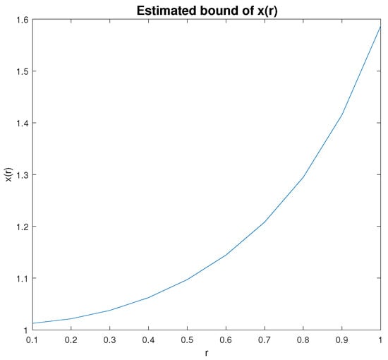
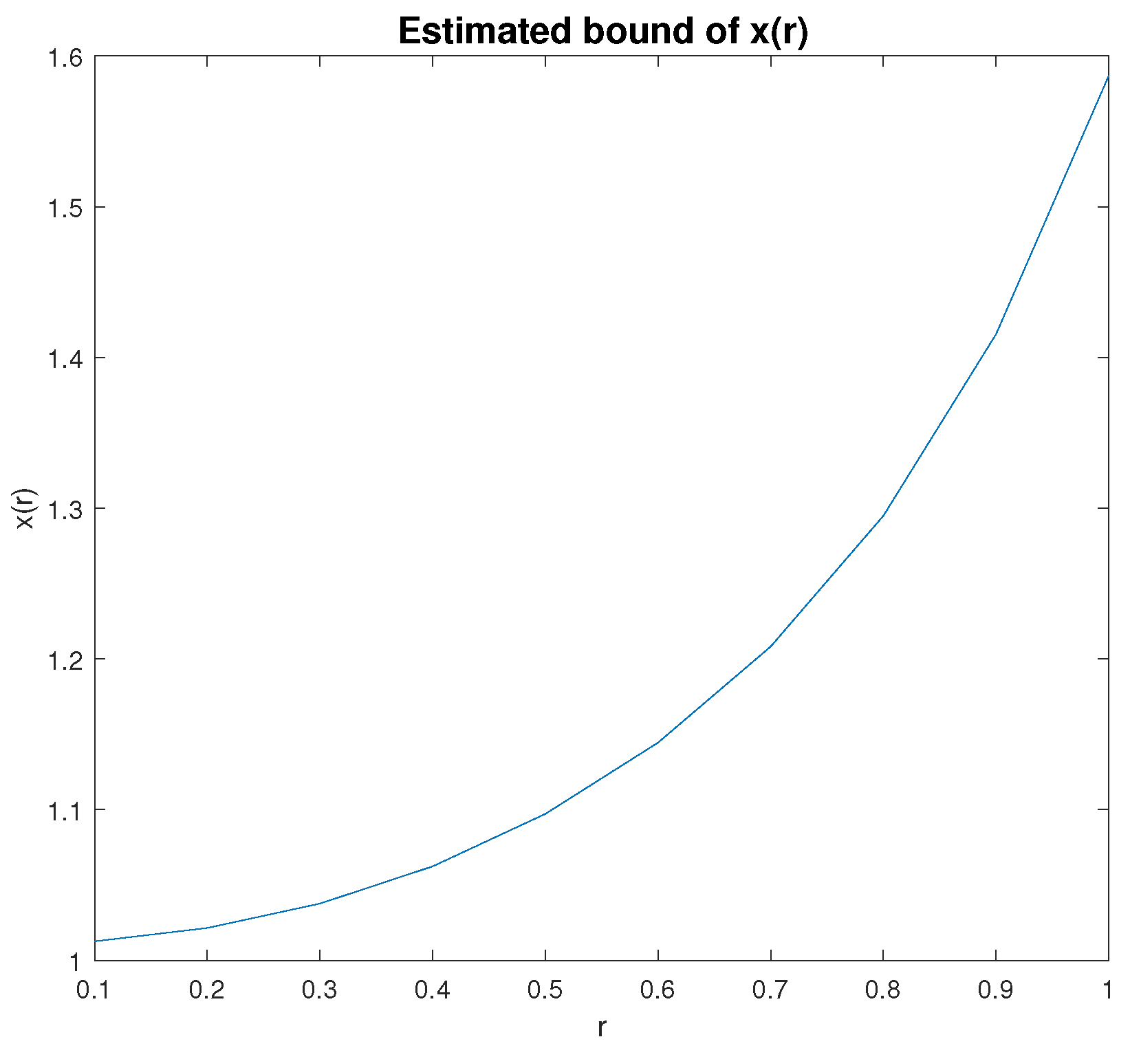
for all $r\in {\mathbb{R}}_{+}$, which gives boundedness and global existence for x, where Ψ and k are defined in Theorem 2 and

$$\begin{array}{c}\hfill \beta \left(r\right)=\frac{\mathtt{exp}\left(\underset{0}{\overset{\vartheta \left(r\right)}{\int }}\frac{\left(kp\left(\mu \right)+k(1-m)+\frac{1}{m}b\left(\mu \right)\right)}{{\vartheta }^{\prime }\left({\vartheta }^{-1}\left(\mu \right)\right)}d\mu \right)}{m{\phi }^{-1}\left(q\left(0\right)\right)-k\underset{0}{\overset{\vartheta \left(r\right)}{\int }}\frac{(m{q}^{\prime }\left({\vartheta }^{-1}\left(\mu \right)\right)+h\left(\mu \right))}{{\vartheta }^{\prime }\left({\vartheta }^{-1}\left(\mu \right)\right)}\mathtt{exp}\left(\underset{0}{\overset{\mu }{\int }}\left(kp\left(\theta \right)+k(1-m)+\frac{1}{m}b\left(\theta \right)\right)d\theta \right)d\mu },\end{array}$$

for all $r\in {\mathbb{R}}_{+}$. The estimated boundedness and existence of unknown x for $0\le r\le 1$ are shown in Figure 1.

Figure 1. Estimated boundedness and existence of $x\left(r\right)$.

At the end of this section, we present another example to demonstrate the result of Theorem 3.

Example 2. 

Consider the nonlinear differential equation of the initial value problem

$$\begin{array}{c}\hfill \left\{\begin{array}{c}{x}^{\prime }\left(r\right)=q^{\prime }\left(r\right)+F(r,x\left(\vartheta \left(r\right)\right)+H(r,x\left(\vartheta \left(t\right)\right),G(r,x\left(\vartheta \left(r\right)\right))),\forall r\in {\mathbb{R}}_{+},\hfill \\ x\left(0\right)=q\left(0\right),\hfill \end{array}\right.\end{array}$$

(57)

where $F,G\in \mathbb{E}({\mathbb{R}}_{+}^2,\mathbb{R})$, $H\in \mathbb{E}({\mathbb{R}}_{+}^3,\mathbb{R})$, and $q\left(0\right)$ is a positive constant. Assume that

$$\begin{array}{c}\hfill |q^{\prime }\left(r\right)+F(r,x\left(\vartheta \left(r\right)\right))|\le h^2\left(\vartheta \left(r\right)\right){\left|\phi \left(x\left(\vartheta \left(r\right)\right)\right)\right|}^2,\end{array}$$

(58)

$$\begin{array}{c}\hfill \left|G\right(r,x\left(\vartheta \right(r\left)\right)\left)\right|\le h\left(\vartheta \right(r\left)\right)\left|\phi \right(x\left(\vartheta \right(r\left)\right)\left)\right|,\end{array}$$

(59)

$$\begin{array}{c}\hfill \left|H\right(r,x,G|\le {\left|G\right|\left(\phi \right|x\left|\right)}^m+2\underset{0}{\overset{r}{\int }}{\left|G\right|}^{m}d\mu ,\end{array}$$

(60)

for all $r\in {\mathbb{R}}_{+},$ where $x,h,q,\vartheta ,\phi ,{\phi }^{\prime },k$, and m are already defined as in Theorem 3. Taking integration from 0 to r on (57), we have

$$\begin{array}{c}\hfill x\left(r\right)=q\left(r\right)+\underset{0}{\overset{r}{\int }}F(\mu ,x\left(\vartheta \left(\mu \right)\right))d\mu +\underset{0}{\overset{r}{\int }}H(\mu ,x\left(\vartheta \left(\mu \right)\right),G(\mu ,x\left(\vartheta \left(\mu \right)\right)))d\mu ,\forall r\in {\mathbb{R}}_{+}.\end{array}$$

(61)

Using (58)–(60) in (61), we obtain

$$\begin{array}{ccc}\hfill \left|x\right(r\left)\right|& =& \left|q\left(r\right)\right|+\underset{0}{\overset{r}{\int }}{h}^2{\left(\vartheta \left(\mu \right)\right)\left|\phi \left(x\left(\vartheta \left(\mu \right)\right)\right)\right|}^{2}d\mu +\underset{0}{\overset{r}{\int }}h\left(\vartheta \left(\mu \right)\right)\left|\phi \left(x\left(\vartheta \left(r\right)\right)\right)\right|\left(\right|\phi \left(x\left(\vartheta \left(\mu \right)\right)\right)|\hfill \\ & & +2\underset{0}{\overset{\mu }{\int }}h\left(\vartheta \left(\theta \right)\right)|\phi \left(x\left(\vartheta \left(\theta \right)\right)\right)d\theta {)}^{m}d\mu \hfill \\ & \le & \left|q\left(r\right)\right|+{\left(\underset{0}{\overset{\vartheta \left(r\right)}{\int }}\frac{h\left(\mu \right)\left|\phi \right(x\left(\mu \right)\left)\right|}{{\vartheta }^{\prime }\left({\vartheta }^{-1}\left(\mu \right)\right)}d\mu \right)}^2+\underset{0}{\overset{\vartheta \left(r\right)}{\int }}\frac{h\left(\mu \right)\left|\phi \right(x\left(\mu \right)\left)\right|}{{\vartheta }^{\prime }\left({\vartheta }^{-1}\left(\mu \right)\right)}(\phi \left(\right|x\left(\vartheta \left(\mu \right)\right)\left|\right)\hfill \\ & & +2\underset{0}{\overset{\mu }{\int }}h\left(\theta \right)\left|\phi \left(x\left(\theta \right)\right)\right|d\theta {)}^{m}d\mu ,\forall r\in {\mathbb{R}}_{+}.\hfill \end{array}$$

(62)

As an application of Theorem 3, the inequality (62) implies

$$\begin{array}{c}\hfill x\left(r\right)\le {\mathrm{\Psi }}^{-1}\left(\mathrm{\Psi }\left(q\left(0\right)\right)+\underset{0}{\overset{\vartheta \left(r\right)}{\int }}\frac{1}{{\vartheta }^{\prime }\left({\vartheta }^{-1}\left(\mu \right)\right)}\left(q^{\prime }({\vartheta }^{-1}\left(\mu \right)+h\left(\mu \right){\beta }_1\left(\mu \right)\right)d\mu \right),\forall r\in {\mathbb{R}}_{+},\end{array}$$

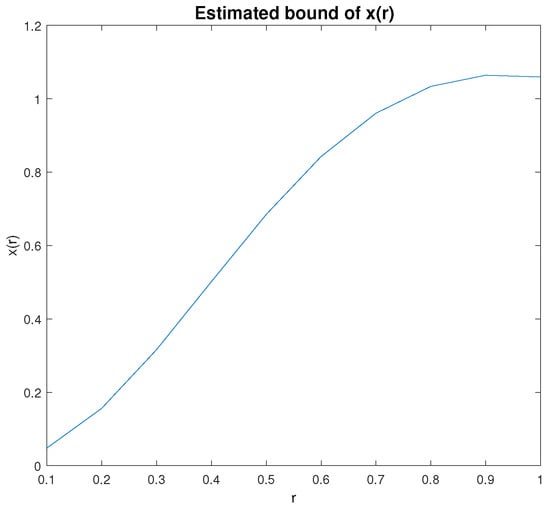
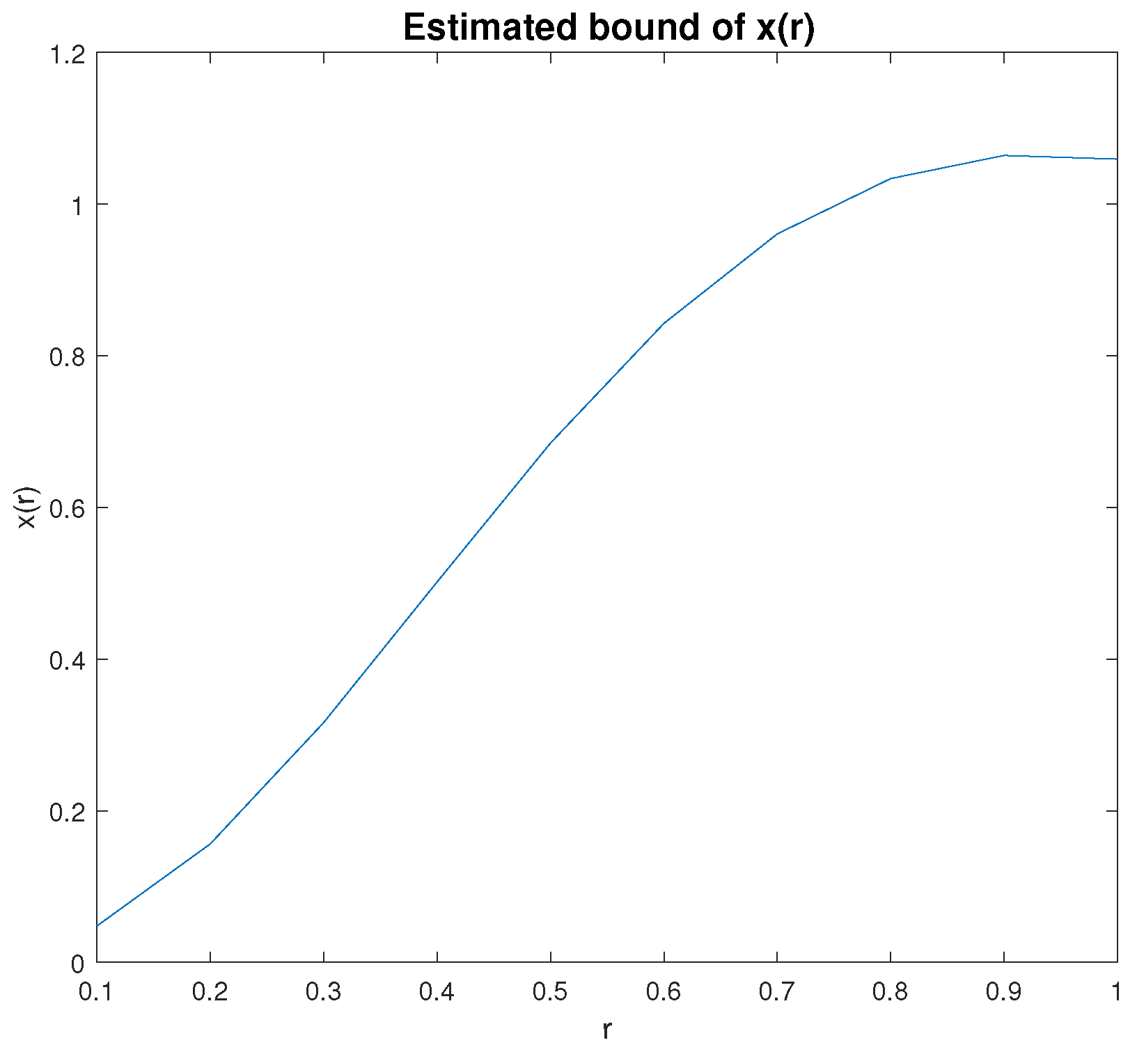
which gives boundedness and global existence for x, where Ψ and k are defined in Theorem 3 and

$$\begin{array}{c}\hfill {\beta }_1\left(r\right)=\frac{\mathtt{exp}\left(2(1+\frac{1}{m})\underset{0}{\overset{\vartheta \left(r\right)}{\int }}\frac{h\left(\mu \right)}{{\vartheta }^{\prime }\left({\vartheta }^{-1}\left(\mu \right)\right)}d\mu \right)}{{\left(m\phi \left(q\right(0\left)\right)+1-m\right)}^{-1}-k\underset{0}{\overset{\vartheta \left(r\right)}{\int }}\frac{m{q}^{\prime }\left({\vartheta }^{-1}\left(\mu \right)\right)+h\left(\mu \right)}{{\vartheta }^{\prime }\left({\vartheta }^{-1}\left(\mu \right)\right)}\mathtt{exp}\left(2(1+\frac{1}{m})\underset{0}{\overset{\mu }{\int }}h\left(\theta \right)d\theta \right)d\mu },\end{array}$$

for all $r\in {\mathbb{R}}_{+}$. The estimated boundedness and existence of unknown x for $0\le r\le 1$ are shown in Figure 2.

Figure 2. Estimated boundedness and existence of $x\left(r\right)$.

5. Conclusions

It is well known that there exists a class of mathematical models that are described by differential equations, and a large number of differential equations do not possess exact solutions or the existence of solutions or the boundedness of solutions. On the other hand, integral inequalities occupy a very privileged position in all mathematical sciences, and they have many applications to questions of existence, stability, boundedness, and uniqueness, and to the asymptotic behavior of the solutions of nonlinear integro-differential equations (see [1,2,3,4]). But, in certain cases, the existence and boundedness studied by the integral inequalities given in the current literature (see references) are not directly applicable, and they are not feasible for studying the stability and asymptotic behavior of the solutions of classes of more general nonlinear retarded integral, differential, and integro-differential equations. However, the inequalities established in this manuscript permit us to analyze the existence, uniqueness, stability, boundedness, and asymptotic behavior, as well as the other properties of the solutions of classes of more general retarded nonlinear differential, integro-differential, and integral equations. Many renowned and existing famous inequalities can be explored on the basis of different choices of parameters (see Remarks 1–4) from the integral inequalities of this article. The importance of these inequalities stems from the fact that it is applicable in certain situations in which other available inequalities do not apply directly. As such, these inequalities can handle the problems of nonlinear partial differential equations in applied sciences. This research work will ensure the opening up of new opportunities for the studying of nonlinear dynamic inequalities on a time-scale structure of a varying nature.

References

- Bainov, D.; Simeonov, P. Integral Inequalities and Applications; Kluwer Academic: Dordrecht, The Netherlands, 1992. [Google Scholar]
- Hardy, G.H.; Littlewood, J.E.; Polya, G. Inequalities, 2nd ed.; Cambridge University Press: Cambridge, UK, 1952. [Google Scholar]
- Pachpatte, B.G. Inequalities for Differential and Integral Equations; Academic Press: London, UK, 1998. [Google Scholar]
- Boichuk, A.A.; Samoilenko, A.M. Generalized Inverse Operators and Fredholm Boundary Value Problems, 2nd ed.; Walter de Gruyter: Berlin, Germany; Boston, MA, USA, 2016. [Google Scholar]
- Shakoor, A.; Samar, M.; Athar, T.; Saddique, M. Results on retarded nonlinear integral inequalities with mix powers and their applications in delay integro-differential. Ukr. Math. J. 2023, 75, 478–493. [Google Scholar] [CrossRef]
- Sun, Y.; Xu, R. Some weakly singular Volterra integral inequalities with maxima in two variables. J. Inequal. Appl. 2023, 2023, 36. [Google Scholar] [CrossRef]
- Abuelela, W.; El-Deeb, A.A.; Baleanu, D. On Some Generalizations of Integral Inequalities in n Independent Variables and Their Applications. Symmetry 2022, 14, 2257. [Google Scholar] [CrossRef]
- Gronwall, T.H. Note on the derivatives with respect to a parameter of the solutions of a system of differential equations. Ann. Math. 1919, 20, 292–296. [Google Scholar] [CrossRef]
- Bellman, R. The stability of solutions of linear differential equations. Duke Math. J. 1943, 10, 643–647. [Google Scholar] [CrossRef]
- Jiang, F.; Meng, F. Explicit bounds on some new nonlinear integral inequalities with delay. J. Comput. Appl. Math. 2007, 205, 479–486. [Google Scholar] [CrossRef]
- Agarwal, R.P.; Deng, S.; Zheng, W. Generalization of a retarded Gronwall-like inequality and its applications. Appl. Math. Comput. 2005, 165, 599–612. [Google Scholar] [CrossRef]
- Abdeldaim, A.; El-Deeb, A.A. On generalized of certain retarded nonlinear integral inequalities and its applications in retarded integro-differential equations. Appl. Math. Comput. 2015, 256, 375–380. [Google Scholar] [CrossRef]
- Pachpatte, B.G. A note on Gronwall-Bellman inequality. Math. Anal. Appl. 1973, 44, 758–762. [Google Scholar] [CrossRef]
- Abdeldaim, A.; El-Deeb, A.A. On some generalizations of certain retarded nonlinear integral inequalities with iterated integrals and an application in retarded differential equation. J. Egypt. Math. Soc. 2015, 23, 470–475. [Google Scholar] [CrossRef]
- Wang, W.S. Some retarded nonlinear integral inequalities and their applications in retarded differential equations. J. Inequal. Appl. 2012, 2012, 75. [Google Scholar] [CrossRef]
- Abdeldaim, A.; Yakout, M. On some new integral inequalities of Gronwall-Bellman-Pachpatte type. Appl. Math. Comput. 2011, 217, 7887–7899. [Google Scholar] [CrossRef]
- Shakoor, A.; Ali, I.; Azam, M.; Rehman, A.; Iqbal, M.Z. Further Nonlinear Retarded Integral Inequalities for Gronwall-Bellman Type and Their Applications. Iran. J. Sci. Technol. Trans. Sci. 2019, 43, 2559–2568. [Google Scholar] [CrossRef]
- Cheung, W.S. Some new nonlinear inequalities and applications to boundary value problems. Nonlinear Anal. 2006, 64, 2112–2128. [Google Scholar] [CrossRef]
- Shakoor, A.; Ali, I.; Wali, S.; Rehman, A. Some Generalizations of Retarded Nonlinear Integral Inequalities and Its Applications. J. Math. Inequal. 2020, 14, 1223–1235. [Google Scholar] [CrossRef]
- Shakoor, A.; Samar, M.; Wali, S.; Saleem, M. Retarded nonlinear integral inequalities of Gronwall-Bellman-Pachpatte type and their applications. Honam Math. J. 2023, 45, 54–70. [Google Scholar]
Disclaimer/Publisher’s Note: The statements, opinions and data contained in all publications are solely those of the individual author(s) and contributor(s) and not of MDPI and/or the editor(s). MDPI and/or the editor(s) disclaim responsibility for any injury to people or property resulting from any ideas, methods, instructions or products referred to in the content. |
© 2024 by the authors. Licensee MDPI, Basel, Switzerland. This article is an open access article distributed under the terms and conditions of the Creative Commons Attribution (CC BY) license (https://creativecommons.org/licenses/by/4.0/).