Mathematical Model of the Evolution of a Simple Dynamic System with Dry Friction

Abstract

A simple dynamic system with dry friction is studied theoretically and numerically. Models of systems including dry friction are not easily obtained, as defining the relationship between the friction force and the relative velocity presents a significant challenge. It is known that friction forces exhibit notable discontinuities when there is a change in the direction of motion. Additionally, when the relative motion ceases, the friction force can assume any value within a certain range. In the literature, numerous models of dry friction are presented, and most of them assume a biunivocal dependency of the friction force with respect to relative velocity. The dynamic system considered here is a tilted rod with spherical ends, initially at rest. Dry friction forces are evident at the contact point with the horizontal plane. The ball–plane contact highlights the rolling friction or/and sliding friction. The problem is theoretically solved after adopting one of the two cases of friction: rolling friction or sliding friction. The nonlinear differential equations of motion have been derived, along with expressions for the magnitude of the normal reaction and the friction force. The results of the model are displayed graphically for three different sets of values for the coefficient of friction. It is revealed that there is a critical value of the coefficient of friction that determines the transition from rolling to sliding regimes. To validate the theoretical model, dynamic simulation software was utilised. The excellent match between the theoretical predictions and the results from the numerical simulation confirms the accuracy of the proposed analytical solution.

1. Introduction

When two solid bodies bounded by nonconforming surfaces, labelled Σ₁ and Σ₂ in Figure 1, come into contact, they interact in a simple and general way by forming two regions of extremely small dimensions that become common between them. Under the hypothesis that the two bodies are slightly deformable, in the limit, the rigid body assumption can be accepted and thus the two bodies will have in common the points $C_1$ and $C_2$. The common contact points are well defined by the common normal $\mathit{n}$ and the common tangent plane $\left(P\right)$. The relative motion between the two bodies is completely defined by the relative velocity ${\mathit{v}}_{C_2{C}_1}$ between the overlapping points in contact and the relative angular velocity ${\mathit{\omega }}_{21}$ (denoted $\mathit{\omega }$). It should be noted that while the angular velocity can have an arbitrary direction, it includes a component ${\mathit{\omega }}_s$ parallel to the normal $\mathit{n}$, characterising the spin motion, and a second component ${\mathit{\omega }}_r$ located in the tangent plane, which defines the rolling motion. Meanwhile, the relative velocity $\mathit{v}$ is contained in the tangent plane. The axiom of constraints enables the substitution of the support, which requires the two bodies to always have a point of contact, with a normal reaction force $\mathit{N}$ which blocks the relative motion in the normal direction. The torsor of the friction forces opposes the relative motion between the two bodies by its components: $\mathit{T}$ is the friction force parallel and of opposite direction to the linear velocity $\mathit{v}$; ${\mathit{M}}_s$ is the spin friction torque, parallel and of opposite direction to the angular spin velocity ${\mathit{\omega }}_s$; and ${\mathit{M}}_r$ is the rolling friction torque parallel and of opposite direction to the angular velocity ${\mathit{\omega }}_r$. To solve the dynamics problem, the dependencies of the three components of the friction torsor must be specified as functions of the normal reaction, of the relative motion from the contact point, and of the presence/absence of lubricant film between the two surfaces.

In the case of lubricated contact, when a continuous and sufficient film of lubricant maintains the two surfaces apart, friction occurs only within the fluid film. According to Newton [1], the total friction force is proportional to the relative velocity:

$$\mathit{T}=-cv{\mathit{i}}_v=-cv(\mathit{v}/v)$$

(1)

Equation (1) is valid as long as

$$v\le 50 \mathrm{m}/\mathrm{s}$$

(2)

For velocity values greater than this, the following dependency is considered [2]:

$$\mathit{T}=-c{v}^2{\mathit{i}}_v=-c{v}^2\frac{\mathit{v}}{v}$$

(3)

In the case of dry friction, the first quantitative relationship was presented by Coulomb [3] in 1785. According to this equation, the dry friction force is proportional to the normal force N:

$$\mathit{T}=-\mu N\frac{\mathit{v}}{v}$$

(4)

It can be noted that Equation (4) is valid as long as relative motion exists, $v\ne 0$. Experimentally, it has been observed that the immobile state is maintained if the external tangential forces do not exceed the extreme values of the friction force as expressed by Equation (4). The Coulomb model for the dry friction force is presented in Figure 2.

The model in Figure 2 has two main drawbacks, concerning the origin point: the friction force takes multiple values and an ordinate discontinuity occurs. These two aspects can lead to instability in the numerical analysis processes. In order to avoid this inconvenience, the function in Figure 2 was approximated with continuous functions. Marques [4] cites authors [5,6,7] who propose various approximations for the Coulomb friction force related to velocity (Figure 3).

A basic experiment reveals that when a force which increases in time is applied to an immobile body, at a given instant, the body starts moving. By maintaining the force at this maximum value, it is noted that the motion of the body is not uniform, as the models in Figure 2 and Figure 3 claim, but accelerated. The conclusion is reached that, after the initiation of motion, the friction force is smaller than the maximum force from the static case. In this instance, the friction force is characterised using two coefficients of friction: the coefficient of static friction ${\mu }_{st}$ and the coefficient of dynamic friction ${\mu }_d$, and it is expressed using the following relation:

$$\left\{\begin{array}{c}\left|T\right|={\mu }_{d}N if v\ne 0\\ \left|T\right|\le {\mu }_{st}N if v=0\end{array}\right.$$

(5)

The graphical representation of the dry friction force, Equation (5), is given in Figure 4.

A more general case occurs when, between the two surfaces, a fluid film is interposed, which is disrupted when the relative motion between the contacting points is cancelled, known as the Stribeck effect [8] (Figure 5). Figure 6 shows approximations of the models from Figure 5, where multiple values at the origin are avoided.

Due to the need for a more accurate description of the dynamic behaviour of systems with friction, more complex friction models have been developed. Because the data concerning the current state of the system were insufficient, other variables considering the history of loading were introduced [9,10] for obtaining the models.

An example is the Dahl model [11,12] that was developed to describe the dynamic behaviour of the ball bearings. The contact is modelled as the interaction between the bristles attached to the surfaces (bristle analogy), as represented in Figure 7, capable of describing the pre-sliding phenomenon.

According to the Dahl model [11,12], the friction force is expressed as

$$T={\sigma }_{0}z$$

(6)

where

$$\frac{dz}{dt}=\left[1-\frac{{\sigma }_0}{F_C}z\mathrm{sgn}(v)\right]v$$

(7)

and $F_C$ is the Coulomb dynamic friction force and ${\sigma }_0$ characterises the stiffness of the bristle. The newly defined variable $z$ helps highlight the pre-sliding phenomenon and eliminates the force discontinuity at the origin. The Dahl model initiated a series of friction models that progressively increase in complexity with the aim of incorporating as many parameters characteristic of the friction phenomenon as possible.

Another model widely used is the LuGre model [13,14,15], with the friction force being described by the following relation [13]:

$$\frac{dz}{dt}=\left[1-\frac{{\sigma }_0}{G\left(v\right)}z\mathrm{sgn}(v)\right]v$$

(8)

$$T={\sigma }_{0}z+{\sigma }_1\frac{dz}{dt}+{\sigma }_{2}v$$

(9)

where ${\sigma }_1$ is the damping coefficient of the bristle, ${\sigma }_2$ is the viscous friction coefficient, and $G\left(v\right)$ is a function that describes the Stribeck effect by the following relation:

$$G\left(v\right)=F_C+(F_S-F_C)\exp [-(v/v_S{)}^{{\delta }_0}]$$

(10)

where $v_s$ is a parameter indicating how quickly the function $G\left(v\right)$ approaches $F_C$, and ${\delta }_0$ is an exponent [16,17,18] that takes values in the range [0.5…2].

A concrete example of dry friction types in systems can be seen in recent research that applies to the flow of lava on an inclined surface, modelled as a stick-slip effect [19,20]. The mathematical approach used involves fractional derivatives, which allow for a generalisation of the stick-slip model.

This paper presents a short review of dry friction models, starting with the simple Coulomb model and then continuing with models with increasing complexity such as Stribeck, Dahl, and LuGre.

The dynamic model proposed for study is a simple system consisting of a rod that has spheres attached to its ends, with one sphere being brought into contact with a horizontal plane. The system is allowed to move freely under the action of its own gravity. Dry friction is considered between the ball and the horizontal plane. We assume a friction model characterised by a static friction coefficient and dynamic friction coefficient. For the studied dynamic system, the theories of rigid dynamics are applied and the equations of motion and the expression of reaction forces are obtained, for the cases of pure rolling and sliding motion. The equations of motion are numerically integrated and, after that, the kinematic parameters and the reaction forces from contact are represented versus time.

The simulation with dynamic analysis software shows that the motion of the system is strongly influenced by the size of the friction forces in the ball–plane contact. It should be noted that the simulation software uses, in the ball–plane contact, a continuous dependence of the friction coefficient on the relative velocity. For the ball–plane friction, the model is adopted in which the coefficient of friction has different values, depending on the zero or non-zero value of the relative speed, being characterised by two values: the coefficient of static friction ${\mu }_{st}$ and the coefficient of dynamic friction ${\mu }_d$. Although the model is extremely simple, the existence of time intervals in which the relative velocity is zero in the ball–plane contact substantially complicates the dynamic study, as Pennestri [21] shows: “In kinematic pairs with no relative motion the computation of friction forces is not straightforward”. This dependence was chosen because the adoption of other, more complex models (for example, the Dahl model and LuGre model) that would better describe the dependence of the friction force on the relative velocity would have as their main disadvantage the presence of some parameters whose values are very difficult to specify. For the Dahl model, for example, it is necessary to specify the values of two parameters about which Pennestri stated that “The authors could not find a table relating the Coulomb friction coefficients with Dahl friction parameters” [21], and that the values of the two parameters were achieved through experiments. In the case of the more complex LuGre model, the number of parameters required to be predicted is six [4], with the task of identifying their values thus being even more difficult. The adoption of the friction coefficient model with discontinuity at the origin allowed the modelling of the proposed system by the presence of sliding or pure rolling, depending on the presence or absence of the relative velocity in contact. It should be noted that the results of the discontinuous friction coefficient modelling, proposed by the authors, are in full agreement with the results obtained with the simulation software.

The conclusions of this paper are presented in the final section.

2. Materials and Methods

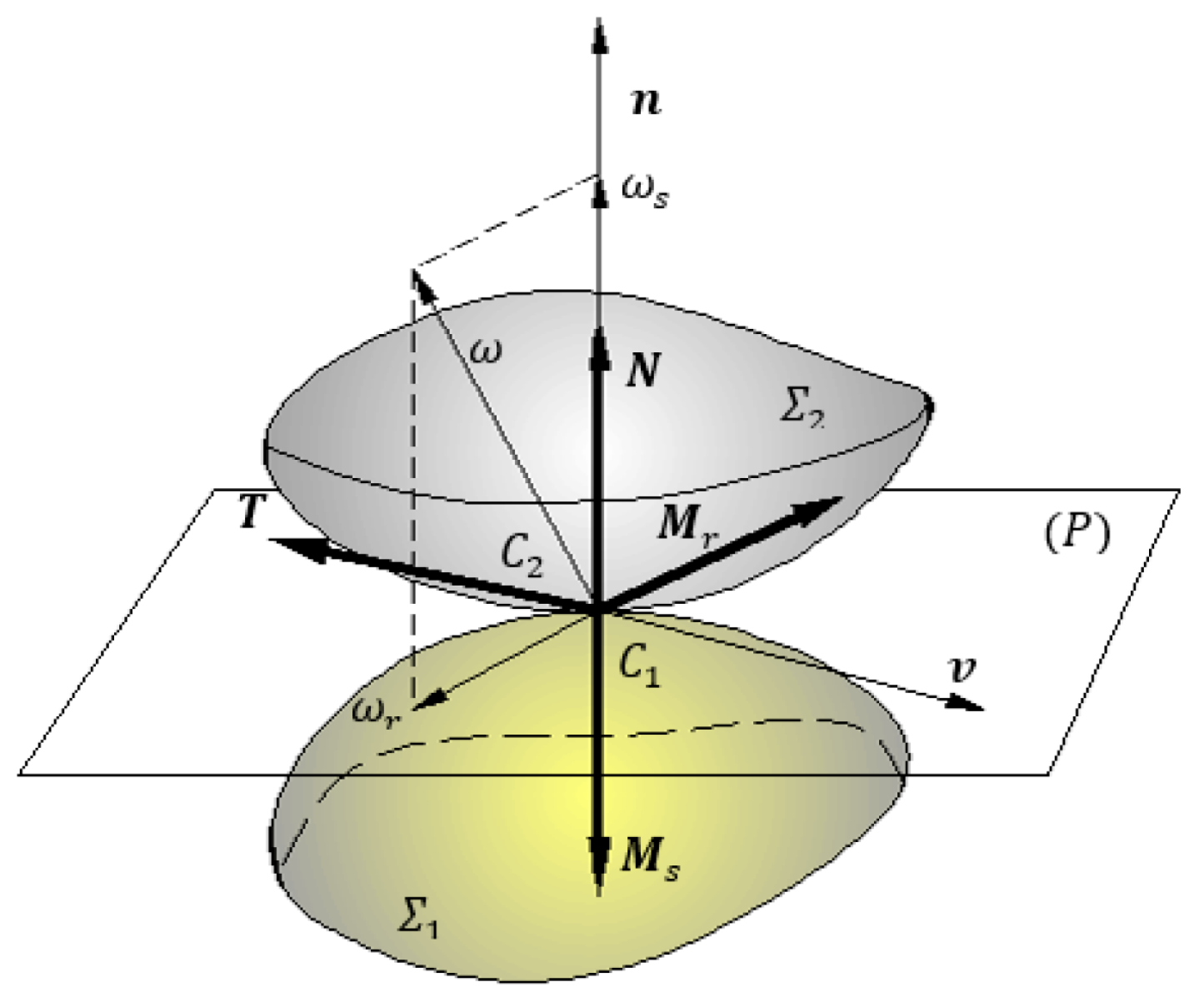
2.1. The Equations of the Dynamic Model

The dynamic system to be analysed is presented in Figure 8. An axial symmetric body has at one end a sphere of radius $r$ that is supported by a horizontal plane with friction.

The centre of mass denoted $\Gamma$ is positioned on the axis of symmetry at a distance $\xi$ from the centre of the sphere. The body has mass $M$ and moment of inertia $J_{\Gamma }$ with respect to an axis passing through centre of mass $\Gamma$ and normal to the plane of motion. The adopted friction model is presented in Figure 4, considering dynamic and static friction, characterised by the coefficients of friction ${\mu }_d$ and ${\mu }_s$, respectively. At the initial moment, the body is motionless, and the direction of its axis makes the angle ${\theta }_o$ with the horizontal direction.

In order to solve the problem, two Cartesian systems are attached. One is fixed, $xyz$, with the versors $\mathit{i}$, $\mathit{j}$, $\mathit{k}$:

$$\mathit{i}=\left[\begin{array}{c}1\\ 0\\ 0\end{array}\right], \mathit{j}=\left[\begin{array}{c}0\\ 1\\ 0\end{array}\right], \mathit{k}=\left[\begin{array}{c}0\\ 0\\ 1\end{array}\right].$$

(11)

The other is a mobile frame, $x^{\prime }{y}^{\prime }{z}^{\prime }$, attached to the body, with the origin $O$ in the centre of the ball. It is accepted, without reducing the generality of the problem, that the $O{x}^{\prime }$ axis passes both through the centre of the ball $O$ and the centre of mass of the body $\Gamma$. The $O{z}^{\prime }$ axis of the mobile system coincides with the $Oz$ axis of the fixed frame and the axis $O{y}^{\prime }$ completes the right cartesian frame. The position and the orientation of the axes of the mobile frame are stipulated by the abscissa $x_O$ of the point $O$ and by the oriented angle $\theta$ between the $O{x}^{\prime }$ axis and the $\mathit{i}$ versor. It results in the following:

$${\mathit{i}}^{\prime }=\left[\begin{array}{c}\cos \theta \\ \sin \theta \\ 0\end{array}\right], {\mathit{j}}^{\prime }=\left[\begin{array}{c}-\sin \theta \\ \cos \theta \\ 0\end{array}\right], {\mathit{k}}^{\prime }=\mathit{k}$$

(12)

The external forces acting upon the body are the weight G applied in the centre of mass $\Gamma$:

$$\mathit{G}=\left[\begin{array}{c}0\\ -Mg\\ 0\end{array}\right]$$

(13)

and the reactions applied at the contact point: the normal reaction $\mathit{N}$ and the tangential reactions (friction force) $\mathit{T}$:

$$\mathit{N}=N\mathit{j}=\left[\begin{array}{c}0\\ N\\ 0\end{array}\right]$$

(14)

$$\mathit{T}=T\mathit{i}=\left[\begin{array}{c}T\\ 0\\ 0\end{array}\right]$$

(15)

It is apparent that all the forces acting upon the body are contained in the $xy$ plane; therefore, the motion of the body is plane-parallel and the body has three degrees of freedom: translational motions in the $xy$ plane and rotation about the $z$ axis. The analysis of the body’s motion involves applying the linear momentum theory, specifically in the form of the theory of motion of the centre of mass, and the theory of angular momentum concerning the centre of mass. Based on Figure 8, the position vector of the centre of mass is expressed in the form:

$${\mathit{r}}_{\Gamma }=x_O\mathit{i}+r\mathit{j}+\xi {\mathit{i}}^{\prime }=\left[\begin{array}{c}{x}_O\\ 0\\ 0\end{array}\right]+\left[\begin{array}{c}0\\ r\\ 0\end{array}\right]+\left[\begin{array}{c}\xi \cos \theta \\ \xi \sin \theta \\ 0\end{array}\right]$$

(16)

Relation (16) permits finding the trajectory of the centre of mass with respect to the fixed frame:

$$\left\{\begin{array}{c}{x}_{\Gamma }\left(t\right)=x_O+\xi \cos \theta \\ y_{\Gamma }\left(t\right)=r+\xi \sin \theta \end{array}\right.$$

(17)

The relations (17) are differentiated with respect to time twice:

$$\left\{\begin{array}{c}{a}_{\Gamma x}={\ddot{x}}_O-\xi {\dot{\theta }}^2\cos \theta -\xi \ddot{\theta }\sin \theta \\ a_{\Gamma y}=-\xi {\dot{\theta }}^2\sin \theta +\xi \ddot{\theta }\cos \theta \end{array}\right.$$

(18)

Considering relations (13)–(15) and (18), the equation of motion of the centre of mass is as follows:

$$M{\mathit{a}}_{\Gamma }=\mathit{G}+\mathit{N}+\mathit{T}$$

(19)

This leads to the following two scalar equations:

$$\left\{\begin{array}{l}M({\ddot{x}}_O-\xi {\dot{\theta }}^2\cos \theta -\xi \ddot{\theta }\sin \theta )=T\\ M(-\xi {\dot{\theta }}^2\sin \theta +\xi \ddot{\theta }\cos \theta )=-Mg+N\end{array}\right.$$

(20)

The angular momentum theory is written with respect to the centre of mass $\Gamma$:

$$\left[\begin{array}{l}0\\ 0\\ J_{\Gamma }\ddot{\theta }\end{array}\right]=\overline{\Gamma C}\times (\mathit{N}+\mathit{T})$$

(21)

where

$$\overline{\Gamma C}=-\xi {\mathit{i}}^{\prime }-r\mathit{j}=\left[\begin{array}{c}-\xi \cos \theta \\ -r-\xi \sin \theta \\ 0\end{array}\right]$$

(22)

Equation (22) gives a single scalar equation:

$$J_{\Gamma }\ddot{\theta }=-N\xi \cos \theta +T\xi \sin \theta +Tr$$

(23)

Thus, the motion of the body is described by the following system of equations:

$$\left\{\begin{array}{l}M({\ddot{x}}_O-\xi {\dot{\theta }}^2\cos \theta -\xi \ddot{\theta }\sin \theta )=T\\ M(-\xi {\dot{\theta }}^2\sin \theta +\xi \ddot{\theta }\cos \theta )=-Mg+N\\ J_{\Gamma }\ddot{\theta }=-N\xi \cos \theta +T\xi \sin \theta +Tr\end{array}\right.$$

(24)

2.2. The Solutions of the System of Equations of Motion

The unknowns of the system (24) are the kinematic position parameters $x_O$ and $\theta$ and the components $N$ and $T$ of the reaction from the contact point. With four unknowns and three equations, the system is undetermined, and an additional equation is required. For this purpose, the two types of motion that can occur at the contact point are considered:

Pure rolling motion, characterised by the simultaneous conditions:

$${\mathit{v}}_{C{C}_0}=0$$

(25)

$$\left|\frac{T}{N}\right|<{\mu }_s$$

(26)

Sliding motion, that arises when at least one of the conditions (25) or (26) is not satisfied.

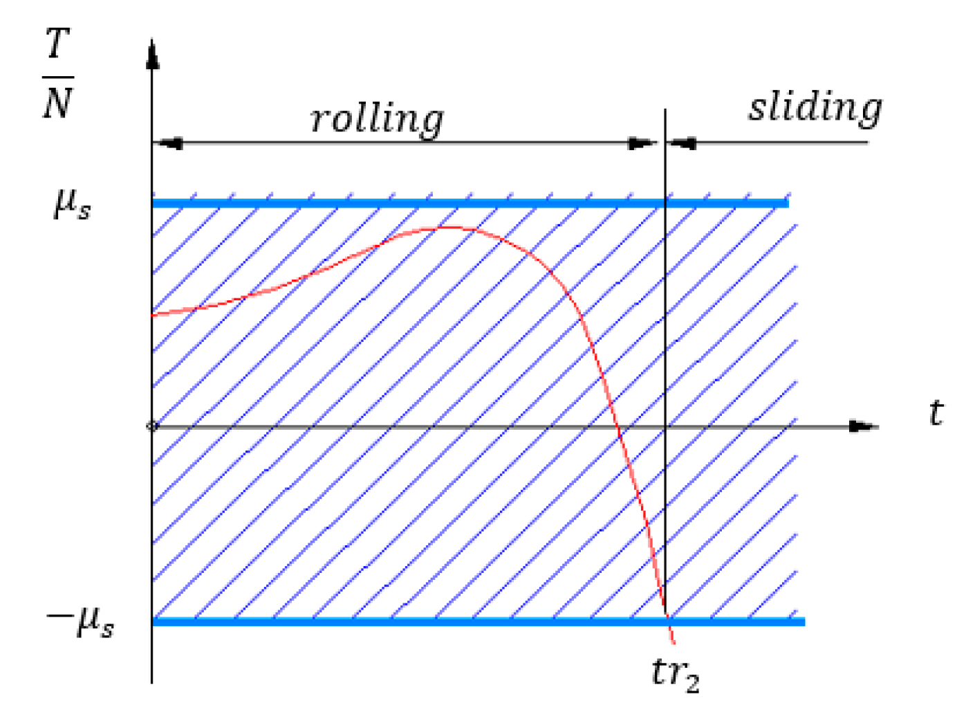
2.2.1. The Study of the Motion under Pure Rolling Hypothesis

We first study the pure rolling motion because condition (25) is always satisfied at the initial moment when the body is launched from the resting state. To apply relation (25), the expression of the relative velocity at the point of contact is necessary:

$${\mathit{v}}_{C_0}=\mathbf{0}$$

(27)

And the velocity of point $C$ from the mobile body is found using Euler’s formula:

$${\mathit{v}}_C={\mathit{v}}_O+\mathit{\omega }\times \overline{OC}={\dot{x}}_O\mathit{i}+\dot{\theta }\mathit{k}\times (-r\mathit{j})=({\dot{x}}_O+\dot{\theta }r)\mathit{i}$$

(28)

Condition (25) has as a consequence the following relation:

$${\dot{x}}_0=-\dot{\theta }r$$

(29)

The derivative of relation (29) gives

$${\ddot{x}}_0=-\ddot{\theta }r$$

(30)

Equation (29) is integrated with respect to time and considering the initial conditions:

$$\theta (0)={\theta }_0,\dot{\theta }(0)=0,$$

(31)

and it results in the following:

$$x_O=-\theta r+{\theta }_{0}r$$

(32)

By replacing Equation (30) by system (24), it results in a system of unknowns $\theta ,$ $N$, and $T$:

$$\ddot{\theta }=-\frac{\frac{g}{r}+{\dot{\theta }}^2}{1+\frac{J_{\Gamma }}{M{r}^2}+2\frac{\xi }{r}\sin \theta +{\left(\frac{\xi }{r}\right)}^2}\frac{\xi }{r}\cos \theta$$

(33)

$$T=-\left[\left(1+\frac{\xi }{r}\sin \theta \right)\ddot{\theta }+\frac{\xi }{r}{\dot{\theta }}^2\cos \theta \right]Mr$$

(34)

$$N=\left(\frac{\xi }{r}\ddot{\theta }\cos \theta -\frac{\xi }{r}{\dot{\theta }}^2\sin \theta +\frac{g}{r}\right)Mr$$

(35)

The body has a single degree of freedom, represented by the $\theta$ angle. The integration of the nonlinear equation, Equation (33), is necessary to obtain the variation in the angle $\theta$. In this case, the Runge–Kutta algorithm was used. With known $\theta$ variation, the variation in the normal reaction $N$ and of the friction force $T$ can be found. These are necessary to verify condition (26), which ensures pure rolling.

For the real cases, it was observed that the time variation in the curve of the ratio $T/N$ has a shape as presented in Figure 9. Three possible situations can occur, depending on the magnitude of the friction forces from the system (Figure 10, Figure 11 and Figure 12).

Figure 10 presents the case when the friction forces have small values. The moments when the ratio $T/N$ takes the values ${\mu }_s$ and $-{\mu }_s$, respectively, are denoted as $t{r}_1$ and $t{r}_2$. At the instant of launch, the body is motionless and condition (25) is satisfied. In the interval $[0,t{r}_1]$, the condition $T/N\le {\mu }_s$ is not satisfied; therefore, sliding motion exists. The same situation can be met for conformal dry contact, fixed-stick, followed by sliding [22]. In the interval $[t{r}_1,t{r}_2]$, the condition $|T/{\rm N}|\le {\mu }_s$ is satisfied, but at the moment $t{r}_1$, the body is in sliding motion and it is quite improbable that the kinematic parameters ${\mathit{v}}_O$ and $\omega$ satisfy condition (25). Therefore, during this interval, the sliding motion continues at the point of contact. After the moment ${tr}_2$, $T/N<-{\mu }_s$ and the sliding motion continues. In this case, sliding motion takes place in the entire domain.

Figure 11 shows the variation in the ratio $T/N$ for intermediate values of friction. At the initial moment, both conditions (relations (25) and (26)) are simultaneously satisfied and pure rolling exists at the contact point. The rolling motion takes place until the moment $t{r}_1$, defined here as the minimum values from the two solutions of the equation:

$$\left\{\begin{array}{l}T\left(t^{\prime }{r}_1\right)/N\left(t^{\prime }{r}_1\right)={\mu }_s\\ T\left(t^{″}{r}_1\right)/N\left(t^{″}{r}_1\right)={\mu }_s\end{array}\right.$$

(36)

$$t{r}_1=\min (t^{\prime }{r}_1,t^{″}{r}_2),$$

(37)

Beyond this point, as observed in the previous case, the motion continues with sliding.

Figure 12 illustrates the scenario where friction forces are significant. In this case, $\max (T/N)<{\mu }_s$ results in imaginary values of $t^{\prime }{r}_1$ and $t^{″}{r}_2$, and condition (26) is verified in the entire interval $[0,t{r}_2]$. Based on this observation, it can be stated that pure rolling occurs in the interval $[0,t{r}_2]$ and is followed by sliding motion thereafter.

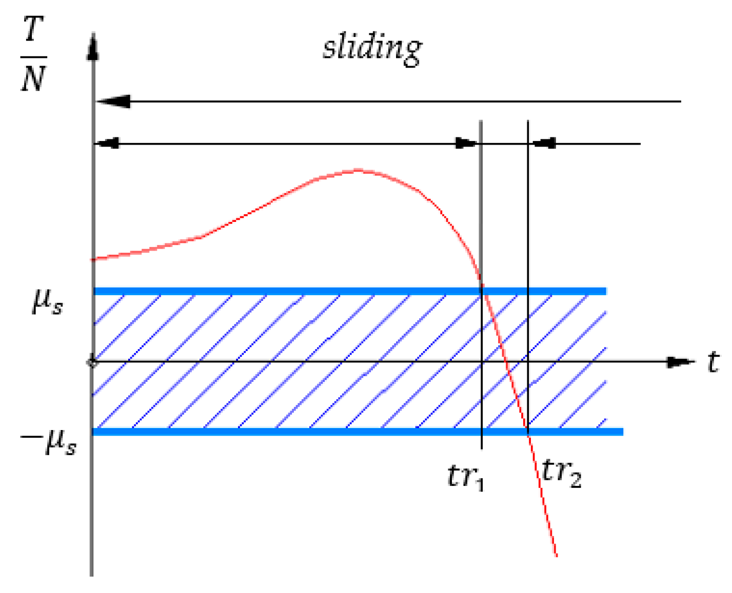
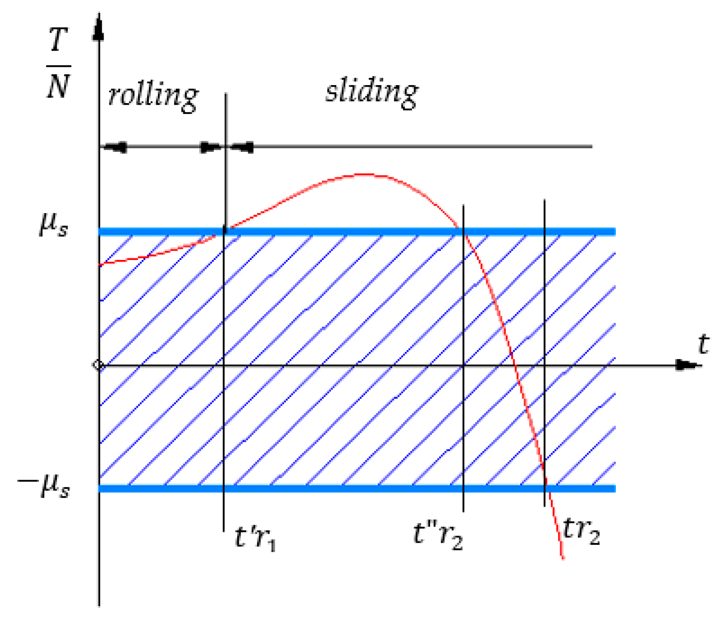
2.2.2. The Study of the Motion under Sliding Hypothesis

As shown above, regardless of the friction force values, there will always be an interval of time during the evolution of the system when the sliding motion exists. In this situation, the system will present two degrees of freedom represented by the rotation angle $\theta$ and the displacement $x_O$ of the centre of the ball. Thus, the friction force $\mathit{T}$ is not independent of the normal force but is expressed using the Amonton–Coulomb law:

$$T=-{\mu }_{d}N\mathrm{sgn}({\dot{x}}_0+\dot{\theta }r)$$

(38)

where ${\mu }_d$ represents the coefficient of dynamic friction and the function sgn is the signum function.

$$\mathrm{sgn}(x)=\left\{\begin{array}{cc}1,& \mathrm{i}\mathrm{f} x>0\\ 0,& \mathrm{i}\mathrm{f} x=0\\ -1,& \mathrm{i}\mathrm{f} x<0\end{array}\right.$$

(39)

By substituting expression (38) in system (24), a system of scalar equations is obtained:

$$\left\{\begin{array}{l}M({\ddot{x}}_O-\xi {\dot{\theta }}^2\cos \theta -\xi \ddot{\theta }\sin \theta )=-{\mu }_{d}N\mathrm{sgn}({\dot{x}}_0+\dot{\theta }r)\\ M(-\xi {\dot{\theta }}^2\sin \theta +\xi \ddot{\theta }\cos \theta )=-Mg+N\\ J_{\Gamma }\ddot{\theta }=-N\xi \cos \theta -{\mu }_{d}N\mathrm{sgn}({\dot{x}}_0+\dot{\theta }r\left)\right(\xi \sin \theta +r)\end{array}\right.$$

(40)

The solutions of system (24) are

$$N=\frac{\left(\frac{g}{r}-\frac{\xi }{r}{\dot{\theta }}^2\sin \theta \right)\frac{J_{\Gamma }}{M{r}^2}}{{\mu }_d\frac{\xi }{r}\left(1+\frac{\xi }{r}\sin \theta \right)\cos \theta \mathrm{sgn}(\dot{x}+\dot{\theta }r)+{\left(\frac{\xi }{r}\right)}^2{\cos }^2\theta +\frac{J_{\Gamma }}{M{r}^2}}Mr$$

(41)

$$\ddot{\theta }=\frac{{\mu }_d\left(1+\frac{\xi }{r}\sin \theta \right)\left(\frac{\xi }{r}{\dot{\theta }}^2\sin \theta -\frac{g}{r}\right)\mathrm{sgn}(\dot{x}+\dot{\theta }r)-\left(\frac{g}{r}-\frac{\xi }{r}{\dot{\theta }}^2\sin \theta \right)\frac{\xi }{r}\mathit{cos}\theta }{{\mu }_d\frac{\xi }{r}\left(1+\frac{\xi }{r}\sin \theta \right)\cos \theta \mathrm{sgn}(\dot{x}+\dot{\theta }r)+{\left(\frac{\xi }{r}\right)}^2{\cos }^2\theta +\frac{J_{\Gamma }}{M{r}^2}}$$

(42)

and

$${\ddot{x}}_O=\frac{\begin{array}{l}{\mu }_d\left[\left(\frac{\xi }{r}{\dot{\theta }}^2\sin \theta -\frac{g}{r}\right)\frac{J_{\Gamma }}{M{r}^2}-\frac{\xi }{r}\left(\frac{g}{r}\sin \theta -\frac{\xi }{r}{\dot{\theta }}^2\right)\left(1+\frac{\xi }{r}\sin \theta \right)\right]\mathrm{sgn}(\dot{x}+\dot{\theta }r)\\ +\left[{\left(\frac{\xi }{r}\right)}^2\left(\frac{\xi }{r}{\dot{\theta }}^2-\frac{g}{r}\sin \theta \right)+\frac{\xi }{r}\frac{J_{\Gamma }}{M{r}^2}\right]\cos \theta \end{array}}{{\mu }_d\frac{\xi }{r}\left(1+\frac{\xi }{r}\sin \theta \right)\cos \theta \mathrm{sgn}(\dot{x}+\dot{\theta }r)+{\left(\frac{\xi }{r}\right)}^2{\cos }^2\theta +\frac{J_{\Gamma }}{M{r}^2}}$$

(43)

3. Results

3.1. Solutions of the Equations of Motion

The formulas derived in the previous paragraph are applied to the body shown in Figure 13. The body is constructed by rigidly assembling two identical bearing balls of radii $r=20 \mathrm{m}\mathrm{m}$ using a cylindrical homogenous steel rod, of diameter $d=6 \mathrm{m}\mathrm{m}$, that ensures a distance $L=410 \mathrm{m}\mathrm{m}$ between the centres of the balls. The shape of the body was chosen for the following reasons: the position of the centre of mass $\Gamma$ is easy to find, at the middle of the rod; the time required for the body to move from the initial to the final position can also be easily estimated. It is assumed that the initial position is where the left ball is in contact with the horizontal plane and the axis of the rod forms an angle ${\theta }_{0 }=\pi /3$ with the horizontal plane. The final position is reached when both balls are in contact with the horizontal plane. The final moment, when the axis of the centres of the balls becomes horizontal, can be evaluated accurately since a collision takes place between the right ball and the plane. The collision instant can be identified by optic, electric, or acoustic methods. Considering that the body is made of steel (the two balls and the rod), with density $\rho =7800 \mathrm{k}\mathrm{g}/{\mathrm{m}}^3$, the mass of the body is calculated as $M=0.604 \mathrm{k}\mathrm{g}$, the position of the centre of mass is $\xi =0.205 \mathrm{m}$, and the central moment of inertia with respect to an axis normal to the plane of motion is $J_{\Gamma }=22.983\cdot 10^{-3} \mathrm{k}\mathrm{g}\cdot {\mathrm{m}}^2$.

The motion of the body was modelled using the deduced equations, choosing the coefficients of static friction to satisfy the three tribological cases: (1) ${\mu }_s=0.12, {\mu }_d=0.10$; (2) ${\mu }_s=0.28,{ \mu }_d=0.20$; and (3) ${\mu }_s=0.4,{ \mu }_d=0.3$. For each of the three sets of values, the first equation of motion (23) corresponding to pure rolling motion was integrated through the Runge–Kutta method in an interval time of $0.5 \mathrm{s}$ divided into several points $n=2\cdot 10^4$. Next, the corresponding values of the normal reaction $N$ and the tangential force $T$ were found. The indices $n{r}_1$ and $n{r}_2$ were found, representing the points where the conditions $T/N\le {\mu }_s$ and $-{\mu }_s\le T/N$, respectively, are disobeyed, with the corresponding moments $t{r}_{nr1}$ and $t{r}_{nr2}$ in order to identify the instant when the transition from pure rolling motion to sliding motion takes place. It is denoted by $t_{rs}$, the moment when the transition from pure rolling to sliding motion occurs (Figure 14). The values of $t_{rs}$ depend strongly on the values of the coefficient of static friction. Thus, for small values, the sliding motion begins at the initial moment, $t_{rs}=0$, because the kinematic condition ${\mathit{v}}_C=0$ is unsatisfied; for the second case, the value $t_{rs}=t{r}_{nr1}$, with the chosen value for $t{r}_{nr1}$ (Figure 11) as $\mathit{min}(t^{\prime }{r}_1,t^{″}{r}_1)$; for the third case, the value is $t_{rs}=t{r}_2$. The index $n{r}_{end}$ corresponding to the instant when the axis of the body reaches the horizontal position was also identified. Next, Equations (42) and (43) for the motion of the system with two degrees of freedom for sliding motion were integrated numerically, considering as initial conditions those found for the motion of the body at the end of rolling; the values found for the two position parameters $\theta$ and $x_O$ were used in relation (41) for finding the law of variation in the normal reaction. To calculate the friction force in the case of sliding motion, we have Equation (38):

$$T=-{\mu }_{d}N\mathrm{sgn}({\dot{x}}_O+\dot{\theta }r)$$

For each of the three cases presented in Figure 10, Figure 11 and Figure 12, the variation in time of the ratio $T/N$ for the pure rolling hypothesis is represented in Figure 14a, Figure 15a and Figure 16a; additionally, the values of the coefficients of friction are provided, along with the times corresponding to the violation of the condition $|T/N|\le {\mu }_s$ and the moment when the axis assumes a horizontal position (Figure 14b, Figure 15b and Figure 16b). The time variations are presented for the position angle of the body’s axis (Figure 14c–e), the velocity (Figure 15c–e), and the angular acceleration (Figure 16c–e). The position of the origin $O$ of the mobile system, its velocity, and its acceleration are presented in Figure 14f–h, Figure 15f–h and Figure 16f–h, respectively. The variation in normal force is presented in Figure 14i, Figure 15i and Figure 16i. It can be observed that throughout the entire time interval considered, the normal reaction $N>0$, which confirms that contact is maintained. The real ratio between the friction force and normal reaction is plotted in Figure 14j, Figure 15j and Figure 16j.

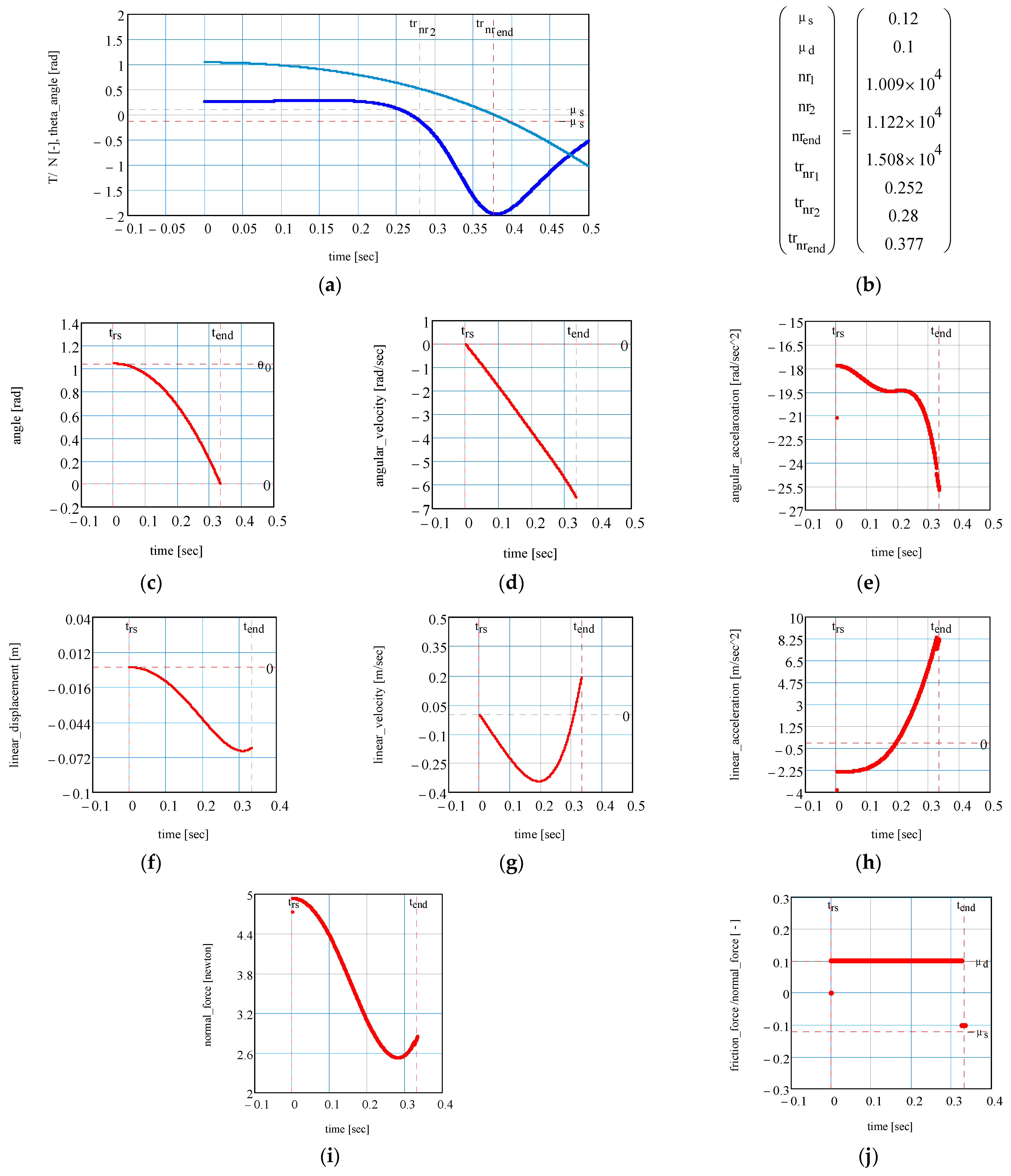
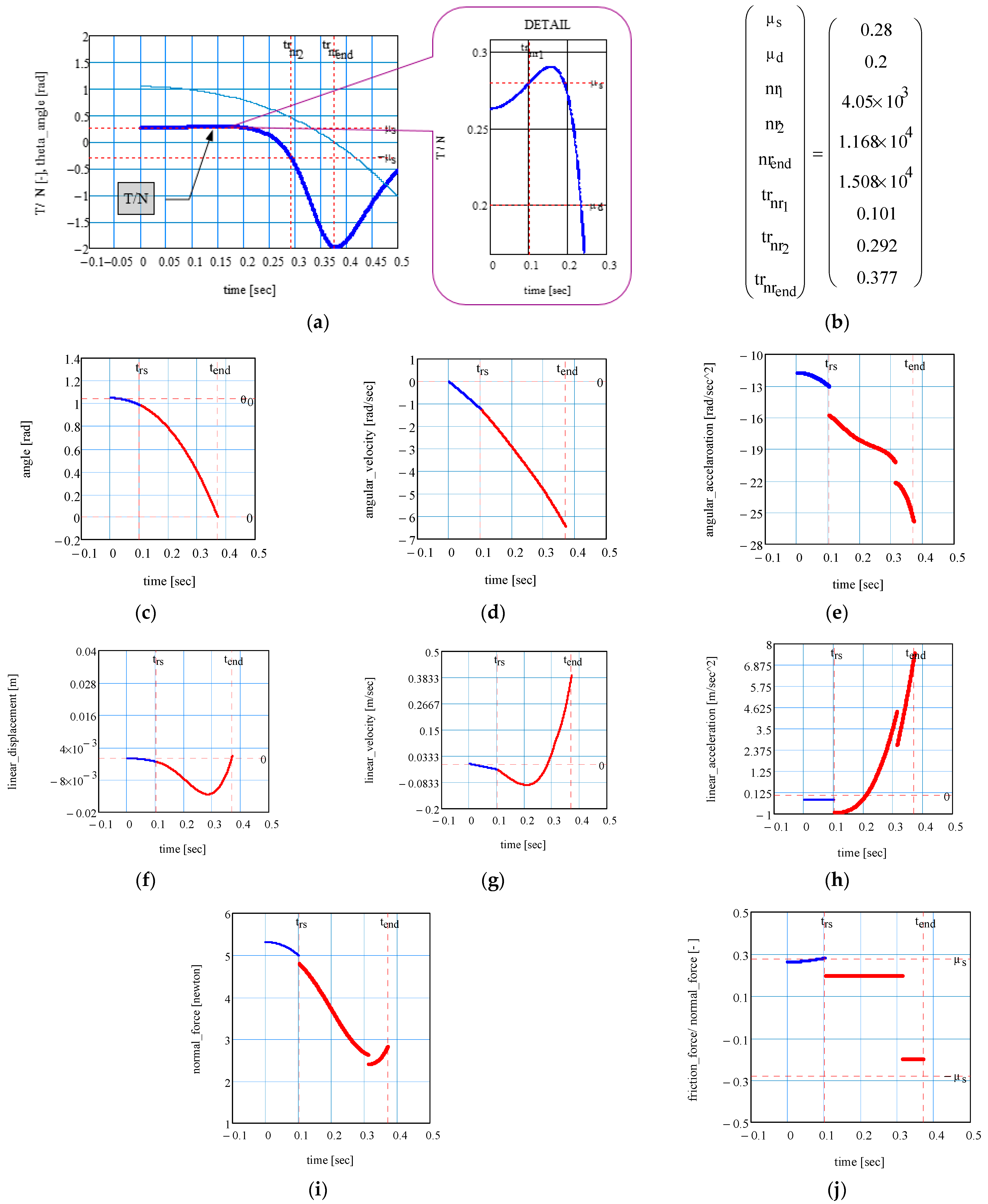
3.2. Validation of Analytical Results

The dynamical simulation software MSC.ADAMS 2013.2 was used for corroborating the theoretical results from the previous section. First, the body was modelled as two balls with the rigidly attached cylindrical rod, as presented in Figure 17a. The software enables the determination of the model’s inertial characteristics, as presented in Figure 17b. One of the balls is in contact with a horizontal metallic plate; then, the body is rotated about a horizontal axis passing through the centre of the ball until the angle between the axis of the body and the horizontal axis becomes ${\theta }_o$. Two ball–plate contacts are defined: the first contact between the ball and the horizontal plate is necessary to define the tribological parameters of the sphere–plane pair; the second contact is required to visualise the instant when the axis of the body takes a horizontal position. When the axis of the body is horizontal, a collision between the upper ball and the plate takes place, and this moment is simply identified by the discontinuity occurring in the evolution of the kinematic parameters of first order. The variation in time of the tilt angle $\theta$, the angular velocity $\dot{\theta }$, the abscissa $x_O$ of the centre of the ball, and the linear velocity ${\dot{x}}_O$ is presented in Figure 18, Figure 19, Figure 20 and Figure 21, respectively, for comparison with the theoretical results obtained previously. Each figure presents the variation in a kinematic parameter for three distinct tribological situations; the legends of colours from the plots correlate the correspondences with the characteristic tribological parameters. The friction force was modelled as shown in Figure 4, using the coefficients ${\mu }_s \mathrm{a}\mathrm{n}\mathrm{d} {\mu }_d$. The simulation from MSC.ADAMS was made using a dry friction contact. The software requires the values of certain parameters: friction coefficients, damping coefficients, and transition velocities from sliding and stiction regimes. We considered that the viscous damping was cancelled and the transition velocities were very small ($\to 0)$, because there are no accepted zero values. If we attempt to use a more complex friction model, as in Figure 6b, we require the values of the stiction transition and friction transition velocities. Giesbers [23] shows that the evolution of the system is strongly affected by these two velocities.

It can be noted that the rotation of the rod is less affected by changes in tribological parameters, exhibiting a continuous clockwise rotation. In contrast, the motion of the centre of the lower ball is significantly influenced by the coefficients of friction. Comparing the model’s results with the theoretical findings, an excellent concordance is observed, thereby validating the theoretical model. Here, we can mention the complex motion of the centre of the lower ball as a function of the values of the coefficients of friction. For small values of the friction coefficient, the entire motion of the system is characterised by sliding. Initially, the point of contact between the ball and plane moves to the left, and then to the right. With higher friction values, pure rolling initially occurs at the point of contact, causing the centre of the lower ball to move rightward. Subsequently, while sliding begins, the movement to the right continues. Thus, the overall motion of the centre of the lower ball is a translation in a single direction.

The proposed system was analysed for launching from rest. It was observed that, based on the coefficient of static friction value, either rolling or sliding phenomena occur. With higher friction coefficient values, the motion initiates with pure rolling, which is eventually replaced by sliding. The ratio between the durations of rolling and sliding intervals changes as the coefficient of friction decreases, with the sliding intervals correspondingly increasing in length.

An emerging conclusion is that the motion of the system is enclosed between two limit situations: sliding motion and pure rolling motion. Based on this observation, it was deemed appropriate to compare the variations in kinematic parameters corresponding to these limit cases: sliding and pure rolling. The equations of motion were integrated for launching from rest, for two cases in the entire time interval: only sliding or only pure rolling occurs. Three values of the coefficient of friction were considered (Figure 22, Figure 23 and Figure 24) and the variation in kinematic parameters was compared. One can notice the following:

-

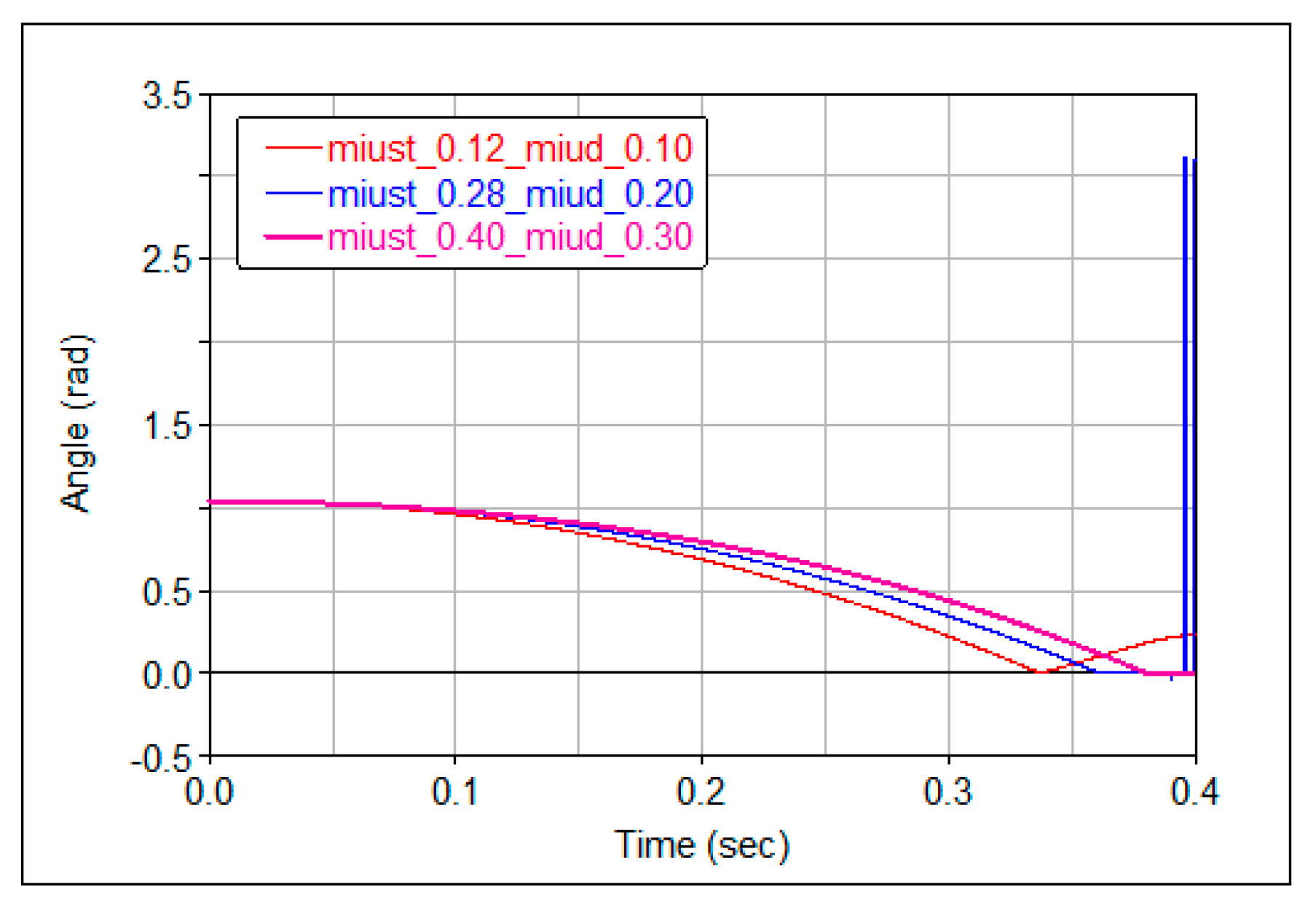
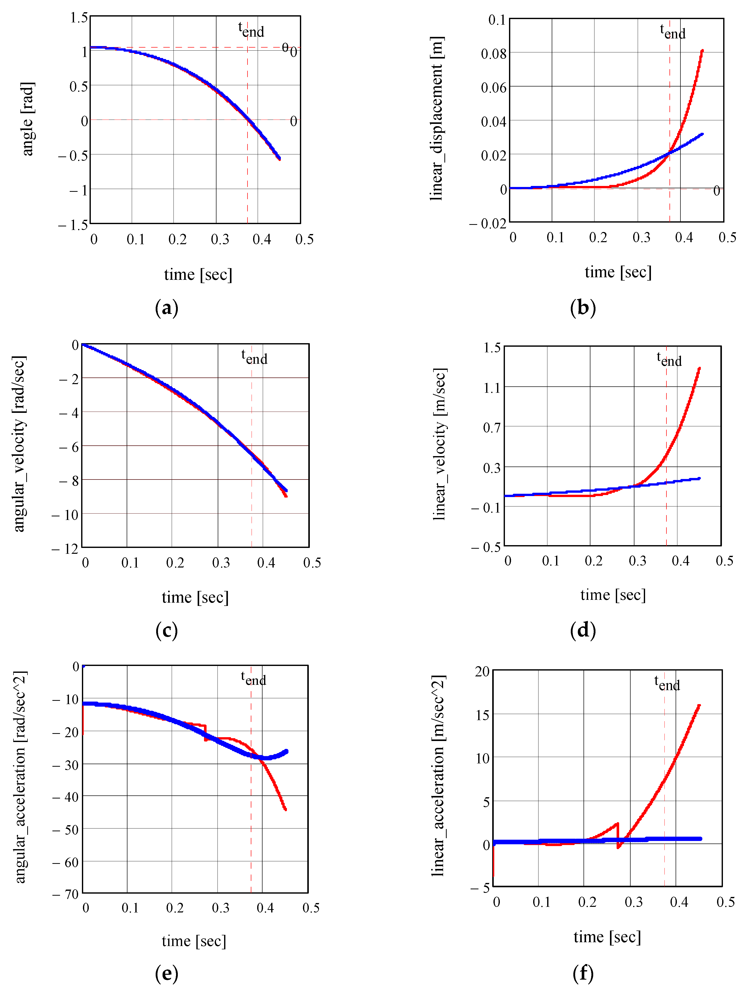
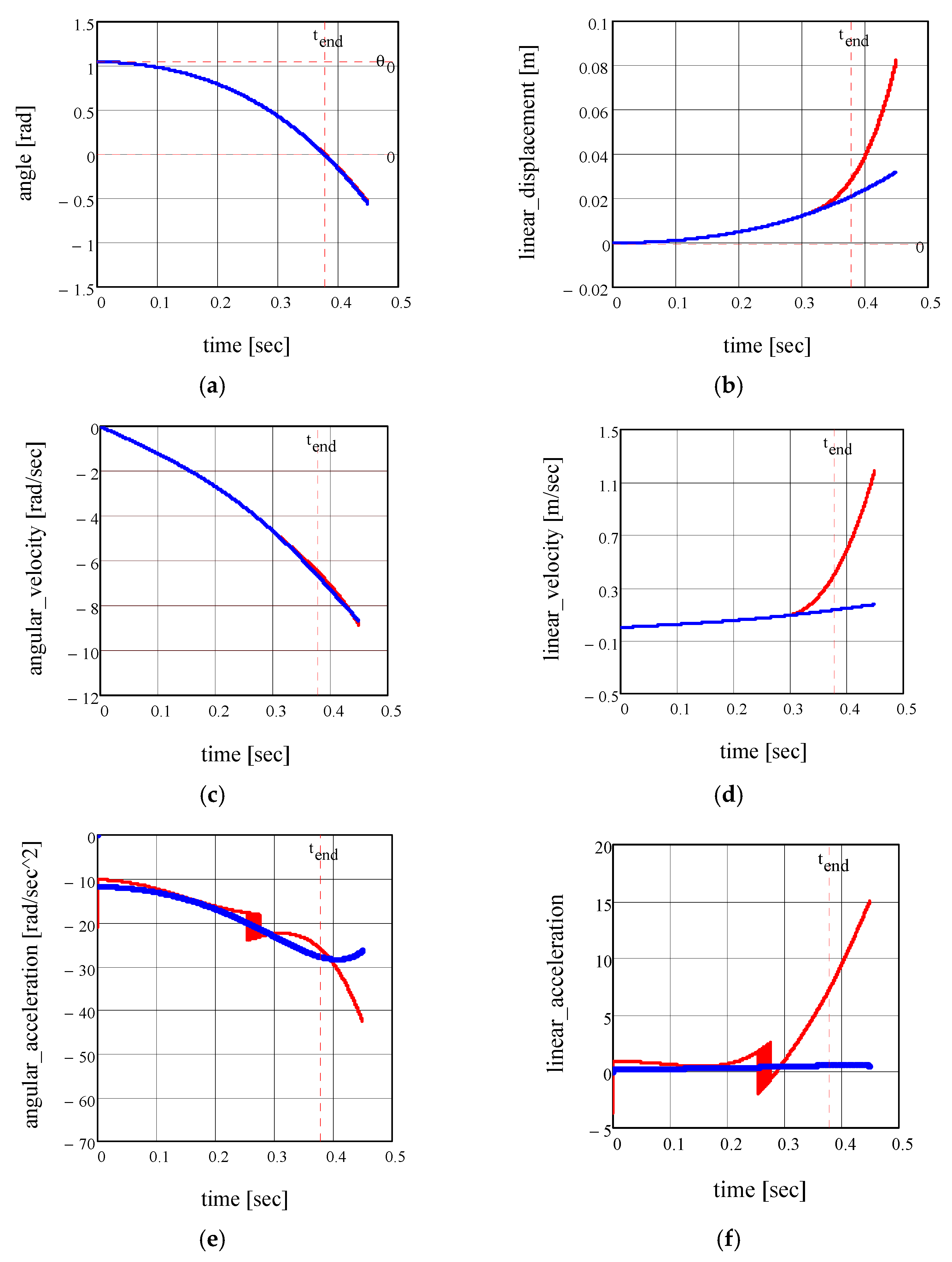
For the tilt angle of the axis of the system, the variations corresponding to the two limit cases are similar;

-

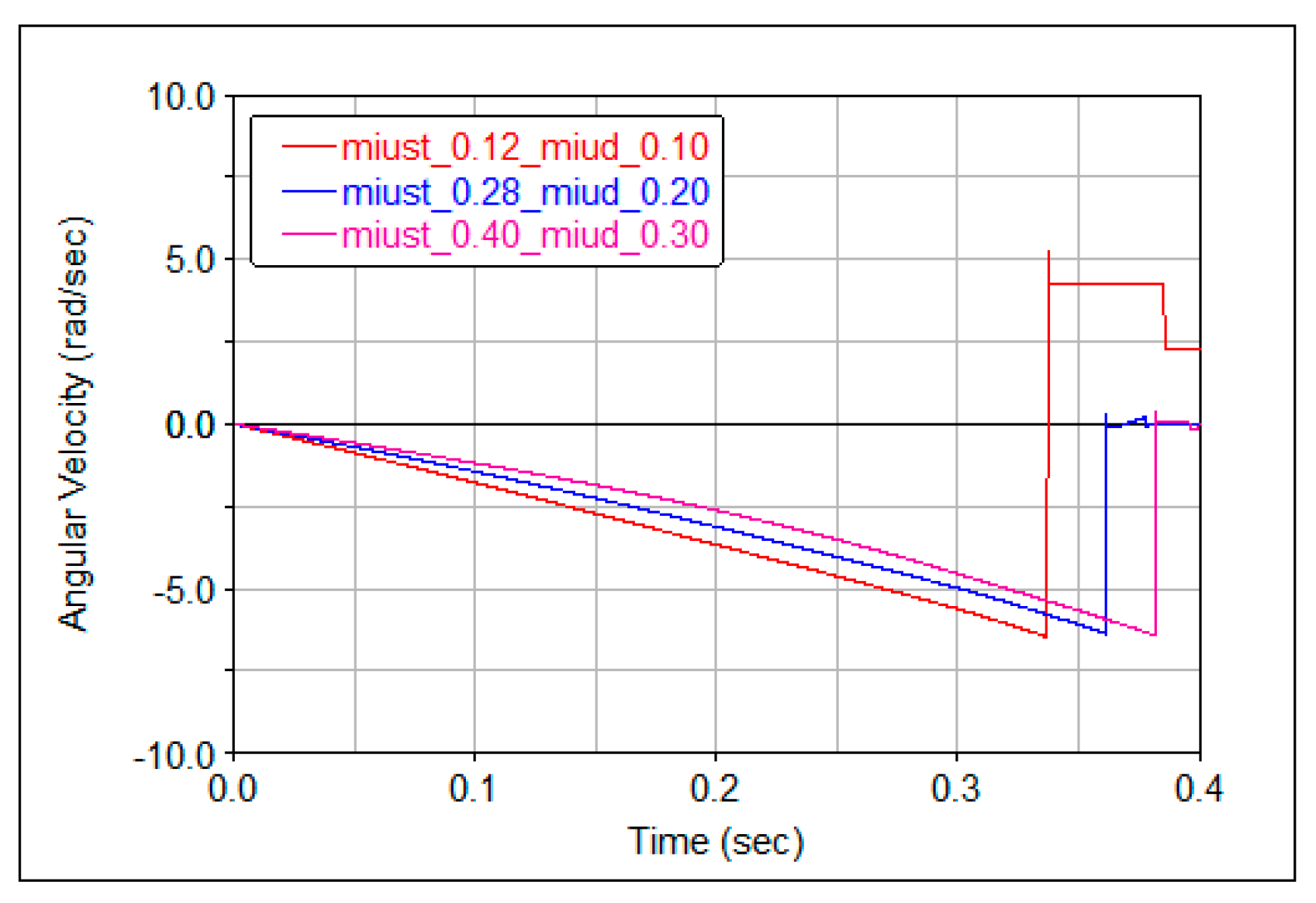
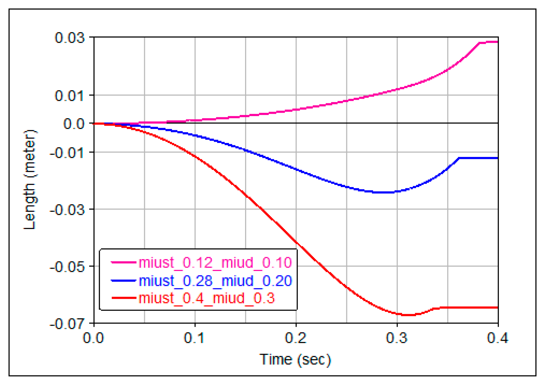
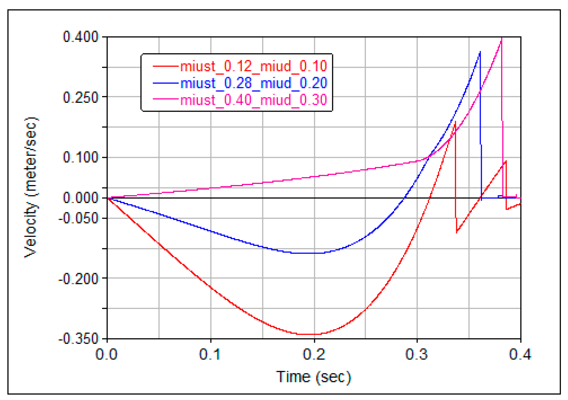
For the motion of the centre of the lower ball, the plots for rolling and sliding are completely different.

When the coefficient of friction increases up to a critical value, the effect of discontinuity occurs (Figure 25).

From the above, it can be concluded that a simplified model that considers only one type of motion (either sliding or rolling) is not applicable.

It can be observed that as the coefficient of dynamic friction increases, the likelihood of encountering discontinuities in the second-order kinematic parameters also increases. Marques [4] attributes this effect to the strong discontinuities introduced by both the Coulomb friction model and the Stribeck friction model. These models lead to “high numerical instability during the initial phase due to their discontinuity for zero velocity” [4]. Additionally, it should be noted that it is not possible to simulate the mechanism motion with the two friction models using a variable time step algorithm, since the algorithm is not able to proceed when it deals with the discontinuous behaviour [4]. Concerning the discontinuities of the accelerations of the system, presented in Figure 25, two observations must be made:

First: these discontinuities only appear on the plots for sliding motion when values exceed a certain threshold. This suggests that as the coefficient of friction increases, the probability of sliding motion decreases while the probability of pure rolling motion increases.

Second: the value of the coefficient of friction ($\mu =0.26$) from which the discontinuity phenomenon manifests is very close to the maximum value of the ratio $T/N$ corresponding to pure rolling motion ($\mathit{max}(T/N)=0.29)$. It was shown that this maximum value is decisive, during the beginning of the motion, in the transition from pure rolling to sliding motion.

4. Conclusions

The current study examines a simple dynamic system, specifically a rod that is initially at rest, with one end in contact with a horizontal plane. Dry friction forces are evident at the contact point. The dynamics simulation obtained with dedicated software showed that the magnitude of friction plays a major part in the evolution of the system; that is, for small values of velocity, the velocity of the contact point presents a shift in sign, while for greater values, the velocity has a single direction.

This paper proposes a theoretical model of the mentioned system, with an alteration of important practical significance. This modification involves attaching a ball to the end of the rod to highlight the effects of rolling friction and/or sliding friction.

It is to be remarked that the dynamics analysis software models the coefficient of friction as a continuous function of relative velocity, and, as an important consequence, the friction force cancels when the relative velocity is zero. To surpass this aspect, a friction model with discontinuity at the origin was the option because this model accepts that, when the relative velocity is zero, the friction force may take any value within an interval stipulated by the coefficient of static friction.

The problem can be solved after adopting one of the two cases of friction:

-

Firstly, rolling friction—a relationship exists between the two positional parameters, and the system has in fact only one degree of freedom; the normal and the friction force are independent.

-

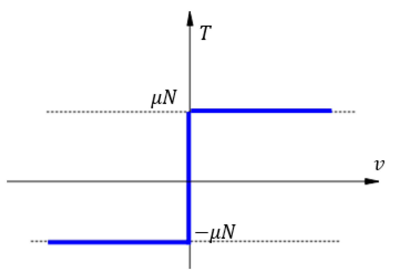
Secondly, sliding friction—when the system has two degrees of freedom but there is a relation between the normal force and the friction force stipulated by the Coulomb law.

For both cases, the nonlinear differential equations of motion are derived, along with expressions for the magnitude of the normal reaction N and the friction force T. Under the given initial conditions (launching from rest), the kinematic condition of pure rolling is met. It is accepted that, initially, the system exhibits pure rolling, which continues until the moment the dynamic condition for pure rolling |T/N| ≤ μ_st is no longer satisfied. It is concluded that there are three possible scenarios regarding the evolution of the system; one where only sliding friction is present, and the other two where rolling friction initially exists but is eventually replaced by sliding friction. The variation with time of the normal force N and the friction force T was considered useful, as well as the variation in the ratio T/N, which is a decisive parameter in defining the sliding or rolling regime. For all mentioned cases, the moments when the transition from rolling to sliding friction occurs were obtained numerically, as well as the final stage, when the body takes a horizontal position.

In order to validate the theoretical model, dynamic simulation software was used. The plotted results show the time variations of the position parameters and velocities for three sets of values for the coefficients of friction. The excellent agreement between the theoretical results and the results obtained by numerical simulation attests the correctness of the proposed analytical solution.

We consider that the main novelty of this paper consists of obtaining the plot of the variation with time of the ratio T/N and the discussions, sustained by plots, on the possibilities of evolution (pure rolling/sliding) of the system depending on the values of the coefficients of friction.

As a future work project, the authors aim to design and build an experimental device for the study of the motion of the proposed model, in order to validate the theoretical results.

References

1. Kasdin, N.J.; Paley, D.A. Engineering Dynamics: A Comprehensive Introduction; Princeton University Press: Princeton, NJ, USA, 2011; pp. 11–38. [Google Scholar]
2. Mangeron, D.; Irimiciuc, N. Mecanica Rigidelor cu Aplicaţii în Inginerie; Editura Tehnică: Bucureşti, Romania, 1978; Volume I, pp. 304–319. (In Romanian) [Google Scholar]
3. Anh, L.X. Dynamics of Mechanical Systems with Coulomb Friction; Springer: Berlin/Heidelberg, Germany, 2012; pp. 11–36. [Google Scholar]
4. Marques, F.; Flores, P.; Claro, J.C.P.; Lankarani, H.M. Modeling and analysis of friction including rolling effects in multibody dynamics: A review. Multibody Syst. Dyn. 2019, 45, 223–244. [Google Scholar] [CrossRef]
5. Threlfall, D.C. The inclusion of Coulomb friction in mechanisms programs with particular reference to DRAM au programme DRAM. Mech. Mach. Theory 1978, 13, 475–483. [Google Scholar] [CrossRef]
6. Ambrósio, J.A.C. Impact of rigid and flexible multibody systems: Deformation description and contact model. Virtual Nonlinear Multibody Syst. 2003, 103, 57–81. [Google Scholar]
7. Andersson, S.; Söderberg, A.; Björklund, S. Friction models for sliding dry, boundary and mixed lubricated contacts. Tribol. Int. 2007, 40, 580–587. [Google Scholar] [CrossRef]
8. Drincic, B. Mechanical Models of Friction That Exhibit Hysteresis, Stick-Slip, and the Stribeck Effect. Ph.D. Thesis, University Michigan, Ann Arbor, MI, USA, 2012; pp. 84–99. Available online: https://deepblue.lib.umich.edu/bitstream/handle/2027.42/93899/bojanad_1.pdf?sequence=1&isAllowed=y (accessed on 21 March 2024).
9. Bowden, F.P.; Leben, L. The nature of sliding and the analysis of friction. Proc. R. Soc. Lond. Ser. A Math. Phys. Sci. 1939, 169, 371–391. [Google Scholar] [CrossRef]
10. Johannes, V.I.; Green, M.A.; Brockley, C.A. The role of the rate of application determining the static friction coefficient. Wear 1973, 24, 381–385. [Google Scholar] [CrossRef]
11. Dahl, P.R. A Solid Friction Model. Technical Report; The Aerospace Corporation: El Segundo, CA, USA, 1968; pp. 12–17. [Google Scholar]
12. Dahl, P.R. Solid friction damping in mechanical vibrations. AIAA J. 1976, 14, 1675–1682. [Google Scholar] [CrossRef]
13. Canudas de Wit, C.; Olsson, H.; Åström, K.J.; Lischinsky, P. A new model for control of systems with friction. IEEE Trans. Autom. Control 1995, 40, 419–425. [Google Scholar] [CrossRef]
14. Rill, G.; Schuderer, M. A Second-Order Dynamic Friction Model Compared to Commercial Stick–Slip Models. Modelling 2023, 4, 366–381. [Google Scholar] [CrossRef]
15. Wang, H.; Cui, J.; Wu, J.; Tan, J. Dynamic Friction-Slip Model Based on Contact Theory. Machines 2022, 10, 951. [Google Scholar] [CrossRef]
16. Tustin, A. The effects of backlash and of speed-dependent friction on the stability of closed-cycle control systems. J. Inst. Electr. Eng. Part I Gen. 1947, 94, 143–151. [Google Scholar] [CrossRef]
17. Bo, L.C.; Pavelescu, D. the fiction-speed relation and its influence on the critical velocity of the stick-slip motion. Wear 1982, 82, 277–289. [Google Scholar]
18. Armstrong-Helouvry, B. Control of Machines with Friction; Kluwer Academic Publishers: Boston, MA, USA, 1991; pp. 63–93. [Google Scholar]
19. Parovik, R.; Shakirova, A.; Firstov, P. Mathematical model of the stick-slip effect for describing the “drum-beat” seismic regime during the eruption of the Kizimen volcano in Kamchatka. AIP Conf. Proc. 2022, 2467, 080015. [Google Scholar] [CrossRef]
20. Shakirova, A.A.; Firstov, P.P.; Parovik, R.I. Phenomenological model of the generation of the seismic mode drumbeats earthquakes accompanying the eruption of Kizimen volcano in 2011–2012. Vestn. KRAUNC. Fiz.-Mat. Nauki. 2020, 33, 86–101. [Google Scholar] [CrossRef]
21. Pennestrì, E.; Valentini, P.P.; Vita, L. Multibody dynamics simulation of planar linkages with Dahl friction. Multibody Syst. Dyn. 2007, 17, 321–347. [Google Scholar] [CrossRef]
22. Pop, N.; Ungureanu, M.; Pop, A.I. An Approximation of Solutions for the Problem with Quasistatic Contact in the Case of Dry Friction. Mathematics 2021, 9, 904. [Google Scholar] [CrossRef]
23. Giesbers, J. Contact Mechanics in MSC Adams—A technical evaluation of the contact models in multibody dynamics software MSC Adams. Bachelor’s Thesis, University Twente, Enschede, Holland, 2012; pp. 13–19. [Google Scholar]
Figure 1. The relative motion and the components of the torsor of reactions at a point-concentrated contact.
Axioms 13 00372 g001
Figure 2. Coulomb friction model of dry friction force.
Axioms 13 00372 g002
Figure 3. Continuous model approximations for Coulomb friction: (a) linear model; (b) polynomial approximation; (c) discontinuous ramp model.
Axioms 13 00372 g003
Figure 4. The dry friction force T and its components: static friction force ( μ s t N ) and dynamic friction force μ d N .
Axioms 13 00372 g004
Figure 5. Stribeck curves: models of friction versus velocity: (a) general case; (b) particular case.
Axioms 13 00372 g005
Figure 6. Approximations of Stribeck curves: (a) linear model; (b) exponential model.
Axioms 13 00372 g006
Figure 7. The Dahl bristle friction model.
Axioms 13 00372 g007
Figure 8. The proposed dynamic system.
Axioms 13 00372 g008
Figure 9. The general form of the dependency T / N .
Axioms 13 00372 g009
Figure 10. For small friction values, sliding motion manifests in the entire interval T ( 0 ) / N ( 0 ) > μ s , max ( T / N ) > μ s .
Axioms 13 00372 g010
Figure 11. For medium friction values, pure rolling initially exists in the interval [ 0 , t r 1 ] , followed by sliding motion T ( 0 ) / N ( 0 ) μ s , max ( T / N ) > μ s .
Axioms 13 00372 g011
Figure 12. For substantial friction forces, in the domain [ 0 , t r 2 ] , pure rolling manifests, and after that, sliding motion occurs T ( 0 ) / N ( 0 ) μ s , max ( T / N ) μ s .
Axioms 13 00372 g012
Figure 13. The body modelled for applying the deduced relations.
Axioms 13 00372 g013
Figure 14. For the values μ s = 0.12 and μ d = 0.10 , the variation with time of (a) the ratio between the friction force and normal reaction, T / N , for pure rolling; (b) tribological parameters and characteristic times; (c) the position angle θ ; (d) the angular velocity θ ˙ ; (e) the angular acceleration θ ¨ ; (f) the position of the centre of the ball x O ; (g) the velocity of the centre of the ball x ˙ O ; (h) the acceleration of the centre of the ball x ¨ O ; (i) the normal reaction N ; (j) the actual ratio between the friction force and normal reaction T / N . The red colour corresponds to the sliding regime and the blue colour corresponds to the rolling regime.
Axioms 13 00372 g014
Figure 15. For the values μ s = 0.28 and μ d = 0.20 , the variation with time of (a) the ratio between the friction force and normal reaction, T / N , for pure rolling; (b) tribological parameters and characteristic times; (c) the position angle θ ; (d) the angular velocity θ ˙ ; (e) the angular acceleration θ ¨ ; (f) the position of the centre of the ball x O ; (g) the velocity of the centre of the ball x ˙ O ; (h) the acceleration of the centre of the ball x ¨ O ; (i) the normal reaction N ; (j) the actual ratio between the friction force and normal reaction T / N . The red colour corresponds to sliding regime and the blue colour corresponds to the rolling regime.
Axioms 13 00372 g015
Figure 16. For the values μ s = 0.40 and μ d = 0.30 , the variation with time of (a) the ratio between the friction force and normal reaction, T / N , for pure rolling; (b) tribological parameters and characteristic times; (c) the position angle θ ; (d) the angular velocity θ ˙ ; (e) the angular acceleration θ ¨ ; (f) the position of the centre of the ball x O ; (g) the velocity of the centre of the ball x ˙ O ; (h) the acceleration of the centre of the ball x ¨ O ; (i) the normal reaction N ; (j) the actual ratio between the friction force and normal reaction T / N . The red colour corresponds to sliding regime and the blue colour corresponds to the rolling regime.
Axioms 13 00372 g016
Figure 17. (a) The dynamic system modelled using MSC: ADAMS simulation software, and (b) values of inertial characteristics.
Axioms 13 00372 g017
Figure 18. Variation in the angle of the axis of the body for the three sets of coefficients of friction.
Axioms 13 00372 g018
Figure 19. The simulated angular velocity of the body: variation for the three sets of coefficients of friction.
Axioms 13 00372 g019
Figure 20. The variation in the abscissa of the centre of the lower ball for the three sets of coefficients of friction.
Axioms 13 00372 g020
Figure 21. The variation in the velocity of the centre of the lower ball for the three sets of coefficients of friction.
Axioms 13 00372 g021
Figure 22. Comparison between results of pure rolling (blue line) and sliding (red line) hypothesis for μ d = 0.10 : (a) angular displacement θ , (b) linear displacement x O , (c) angular velocity θ ˙ , (d) linear velocity x ˙ O , (e) angular acceleration θ ¨ , (f) x ¨ O linear acceleration.
Axioms 13 00372 g022
Figure 23. Comparison between results of pure rolling (blue line) and sliding (red line) hypothesis for μ d = 0.257 : (a) angular displacement θ ; (b) linear displacement x O ; (c) angular velocity θ ˙ ; (d) linear velocity x ˙ O ; (e) angular acceleration θ ¨ ; (f)   x ¨ O linear acceleration.
Axioms 13 00372 g023
Figure 24. Comparison between results for pure rolling (blue line) and sliding (red line) hypothesis for μ d = 0.3 : (a) angular displacement θ ; (b) linear displacement x O ; (c) angular velocity θ ˙ ; (d) linear velocity x ˙ O ; (e) angular acceleration θ ¨ ; (f) linear acceleration x ¨ O .
Axioms 13 00372 g024
Figure 25. The effect of the coefficient of friction discontinuities on the evolution of angular velocity of the body: (a) μ = 0.25 ; (b) detail μ = 0.25 ; (c) μ = 0.26 ; (d) detail μ = 0.26 ; (e) μ = 0.3 ; (f) detail μ = 0.3 . The pure rolling case is represented with blue line and sliding case with red line.
Axioms 13 00372 g025
Disclaimer/Publisher’s Note: The statements, opinions and data contained in all publications are solely those of the individual author(s) and contributor(s) and not of MDPI and/or the editor(s). MDPI and/or the editor(s) disclaim responsibility for any injury to people or property resulting from any ideas, methods, instructions or products referred to in the content.